Article

Optimal Combination of the Splitting–Linearizing Method to SSOR and SAOR for Solving the System of Nonlinear Equations

1
Center of Excellence for Ocean Engineering, National Taiwan Ocean University, Keelung 202301, Taiwan
2
Department of Mathematics, College of Sciences and Humanities in Al-Kharj, Prince Sattam bin Abdulaziz University, Alkharj 11942, Saudi Arabia
3
Department of Basic Engineering Science, Faculty of Engineering, Menofia University, Shebin El-Kom 32511, Egypt
4
Department of Mechanical Engineering, National United University, Miaoli 36063, Taiwan
*
Author to whom correspondence should be addressed.
Mathematics 2024, 12(12), 1808; https://doi.org/10.3390/math12121808
Submission received: 12 May 2024 / Revised: 1 June 2024 / Accepted: 5 June 2024 / Published: 11 June 2024

Abstract

The symmetric successive overrelaxation (SSOR) and symmetric accelerated overrelaxation (SAOR) are conventional iterative methods for solving linear equations. In this paper, novel approaches are presented by combining a splitting–linearizing method with SSOR and SAOR for solving a system of nonlinear equations. The nonlinear terms are decomposed at two sides through a splitting parameter, which are linearized around the values at the previous step, obtaining a linear equation system at each iteration step. The optimal values of parameters are determined to minimize the reciprocal of the maximal projection, which are sought in preferred ranges using the golden section search algorithm. Numerical tests assess the performance of the developed methods, namely, the optimal splitting symmetric successive over-relaxation (OSSSOR), and the optimal splitting symmetric accelerated over-relaxation (OSSAOR). The chief advantages of the proposed methods are that they do not need to compute the inverse matrix at each iteration step, and the computed orders of convergence by OSSSOR and OSSAOR are between 1.5 and 5.61; they, without needing the inner iterations loop, converge very fast with saving CPU time to find the true solution with a high accuracy.

1. Introduction

The paper is focused on novel iterative methods for solving
F ( x ) = 0 , x : = ( x 1 , , x n ) T R n , F : = ( F 1 , , F n ) T R n .
Nonlinear equations are ubiquitous as the main mathematical models for depicting physical phenomena. Many nonlinear ordinary differential equations and partial differential equations after discretizations become finite dimensional systems of nonlinear equations. In practice, some decomposition techniques in linear algebra such as the Cholesky decomposition L L T , L U decomposition as well as the Q R decomposition of a given matrix, can also be viewed as nonlinear equations for finding L , U , Q and R . In the L U decomposition of a matrix A = L U , L is a lower triangular matrix, and U is an upper triangular matrix. In the Q R decomposition of a matrix A = Q R , Q is an orthonormal matrix, and R is an upper triangular matrix.
In the study of evolutionary type algorithm for solving nonlinear equations, Liu [1] has constructed an invariant manifold by
h ( x , t ) = Q ( t ) 2 F ( x ) 2 1 2 F ( x 0 ) 2 = 0 ,
where F is the residual of Equation (1) defined in terms of the Euclidean norm; Q ( 0 ) = 1 and Q ( t ) > 0 is a monotonically increasing function of t, and x 0 is an initial guess of solution.
Let B = [ b i j ] be the Jacobian matrix of Equation (1) with b i j = F i / x j . Liu [1] found an important function to qualify the convergence behavior of an iterative scheme:
a 0 ( x ) : = F 2 E F 2 [ F · ( E F ) ] 2 1 ,
where E = B B T . When a 0 ( x ) tends to one, the solution x is obtained approximately. Liu [1] proposed a method to find a better descent direction u by minimizing
min u , v = B u a 0 ( x ) : = F 2 v 2 ( F · v ) 2 1 .
It is interesting that the Newtonian descent direction u is given by
B u = F ,
which renders v = B u = F , and hence, a 0 ( x ) = 1 in Equation (4). In the sense of the optimality of Equation (4), the Newton iteration method is the optimal one, which is convergent quadratically. However the Newton iteration method is sensitive to the initial guess of the solution and the computation of B k 1 at each iteration step is expensive. Indeed, there are many effective iteration methods by extending and modifying the Newton iteration method to solve the nonlinear Equations [2,3,4,5,6]. Recently, Al-Obaidi and Darvish [7] gave a comparative study on the qualification criteria for three categories nonlinear solvers for solving nonlinear equations. The multi-point and higher-order iterative algorithms based on the Newton technique for solving nonlinear equations can be seen in [8,9].
The methods of symmetric successive over-relaxation and symmetric accelerated over-relaxation [10,11,12,13] iteratively solve x R n from
A x = b ,
where the coefficient matrix A R n × n has nonzero diagonal elements, and b R n is given.
Let y : = A x . We attempt to find the optimal approximation of b to y by an optimization method. The orthogonal projection is regarded as the approximation to b by y , whose error vector is written as
e : = b b · y y y y .
The best approximation can be found by minimizing
min x e 2 = min x b 2 ( b · y ) 2 y 2 ,
or equivalently maximizing the square of the orthogonal projection of b to y , i.e.,
max x ( b · y ) 2 y 2 .
Due to this reason, the solution of the above equation will be named the maximal projection solution.
Since b is a given nonzero constant vector, we can recast Equation (9) to
max x ( b · y ) 2 b 2 y 2 ,
which does not influence the solution of x . The following merit function
min x f = b 2 y 2 ( b · y ) 2 1 ,
which is the reciprocal of Equation (10), has the same form to Equation (4); it is used to seek the optimal searching direction in the numerical solution of nonlinear equations.
Based on Equation (11), Liu [14] developed a double optimal iterative algorithm (DOIA) to solve the nonlinear equations by solving
B k u k = F k ,
at each iteration step to find the best descent direction u k in an affine Krylov subspace.
In the methods of symmetric successive over-relaxation (SSOR), accelerated over-relaxation (AOR) and symmetric accelerated over-relaxation (SAOR) the optimal values of the parameters are usually difficult to achieve [11,12,15]. Here, we are going to search the optimal values of the parameters used in the combination of a splitting technique to the SSOR and SAOR and optimize the related parameters by the minimization technique in Equation (11) to solve the nonlinear equations.
Basically, many algorithms, like the DOIA in [14] and the double iterations method in [16], required us to solve a linear system (12) in each iteration step to determine the precise descent vector u k in the current step. This is carried out in general through an inner iterations loop. In the proposed iterative algorithms, the SSOR and SAOR are automatically merged into the outer iterations, which do not need to carry out the loop of inner iterations at each iteration step; refer to the pseudo-code to be presented in Section 4. In doing so, a lot of computational time can be saved. Therefore, the main superiority of the new method are its low computational complexity, saving computational time and not sensitive to the initial guess of x 0 . However, a major drawback of the SSOR and SAOR is that some values of the parameters must be properly selected. We are going to overcome this difficulty in this paper, and we propose a novel linearization method which is different from the Newton iteration method; the computation of B k and its inversion B k 1 at each iteration step are no longer needed.
Other sections of the paper are arranged as follows. Section 2 briefly sketches some conventional iterative algorithms for solving linear equations, including the successive over-relaxation (SOR) method, its symmetrization as the symmetry successive over-relaxation (SSOR) method, and the symmetry accelerated over-relaxation (SAOR) method. In Section 3, a matrix–vector form of nonlinear equations is introduced, which is linearized to a step-by-step varying linear system through a splitting parameter. By applying SSOR and minimizing a merit function based on the maximal projection method, we develop an optimal splitting symmetry successive over-relaxation (OSSSOR); combining the splitting–linearizing technique with SAOR, we develop an optimal splitting symmetry accelerated over-relaxation (OSSAOR) method for solving nonlinear equations. In Section 4, a pseudo-code for OSSSOR is sketched. In Section 5, a local convergence analysis is initiated. Some examples of nonlinear equations are examined in Section 6 by OSSSOR and OSSAOR. Finally, the conclusions in Section 7 summarize and highlight the main achievements.

2. Reviews of Two Symmetric Iterative Methods for Linear Equations

In Equation (6), the coefficient matrix is decomposed to
A = D U L ,
where D , U and L are, respectively, the diagonal, strictly upper triangular and strictly lower triangular parts of A .
It follows from Equations (6) and (13) the SOR iterative method [13]:
( D w L ) x k + 1 = w b + ( 1 w ) D x k + w U x k .
For the purpose of convergence, the relaxation parameter w is constrained by 0 < w < 2 . In Equation (14), owing to the lower triangular matrix of D w L , x k + 1 is easily computed from the previous step value x k by using the forward substitution method.
On the other hand, the SSOR is [17]
( D w L ) x k + 1 / 2 = w b + ( 1 w ) D x k + w U x k ,
( D w U ) x k + 1 = w b + ( 1 w ) D x k + 1 / 2 + w L x k + 1 / 2 ,
which is convergent faster than SOR.
While the AOR is [11]
( D σ L ) x k + 1 = w b + ( 1 w ) D x k + w U x k + ( w σ ) L x k ,
a symmetric AOR (SAOR) is [12]
( D σ L ) x k + 1 / 2 = w b + ( 1 w ) D x k + w U x k + ( w σ ) L x k , ( D σ U ) x k + 1 = w b + ( 1 w ) D x k + 1 / 2 + w L x k + 1 / 2 + ( w σ ) U x k + 1 / 2 .

3. Nonlinear Equations

Recently, Liu et al. [18] applied the dynamical optimal techniques in the SSOR, AOR, and SAOR for solving linear equations. We extend these results to the system of nonlinear equations in Equation (1), which can be recast to a matrix–vector form:
A ˜ x + B ( x ) x = b ˜ ,
where A ˜ R n × n is a constant matrix, B R n × n is a matrix function of x , and b ˜ R n is a constant vector.
To Equation (19), we add a splitting parameter s:
A ˜ x + s B ( x ) x = b ˜ + ( s 1 ) B ( x ) x ,
which can be linearized around x k by
A ˜ x + s B ( x k ) x = b ˜ + ( s 1 ) B ( x k ) x k .
Upon letting
A ( s ) : = A ˜ + s B ( x k ) , b ( s ) : = b ˜ + ( s 1 ) B ( x k ) x k ,
we can derive a step-by-step varying linear system:
A ( s ) x = b ( s ) ,
where both A and b are functions of s and x k . However, for saving notations, the dependence on x k is not written out explicitly.

3.1. Optimal Splitting Symmetric Successive Over-Relaxation Method

According to the SSOR in Section 2, we can derive an iterative scheme for Equation (23):
[ D ( s ) w L ( s ) ] x k + 1 / 2 = w b ( s ) + ( 1 w ) D ( s ) x k + w U ( s ) x k ,
[ D ( s ) w U ( s ) ] x k + 1 = w b ( s ) + ( 1 w ) D ( s ) x k + 1 / 2 + w L ( s ) x k + 1 / 2 .
Now, D , U and L are also functions of s and x k , such that it is a nonlinear iterative scheme. Equations (24) and (25) involve two parameters ( s , w ) to be determined as follows. Let
H 1 = [ D ( s ) w U ( s ) ] x k + 1 / 2 , H 2 = w b ( s ) + ( 1 w ) D ( s ) x k + 1 / 2 + w L ( s ) x k + 1 / 2 ,
where x k + 1 / 2 is calculated from Equation (24). Insert them into Equation (11), we can seek the optimal values of ( s k , w k ) by minimizing
min ( s k , w k ) ( a , b ) × ( c , d ) f k + 1 / 2 = H 1 2 H 2 2 ( H 1 · H 2 ) 2 .
The algorithm in Equations (24), (25) and (27) is a new iterative scheme for solving nonlinear equations system (1), which is shortened as an optimal splitting symmetric successive over-relaxation (OSSSOR) method. A two-dimensional golden section search algorithm as listed in the Appendix A is applied for determining ( s k , w k ) in Equation (27), of which only a few steps are spent at each iteration, when a loose convergence criterion is taken.

3.2. Optimal Splitting Symmetric Accelerated Over-Relaxation Method

In general, the symmetric accelerated over-relaxation method (SAOR) is convergent faster than the symmetric successive over-relaxation method (SSOR) for solving linear equations. According to the SAOR in Section 2, we can derive a nonlinear iterative scheme for Equation (23):
[ D ( s ) σ L ( s ) ] x k + 1 / 2 = w b ( s ) + ( 1 w ) D ( s ) x k + w U ( s ) x k + ( w σ ) L ( s ) x k ,
[ D ( s ) σ U ( s ) ] x k + 1 = w b ( s ) + ( 1 w ) D ( s ) x k + 1 / 2 + w L ( s ) x k + 1 / 2 + ( w σ ) U ( s ) x k + 1 / 2 .
Equations (28) and (29) involve three parameters ( s , w , σ ) to be determined as follows. Let
R 1 = [ D ( s ) σ U ( s ) ] x k + 1 / 2 , R 2 = w b ( s ) + ( 1 w ) D ( s ) x k + 1 / 2 + w L ( s ) x k + 1 / 2 + ( w σ ) U ( s ) x k + 1 / 2 ,
where x k + 1 / 2 is calculated from Equation (28). Insert them into Equation (11), obtaining
min ( s k , w k , σ k ) ( A , B ) × ( a , b ) × ( c , d ) R 1 2 R 2 2 ( R 1 · R 2 ) 2 ;
it is used to determine ( s k , w k , σ k ) . However, this minimization in three dimensions would spend much time. We take a simpler one by
min s k [ A , B ] min ( w k , σ k ) ( a , b ) × ( c , d ) R 1 2 R 2 2 ( R 1 · R 2 ) 2 ,
where we let s k run in a few points in ( A , B ) by s k j = A + ( j 1 ) ( B A ) / ( N s 1 ) , j = 1 , , N s with N s = 6 . The minimization in the second part is carried out by the golden section search algorithm.
The algorithm in Equations (28), (29) and (32) is a new iterative scheme for solving nonlinear equations system (1), which is shortened as an optimal splitting symmetric accelerated over-relaxation (OSSAOR) method.

4. Numerical Algorithm

In this section, we take OSSSOR as an example to write its pseudo-code, where the two-dimensional golden section algorithm is listed in the Appendix A. Before that, we need two codes to solve Equations (24) and (25) forward and backward, respectively. In the code, n is the dimension of the nonlinear equations, b(I) is the I-component of b , and A(I,J) is the IJ-component of A ; A and b are inputs, and c is the output (Algorithms 1–3).
Algorithm 1: FSOL  (n,A,b,c)
Give n, A and b
DO I = 1,n
SUM = 0
DO J = 1, I − 1
SUM = SUM + A(I,J) × c(J)
Enddo of J
c(I) = (b(I) − SUM)/A(I,I)
Enddo of I
Algorithm 2: BSOL (n,A,b,c)
Give n, A and b
DO K = 1,n
I = n − K+1
SUM = 0
DO J = I + 1,n
SUM = SUM + A(I,J)×c(J)
Enddo of J
c(I) = (b(I) − SUM)/A(I,I)
Enddo of K
Algorithm 3: OSSSOR
1: Give n, F , initial value x 0 , and ε
2: Give a, b, c and d
3: Do k = 0 , 1 ,
4: Call GOLDEN(a, b, c, d, f k + 1 / 2 , s k , w k )
5: Compute A k ( s k ) = A ˜ + s k B ( x k )
6: Compute b o ( s k ) = b ˜ + ( s k 1 ) B ( x k ) x k
7: Compute D k ( s k ) , L k ( s k ) and U k ( s k )
8: Compute A k ( s k ) = D k ( s k ) w k L k ( s k )
9: Compute b k ( s k ) = w k b o ( s k ) + ( 1 w k ) D k ( s k ) x k + w k U k ( s k ) x k
10: Call FSOL(n, A k ( s k ) , b k ( s k ) , x k + 1 / 2 )
11: Compute A k ( s k ) = D k ( s k ) w k U k ( s k )
12: Compute b k ( s k ) = w k b o ( s k ) + ( 1 w k ) D k ( s k ) x k + 1 / 2 + w k L k ( s k ) x k + 1 / 2
13: Call BSOL(n, A k ( s k ) , b k ( s k ) , x k + 1 )
14: If F ( x k + 1 ) < ε , stop
15: Otherwise, go to 3
We notice that b o denotes b ( s ) in Equation (22); f k + 1 / 2 in Equation (27) is the input of GOLDEN, whose outputs are s k and w k ; the output of FSOL is x k + 1 / 2 ; and the output of BSOL is x k + 1 .

5. Local Convergence

We suppose that at the kth iteration the nonlinear equations are linearized to
A ( k ) x = b ( k ) ,
where
A ( k ) = D ( k ) U ( k ) L ( k ) .
We first discuss the SOR:
( D ( k ) w L ( k ) ) x k + 1 = w b ( k ) + ( 1 w ) D ( k ) x k + w U ( k ) x k .
Theorem 1.
A new iterative form of SOR in Equation (35) is
x k + 1 = x k + u k ,
where u k is the kth step descent vector, obtained from a forward solution of
( D ( k ) w L ( k ) ) u k = w r k ;
r k = b ( k ) A ( k ) x k
is the kth step residual vector.
Proof. 
We rewrite Equation (35) to
( D ( k ) w L ( k ) ) x k + 1 = ( D ( k ) w L ( k ) ) x k + w b ( k ) + [ ( 1 w ) D ( k ) + w U ( k ) ( D ( k ) w L ( k ) ) ] x k ,
which can be rearranged to
( D ( k ) w L ( k ) ) x k + 1 = ( D ( k ) w L ( k ) ) x k + w b ( k ) w ( D ( k ) U ( k ) L ( k ) ) x k .
In view of Equations (34) and (38), we have
( D ( k ) w L ( k ) ) x k + 1 = ( D ( k ) w L ( k ) ) x k + w b ( k ) w A ( k ) x k = ( D ( k ) w L ( k ) ) x k + w r k ;
removing ( D ( k ) w L ( k ) ) x k to the left-hand side yields
( D ( k ) w L ( k ) ) ( x k + 1 x k ) = w r k .
In terms of u k in Equation (36), we can derive Equation (37). □
Motivated by the new form of the SOR in Equations (36)–(38), we can prove the following result.
Theorem 2.
For SOR, if the following condition is satisfied
A ( k ) u k 2 2 r k T A ( k ) u k < 0 ,
then the iterative algorithm is local convergence with
r k + 1 < r k .
Proof. 
In terms of residual vector, we can rewrite Equation (36) to
r k + 1 = r k A ( k ) u k .
Taking the squared norms of both sides yields
r k + 1 2 = r k 2 2 r k T A ( k ) u k + A ( k ) u k 2 .
If the condition (43) is satisfied, then
r k + 1 2 < r k 2 .
Taking the square roots of both sides, Equation (44) is proven. □
As shown in Equation (11), we choose the optimal values of the parameters s and w to minimize
min s , w f = r k 2 A ( k ) u k 2 ( r k T A ( k ) u k ) 2 1 .
If A ( k ) u k = r k is satisfied, f = 1 can be achieved. Then by means of Equation (46), we can derive
r k + 1 2 = r k 2 A ( k ) u k 2 .
It guarantees the local convergence of the proposed iterative algorithm. For the SSOR the similar results can be derived for the backward part with D ( k ) w L ( k ) in Equation (37) being replaced by D ( k ) w U ( k ) . We can conclude that
r k + 1 < r k + 1 / 2 < r k
in the SSOR. Thus, the local convergence of SSOR can be verified.
For the AOR,
( D ( k ) σ L ( k ) ) x k + 1 = w b ( k ) + ( 1 w ) D ( k ) x k + w U ( k ) x k + ( w σ ) L ( k ) x k ,
the proof of local convergence is given as follows, which involves three parameters.
Theorem 3.
A new iterative form of AOR in Equation (51) is
x k + 1 = x k + u k ,
where u k is the kth step descent vector, obtained from a forward solution of
( D ( k ) σ L ( k ) ) u k = w r k ;
r k = b ( k ) A ( k ) x k
is the kth step residual vector.
Proof. 
We rewrite Equation (51) to
( D ( k ) σ L ( k ) ) x k + 1 = ( D ( k ) σ L ( k ) ) x k + w b ( k ) + ( 1 w ) D ( k ) x k + w U ( k ) x k + ( w σ ) L ( k ) x k ( D ( k ) σ L ( k ) ) x k .
In view of Equations (34) and (54), which can be rearranged to
( D ( k ) σ L ( k ) ) x k + 1 = ( D ( k ) σ L ( k ) ) x k + w b ( k ) w A ( k ) x k = ( D ( k ) σ L ( k ) ) x k + w r k ;
removing ( D ( k ) σ L ( k ) ) x k to the left-hand side yields
( D ( k ) σ L ( k ) ) ( x k + 1 x k ) = w r k .
In terms of u k in Equation (52), we can derive Equation (53). □
Theorem 4.
For AOR, if the following condition is satisfied
A ( k ) u k 2 2 r k T A ( k ) u k < 0 ,
then the iterative algorithm is local convergence with
r k + 1 < r k .
Proof. 
The proof is same to that given in Theorem 2. □
If A ( k ) u k = r k is satisfied, f = 1 can be achieved, and the iterative algorithm is local convergence as shown in Equation (49). Numerical examples given below will show that f fast tends to 1.

6. Numerical Tests of Nonlinear Equations

In this section, we test the performance of OSSSOR and OSSAOR for solving nonlinear equations. To further asses the performance of the proposed algorithms, we compute the convergence order. For solving a scalar equation f ( x ) = 0 , if the iterative sequence { x n } converges to x * with f ( x * ) = 0 , the convergence order ζ can be estimated by
| x n + 1 x * | = β | x n x * | ζ ,
where β > 0 is a constant. Taking the operation ln on both sides yields
ln | x n + 1 x * | = ln β + ζ ln | x n x * | ,
ln | x n x * | = ln β + ζ ln | x n 1 x * | .
Subtracting Equation (61) by Equation (62), we can approximate ζ by
C O C : = ln x n + 1 x * x n x * ln x n x * x n 1 x * .
Similarly, for solving the nonlinear equations, we can generate the sequence x k , k = 1 , , k 0 , upon giving the initial value x 0 . We define
C O C : = ln x k 0 x * x k 0 1 x * ln x k 0 1 x * x k 0 2 x * ,
where x * is the exact solution and k 0 is the number of iterations.

6.1. Example 1

First, we solve [19]
F 1 ( x , y ) = x 3 3 x y 2 + a 1 ( 2 x 2 + x y ) + b 1 y 2 + c 1 x + a 2 y = 0 ,
F 2 ( x , y ) = 3 x 2 y y 3 a 1 ( 4 x y y 2 ) + b 2 x 2 + c 2 = 0 .
These equations have been solved in [14,19,20] by different methods, and they found five solutions.
Hirsch and Smale [19] derived a continuous Newton method governed by the following differential equation:
x ˙ ( t ) = B 1 ( x ) F ( x ) ,
x ( 0 ) = x 0 .
It can be seen that Equation (67) is difficult to calculate, because it includes an inverse of the Jacobian matrix.
Equations (65) and (66) can be written as
c 1 a 2 0 0 x y + x 2 + 2 a 1 x b 1 y 3 x y + a 1 x b 2 x 3 x 2 y 2 + a 1 y 4 a 1 x x y = 0 c 2 .
We take a 1 = 25 , b 1 = 1 , c 1 = 2 , a 2 = 3 , b 2 = 4 and c 2 = 5 . Hirsch and Smale [19] used the continuous Newton algorithm to calculate this problem and obtained ( x , y ) = ( 39.0207 , 38.2417 ) . Inserting it into F 1 and F 2 , we find that ( F 1 , F 2 ) = ( 0.339 , 0.117 ) , which indicates that the result obtained in [19] is not accurate.
In [21], with ( x 0 , y 0 ) = ( 0.1 , 0.1 ) and the number of iterations (NI) = 101, ( x , y ) = ( 0.134212 , 0.811128 ) and ( | F 1 | , | F 2 | ) = ( 1.141 × 10 7 , 8.913 × 10 7 ) were obtained. By using OSSSOR, we take ( a , b ) × ( c , d ) = ( 0.9 , 1.6 ) × ( 0.5 , 1.9 ) and ( x 0 , y 0 ) = ( 1 , 1 ) , and NI = 49 under ε = 10 15 as shown in Figure 1a by a solid line. In the whole paper, “Residual” in a figure means F , which abides the convergence criterion by F < ε .
Here, ( x , y ) = ( 0.163635 , 0.230529 ) is obtained by the OSSSOR, and ( | F 1 | , | F 2 | ) = ( 2.22 × 10 16 , 8.88 × 10 16 ) are much smaller than that in [21]. Moreover, it is much more accurate than that computed in [19]. Figure 1b,c show s and w. For the OSSSOR, COC = 5.61 and the CPU time is 0.32 s.
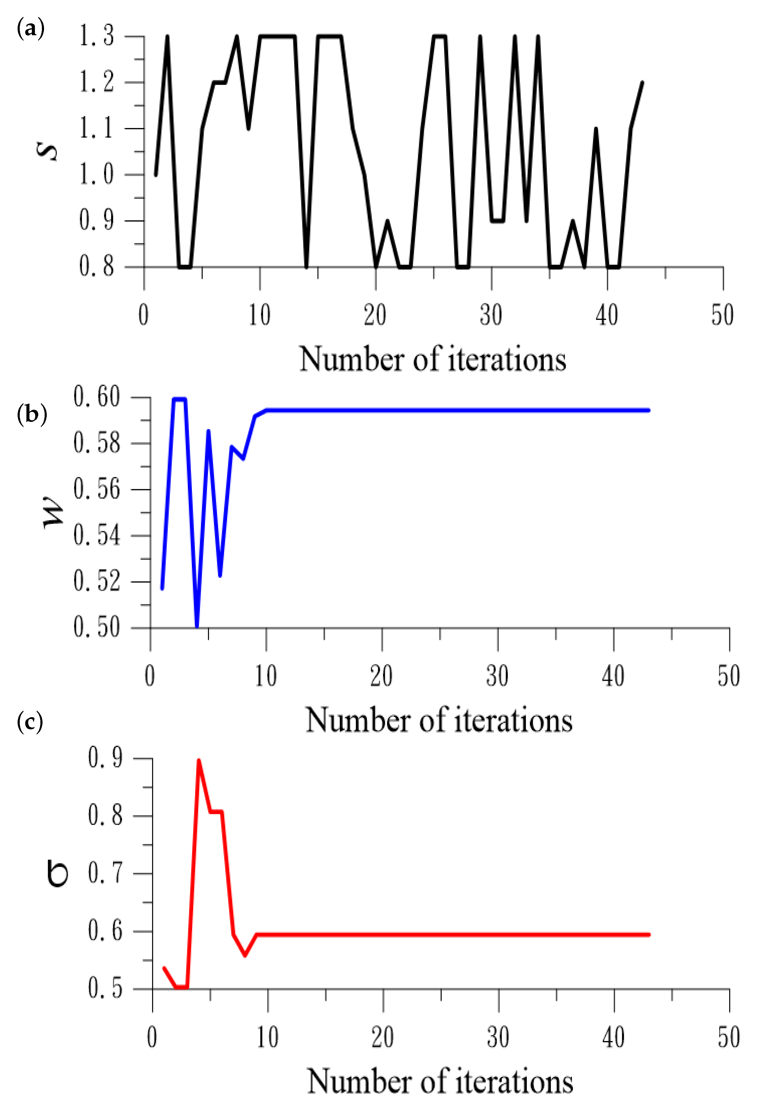
By using OSSAOR, we take ( A , B ) = ( 0.8 , 1.3 ) , ( a , b ) × ( c , d ) = ( 0.5 , 0.6 ) × ( 0.5 , 0.9 ) and ( x 0 , y 0 ) = ( 1 , 1 ) , and NI = 43 under ε = 10 15 is shown in Figure 1a by a dashed line. The solution ( x , y ) = ( 0.163635 , 0.230529 ) is obtained, and ( | F 1 | , | F 2 | ) = ( 3.33 × 10 16 , 0 ) are much smaller than that in [21]. Figure 2a–c reveal s, w and σ . After ten steps, w and σ tend to constant values. For the OSSAOR, COC = 3.67, and the CPU time is 0.29 s.
Starting from an initial value ( x 0 , y 0 ) = ( 10 , 10 ) and under a convergence criterion ε = 10 10 , the OSSAOR converges with NI = 31 to
( x , y ) = ( 0.163635 , 0.230529 ) ,
and the OSSSOR converges with NI = 40 to the same solution. In [14], the double optimal iterative algorithm (DOIA) with NI = 223 tends to
( x , y ) = ( 0.134212 , 0.811128 ) .
On the other hand, the Newton iterative algorithm with NI = 410 converges to
( x , y ) = ( 39.020711 , 38.241665 ) .
Different methods may lead to different solutions; although, they used the same initial guesses.
In Figure 3, we compare the convergence speeds of those four methods, of which OSSSOR and OSSAOR are convergent faster than DOIA and the Newton method.

6.2. Example 2

Next, we apply the OSSSOR and OSSAOR to solve a nonlinear boundary value problem:
u = 3 2 u 2 , u ( 0 ) = 4 , u ( 1 ) = 1 .
The exact solution of Equation (70) is
u ( x ) = 4 ( 1 + x ) 2 .
By introducing a finite difference discretization of u at the grid points, we can obtain
F i = 1 ( Δ x ) 2 ( u i + 1 2 u i + u i 1 ) 3 2 u i 2 = 0 , i = 1 , , n , u 0 = 4 , u n + 1 = 1 ,
where Δ x = 1 / ( n + 1 ) is the grid length.
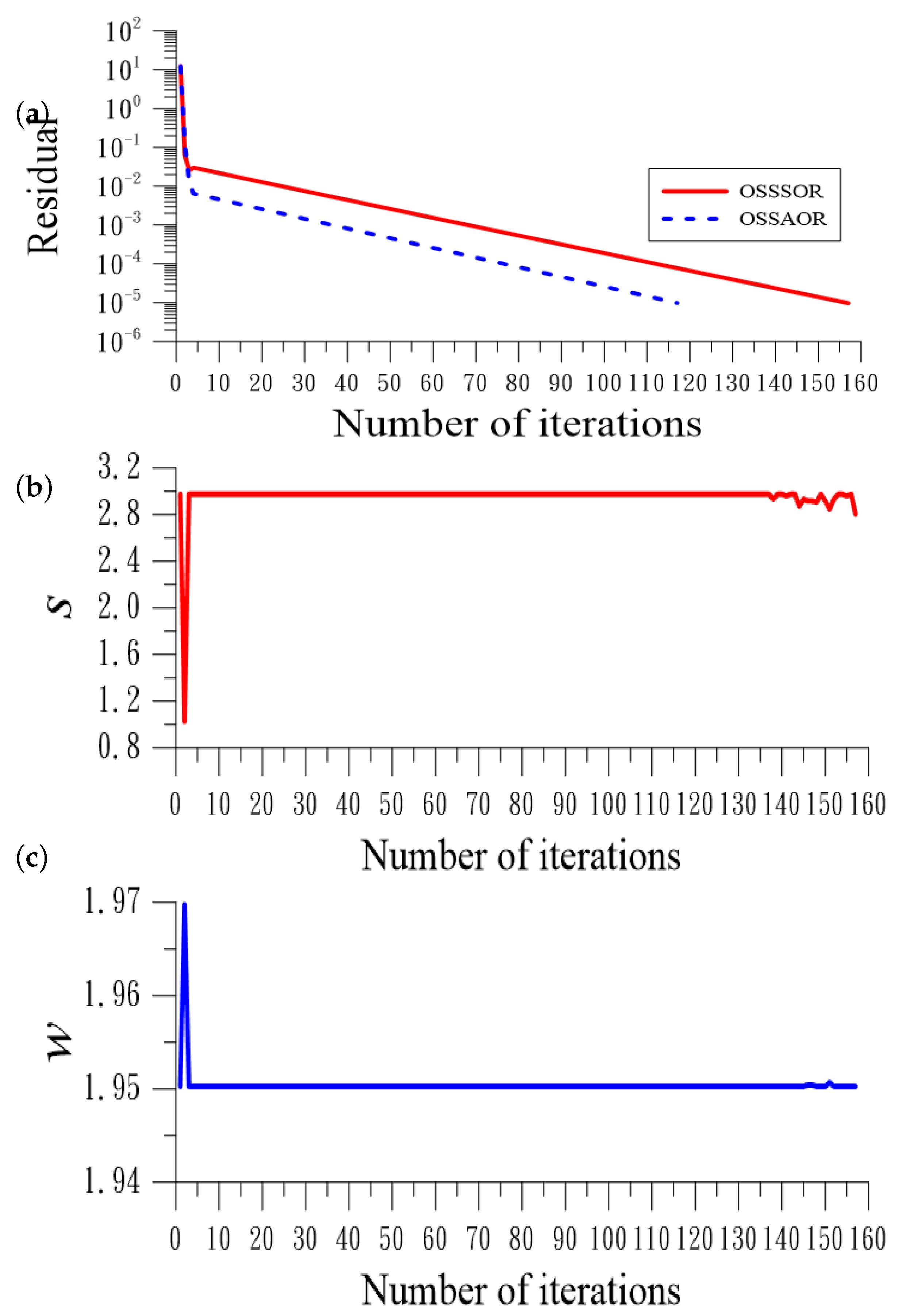
By using OSSSOR, we take n = 89 , ( a , b ) × ( c , d ) = ( 1 , 3 ) × ( 1.95 , 1.97 ) , and NI = 157 under ε = 10 5 is shown in Figure 4a by a solid line. At the final step, the residual 9.06 × 10 11 is obtained. For the OSSSOR, COC = 1.67, and the CPU time is 1.79 s.
Figure 4b,c show s and w. The maximum error (ME) obtained by the OSSSOR is 7.91 × 10 5 . It is convergent faster and more accurate than that obtained in [21], where NI > 8000 under ε = 10 4 and the error is larger than 10 3 .
By using OSSAOR, we take ( A , B ) = ( 0.8 , 1.5 ) , ( a , b ) × ( c , d ) = ( 1.92 , 1.98 ) × ( 1.92 , 1.98 ) , and NI = 117 under ε = 10 5 is shown in Figure 4a by a dashed line, which is convergent faster than the OSSAOR. For the OSSAOR, COC = 1.66, and the CPU time is 1.35 s.
ME obtained by the OSSAOR is 4.03 × 10 5 . In Figure 5a–c, s, w and σ tend to constant values after the first few steps.

6.3. Example 3

We test the following nonlinear Poisson equation by OSSSOR and OSSAOR:
Δ u ( x , y ) + p ( x , y ) u 3 ( x , y ) = 0 , 0 < x < 1 , 0 < y < 1 ,
p ( x , y ) = 4 ( x 2 + y 2 + 9 ) .
The exact solution of Equation (73) is
u ( x , y ) = 1 x 2 + y 2 9 .
Let u i , j k : = u k ( x i , y j ) be a kth step numerical value where ( x i , y j ) = ( i Δ x , j Δ y ) with Δ x = 1 / ( n 1 + 1 ) and Δ y = 1 / ( n 2 + 1 ) . The splitting form of Equation (73) is
Δ u ( x , y ) + s p ( x , y ) u k ( x , y ) 2 u ( x , y ) = ( s 1 ) p ( x , y ) u k ( x , y ) 3 .
Because u k ( x , y ) is obtained at the previous step, Equation (76) is a linear Poisson equation to find the value of u ( x , y ) at the next step.
From Equation (76), the linearized equations are given by
F i , j = 1 ( Δ x ) 2 [ u i + 1 , j 2 u i , j + u i 1 , j ] + 1 ( Δ y ) 2 [ u i , j + 1 2 u i , j + u i , j 1 ] + s p ( x i , y j ) [ u i , j k ] 2 u i , j ( s 1 ) p ( x i , y j ) [ u i , j k ] 3 = 0 , 1 i n 1 , 1 j n 2 ,
where u 0 , j = g 1 ( y j ) = 1 / ( 9 y j 2 ) , u n 1 + 1 , j = g 3 ( y j ) = 1 / ( 8 y j 2 ) , u i , 0 = g 2 ( x i ) = 1 / ( 9 x i 2 ) , and u i , n 2 + 1 = g 4 ( x i ) = 1 / ( 8 x i 2 ) .
Letting K = n 2 ( i 1 ) + j , x K in Equation (23) and F K are computed by
D o i = 1 , n 1 , D o j = 1 , n 2 , K = n 2 ( i 1 ) + j , x K = u i , j , F K = F i , j ,
while b and A are constructed by
D o i = 1 , n 1 , D o j = 1 , n 2 , K = n 2 ( i 1 ) + j , b K = ( s 1 ) p ( x i , y j ) [ u i , j k ] 3 , L 1 = n 2 ( i 2 ) + j , L 2 = n 2 ( i 1 ) + j 1 , L 3 = n 2 ( i 1 ) + j , L 4 = n 2 ( i 1 ) + j + 1 , L 5 = n 2 i + j , A K , L 1 = A K , L 5 = 1 ( Δ x ) 2 , A K , L 2 = A K , L 4 = 1 ( Δ y ) 2 , A K , L 3 = 2 ( Δ x ) 2 2 ( Δ y ) 2 s p ( x i , y j ) [ u i , j k ] 2 .
Here, we have n = n 1 × n 2 equations. For the point on the boundary, we take b k by the given boundary conditions.
By using OSSSOR, we take n = n 1 × n 2 = 20 × 20 , ( a , b ) × ( c , d ) = ( 1 , 3 ) × ( 1.5 , 2 ) , and it converges with NI = 79 under ε = 10 5 as shown in Figure 6a by a solid line. Figure 6b,c show s and w. For the OSSSOR, COC = 1.59, and the CPU time is 13.89 s.
ME obtained by the OSSSOR is 8.73 × 10 6 . It is more accurate than that obtained by Liu [14], whose ME is 5.36 × 10 3 . It is much better than that in [1], which spent over 1000 steps and with ME = 8.57 × 10 3 .
By using OSSAOR, we take ( A , B ) = ( 0.8 , 1.2 ) , ( a , b ) × ( c , d ) = ( 1.7 , 1.8 ) × ( 1.7 , 1.8 ) , and it converges with NI = 51 under ε = 10 5 as shown in Figure 6a by a dashed line. ME obtained by the OSSAOR is 6.62 × 10 6 . Both the convergence speed and accuracy are better than that obtained by the OSSSOR. Figure 7a–c plot s, w and σ . For the OSSAOR, COC = 1.54, and the CPU time is 16.99 s.

6.4. Example 4

An almost linear equations system was given by Brown [22]:
F i = x i + j = 1 n x j ( n + 1 ) , i = 1 , , n 1 ,
F n = j = 1 n x j 1 ,
which has a closed-form solution of x i = 1 , i = 1 , , n .
As demonstarted by Han and Han [23], Brown [22] solved this problem with n = 5 by the Newton iterative algorithm and gave an incorrectly converged solution ( 0.579 , 0.579 , 0.579 , 0.579 , 8.90 ) . For n = 10 and 30, Brown [22] found that the Newton iterative algorithm diverges.
By using OSSSOR, we take n = 10 , x i 0 = 1.5 , i = 1 , , 10 , ( a , b ) × ( c , d ) = ( 1.3 , 1.5 ) × ( 0.5 , 1 ) , and NI = 223 under ε = 10 10 is shown in Figure 8a by a solid line. Figure 8b,c plotted s and w. ME = 9.27 × 10 10 is obtained by the OSSSOR. For the OSSSOR, COC = 1.8 and the CPU time is 1.32 s.
We fix ε = 10 5 and consider different n in the comparison between the Newton method and OSSSOR in Table 1, where the number of iterations (NI) and ME are compared. Table 1 shows that the OSSSOR outperforms the Newton method when n 10 .
Comparing the OSSAOR to OSSSOR, we take n = 10 , which is convergent with NI = 145 under ε = 10 10 as shown in Figure 8a by a dashed line. ME = 3.65 × 10 10 is obtained by the OSSAOR. Both the convergence speed and accuracy are slightly better than that obtained by the OSSSOR.
By using OSSAOR, we take n = 15 , x i 0 = 1.5 , i = 1 , , 15 , ( A , B ) = ( 1.25 , 1.7 ) , ( a , b ) × ( c , d ) = ( 0.2 , 0.5 ) × ( 0.2 , 0.5 ) ; it converges with NI = 91 under ε = 10 5 and obtains ME = 5.64 × 10 5 . The OSSAOR is convergent faster and more accurately than the OSSSOR shown in Table 1. Figure 9a–c plot s, w and σ . For the OSSAOR, COC = 1.68, and the CPU time is 0.58 s.

6.5. Example 5

We test the optimal splitting technique with the Cholesky decomposition [17]:
L L T = H ,
where H is a given m × m positive-definite matrix, and L is a lower triangular matrix with n = ( m + 1 ) m / 2 unknown values. We split the nonlinear matrix equation to
s L k L T = H + ( s 1 ) L k L k T .
Starting from an initial guess L 0 , we apply the iteration
L k + 1 T = ( s L k ) 1 [ H + ( s 1 ) L k L k T ] ,
and the optimal splitting technique to determine s k is given by
min s k ( a , b ) f = s k L k L k T 2 H + ( s k 1 ) L k L k T 2 [ ( s k L k L k T ) · ( H + ( s k 1 ) L k L k T ) ] 2 .
We take the Hilbert matrix with h i j = 1 / ( i + j 1 ) as a demonstrative case. By using the optimal splitting technique, we take m = 4 , n = 10 , ( a , b ) = ( 1.45 , 1.55 ) , and it converges with NI = 39 under ε = 10 15 as shown in Figure 10a. The residual error is very small with L L T H = 9.03 × 10 16 . L obtained is almost exact. Figure 10b,c show f and w; f tends to 1 very fast.
In Table 2, we compare NI, ME and the residual (RES) for different dimension m of the Hilbert matrix, where we fix ε = 10 5 . The data in Table 2 show that the optimal splitting technique can perform well. For m = 25 , COC = 2.35 and the CPU time is 0.42 s.

6.6. Example 6

Finally, we test the LU decomposition [17]:
L U = G ,
where G = [ g i j ] is a given m × m matrix, and L is a lower triangular matrix with unit diagonal elements, and U is an upper triangular matrix. Here, we have n = m 2 unknown values. We apply the splitting–linearizing technique to the pair of iterations:
U k + 1 = ( s L k ) 1 [ G + ( s 1 ) L k U k ] ,
L k + 1 = [ G + ( s 1 ) L k U k ] ( s U k ) 1 .
We take g i j = i + 2 j as a demonstrative case. By using the optimal splitting technique, we take m = 6 , n = 36 , ( a , b ) = ( 1.6 , 2.2 ) , and NI = 69 under ε = 10 12 is shown in Figure 11a. The residual error is quite small with L U G = 8.04 × 10 13 . L and U obtained are almost exact. Figure 11b,c show f and w; f tends to 1 very fast. For the optimal splitting technique, COC = 4.47 and the CPU time is 0.34 s.

7. Conclusions

In the paper, the nonlinear terms in the nonlinear equations were decomposed at two sides through a splitting parameter. Then we linearized the nonlinear equations around the values at the previous step and derived a step-by-step linear system to determine the values at the next step. In doing so, we do not need to compute the Jacobian matrix and its inversion at each iteration step. We have combined the splitting technique to the classical methods SSOR and SAOR, whose parameters are optimized by using the maximal projection methods. In summary, the key outcomes of the proposed optimal splitting SSOR (OSSSOR) and optimal splitting SAOR (OSSAOR) are pointed out as follows.
  • There are two parameters in the OSSSOR, while that in the OSSAOR, there are three.
  • Using the maximal projection technique, we derived optimal values of the parameters in the OSSSOR and OSSAOR to accelerate the convergence speed.
  • Searching the minimization in a preferred range is easily performed through a few operations in the golden section search algorithms.
  • The new methods could provide a good choice of the optimal values of the parameters at each iteration.
  • Numerical tests indicated that the OSSAOR is convergent faster than the OSSSOR; however, the OSSAOR is more expensive than the OSSSOR to compute three parameters.
  • The proposed OSSSOR and OSSAOR can provide very accurate solutions through a few iterations, as reflected in the very small value of the residual, and the high values of COC.
It is significant that the SSOR and SAOR are for the first time automatically merged into the new methods of OSSSOR and OSSAOR without needing the inner iterations loop; they are low in computational complexity and save a lot of CPU time. The main difficulties in the SSOR and SAOR are some of the involved parameters; we overcame this difficulty in the paper by choosing the proper values of parameters, speeding up the convergence. In the future, the same idea may be extended to the nonlinear matrix equations, like as the Riccati matrix equation, and many other nonlinear matrix equations.

Author Contributions

Conceptualization, C.-S.L. and C.-W.C.; Methodology, C.-S.L. and C.-W.C.; Software, C.-S.L. and C.-W.C.; Validation, C.-S.L., E.R.E.-Z. and C.-W.C.; Formal analysis, C.-S.L. and C.-W.C.; Investigation, C.-S.L., E.R.E.-Z. and C.-W.C.; Resources, E.R.E.-Z. and C.-W.C.; Data curation, C.-S.L., E.R.E.-Z. and C.-W.C.; Writing—original draft, C.-S.L. and C.-W.C.; Writing—review & editing, C.-S.L. and C.-W.C.; Visualization, C.-S.L., E.R.E.-Z. and C.-W.C.; Supervision, C.-S.L. and C.-W.C.; Project administration, C.-W.C.; Funding acquisition, C.-W.C. All authors have read and agreed to the published version of the manuscript.

Funding

This work was financially supported by the National Science and Technology Council [grant numbers: NSTC 112-2221-E-239-022].

Data Availability Statement

The data presented in this study are available on request from the corresponding authors.

Acknowledgments

E.R.E.-Z. extends their appreciation to Deputyship for Research and Innovation, Ministry of Education, in Saudi Arabia, where this study is supported via funding from Prince sattam bin Abdulaziz University project number (PSAU/2024/R/1445). C.-W.C. was financially supported by the National Science and Technology Council [grant numbers: NSTC 112-2221-E-239-022].

Conflicts of Interest

The authors declare no conflicts of interest.

Appendix A

In this appendix, we give the two-dimensional golden section search algorithm (GSSA) to find the minimum of a give function f ( x , y ) , ( x , y ) [ A , B ] × [ C , D ] with a given stopping criterion ε = 0.01 :
R = [ 5 1 ] / 2 X 1 = A + ( 1 R ) ( B A ) X 2 = A + R ( B A ) Y 1 = C + ( 1 R ) ( D C ) Y 2 = C + R ( D C ) F 11 = f ( X 1 , Y 1 ) F 12 = f ( X 1 , Y 2 ) F 21 = f ( X 2 , Y 1 ) F 22 = f ( X 2 , Y 2 ) F M I N = min ( F 11 , F 11 , F 21 , F 22 ) I f ( B A ) 2 + ( D C ) 2 < ε Then If ( F M I N . E Q . F 11 ) Then f min = F 11 x min = X 1 y min = Y 1 Endif If ( F M I N . E Q . F 12 ) Then f min = F 12 x min = X 1 y min = Y 2 Endif If ( F M I N . E Q . F 21 ) Then f min = F 21 x min = X 2 y min = Y 1 Endif If ( F M I N . E Q . F 22 ) Then f min = F 22 x min = X 2 y min = Y 2 Endif Stop Endif If ( F M I N . E Q . F 11 ) Then B = X 2 D = Y 2 Endif If ( F M I N . E Q . F 12 ) Then B = X 2 C = Y 1 Endif If ( F M I N . E Q . F 22 ) Then A = X 1 C = Y 1 Endif If ( F M I N . E Q . F 21 ) Then A = X 1 D = Y 2 Endif X 1 = A + ( 1 R ) ( B A ) X 2 = A + R ( B A ) Y 1 = C + ( 1 R ) ( D C ) Y 2 = A 2 + R ( D C ) F 11 = f ( X 1 , Y 1 ) F 12 = f ( X 1 , Y 2 ) F 21 = f ( X 2 , Y 1 ) F 22 = f ( X 2 , Y 2 ) F M I N = min ( F 11 , F 12 , F 21 , F 22 )

References

  1. Liu, C.S. A manifold-based exponentially convergent algorithm for solving non-linear partial differential equations. J. Mar. Sci. Tech. 2012, 20, 441–449. [Google Scholar]
  2. Ahmad, F.; Tohidi, E.; Carrasco, J.A. A parameterized multi-step Newton method for solving systems of nonlinear equations. Numer. Algorithms 2016, 71, 631–653. [Google Scholar] [CrossRef]
  3. Ullah, M.Z.; Serra-Capizzano, S.; Ahmad, F. An efficient multi-step iterative method for computing the numerical solution of systems of nonlinear equations associated with ODEs. Appl. Math. Comput. 2015, 250, 249–259. [Google Scholar] [CrossRef]
  4. Ahmad, F.; Tohidi, E.; Ullah, M.Z.; Carrasco, J.A. Higher order multi-step Jarratt-like method for solving systems of nonlinear equations: Application to PDEs and ODEs. Comput. Math. Appl. 2015, 70, 624–636. [Google Scholar] [CrossRef]
  5. Budzko, D.; Cordero, A.; Torregrosa, J.R. Modifications of Newton’s method to extend the convergence domain. SeMA J. 2014, 66, 2254–3902. [Google Scholar] [CrossRef]
  6. Qasima, S.; Ali, Z.; Ahmadb, F.; Serra-Capizzano, S.; Ullah, M.Z.; Mahmoode, A. Solving systems of nonlinear equations when the nonlinearity is expensive. Comput. Math. Appl. 2016, 71, 1464–1478. [Google Scholar] [CrossRef]
  7. AL-Obaidi, R.H.; Darvish, M.T. A comparative study on qualification criteria of nonlinear solvers with introducing some new ones. J. Math. 2022, 2022, 4327913. [Google Scholar] [CrossRef]
  8. Capdevila, R.R.; Cordero, A.; Torregrosa, J.R. Convergence and dynamical study of a new sixth order convergence iterative scheme for solving nonlinear systems. AIMS Math. 2023, 8, 12751–12777. [Google Scholar] [CrossRef]
  9. Qureshi, S.; Chicharro, F.I.; Argyros, I.K.; Soomro, A.; Alahmadi, J.; Hincal, E. A new optimal numerical root-solver for solving systems of nonlinear equations using local, semi-local, and stability analysis. Axioms 2024, 13, 341. [Google Scholar] [CrossRef]
  10. Quarteroni, A.; Sacco, R.; Saleri, F. Numerical Mathematics; Springer Science: New York, NY, USA, 2000. [Google Scholar]
  11. Hadjidimos, A. Accelerated overrelaxation method. Math. Comput. 1978, 32, 149–157. [Google Scholar] [CrossRef]
  12. Hadjidimos, A.; Yeyios, A. Symmetric accelerated overrelaxation (SAOR) method. Math. Comput. Simul. 1982, XXIV, 72–76. [Google Scholar] [CrossRef]
  13. Hadjidimos, A. Successive overrelaxation (SOR) and related methods. J. Comput. Appl. Math. 2000, 123, 177–199. [Google Scholar] [CrossRef]
  14. Liu, C.S. A double optimal iterative algorithm in an affine Krylov subspace for solving nonlinear algebraic equations. Comput. Math. Appl. 2015, 70, 2376–2400. [Google Scholar] [CrossRef]
  15. Yeyios, A. A necessary condition for the convergence of the accelerated overrelaxation (AOR) method. J. Comput. Appl. Math. 1989, 26, 371–373. [Google Scholar] [CrossRef]
  16. Yeih, W.; Chan, I.Y.; Ku, C.Y.; Fan, C.M.; Guan, P.C. A double iteration process for solving the nonlinear algebraic equations, especially for ill-posed nonlinear algebraic equations. Comput. Model. Eng. Sci. 2014, 99, 123–149. [Google Scholar]
  17. Golub, G.H.; Van Loan, C.F. Matrix Computations; The Johns Hopkins University Press: Baltimore, MD, USA, 1996. [Google Scholar]
  18. Liu, C.S.; El-Zahar, E.R.; Chang, C.W. Dynamical optimal values of parameters in the SSOR, AOR and SAOR testing using the Poisson linear equations. Mathematics 2023, 11, 3828. [Google Scholar] [CrossRef]
  19. Hirsch, M.; Smale, S. On algorithms for solving f(x)=0. Commun. Pure Appl. Math. 1979, 32, 281–312. [Google Scholar] [CrossRef]
  20. Liu, C.S.; Atluri, S.N. A novel time integration method for solving a large system of non-linear algebraic equations. Comput. Model. Eng. Sci. 2008, 31, 71–83. [Google Scholar]
  21. Atluri, S.N.; Liu, C.S.; Kuo, C.L. A modified Newton method for solving non-linear algebraic equations. J. Marine Sci. Tech. 2009, 17, 238–247. [Google Scholar] [CrossRef]
  22. Brown, K.M. Computer oriented algorithms for solving systems of simultaneous nonlinear algebraic equations. In Numerical Solution of Systems of Nonlinear Algebraic Equations; Byrne, G.D., Hall, C.A., Eds.; Academic Press: New York, NY, USA, 1973; pp. 281–348. [Google Scholar]
  23. Han, T.; Han, Y. Solving large scale nonlinear equations by a new ODE numerical integration method. Appl. Math. 2010, 1, 222–229. [Google Scholar] [CrossRef]
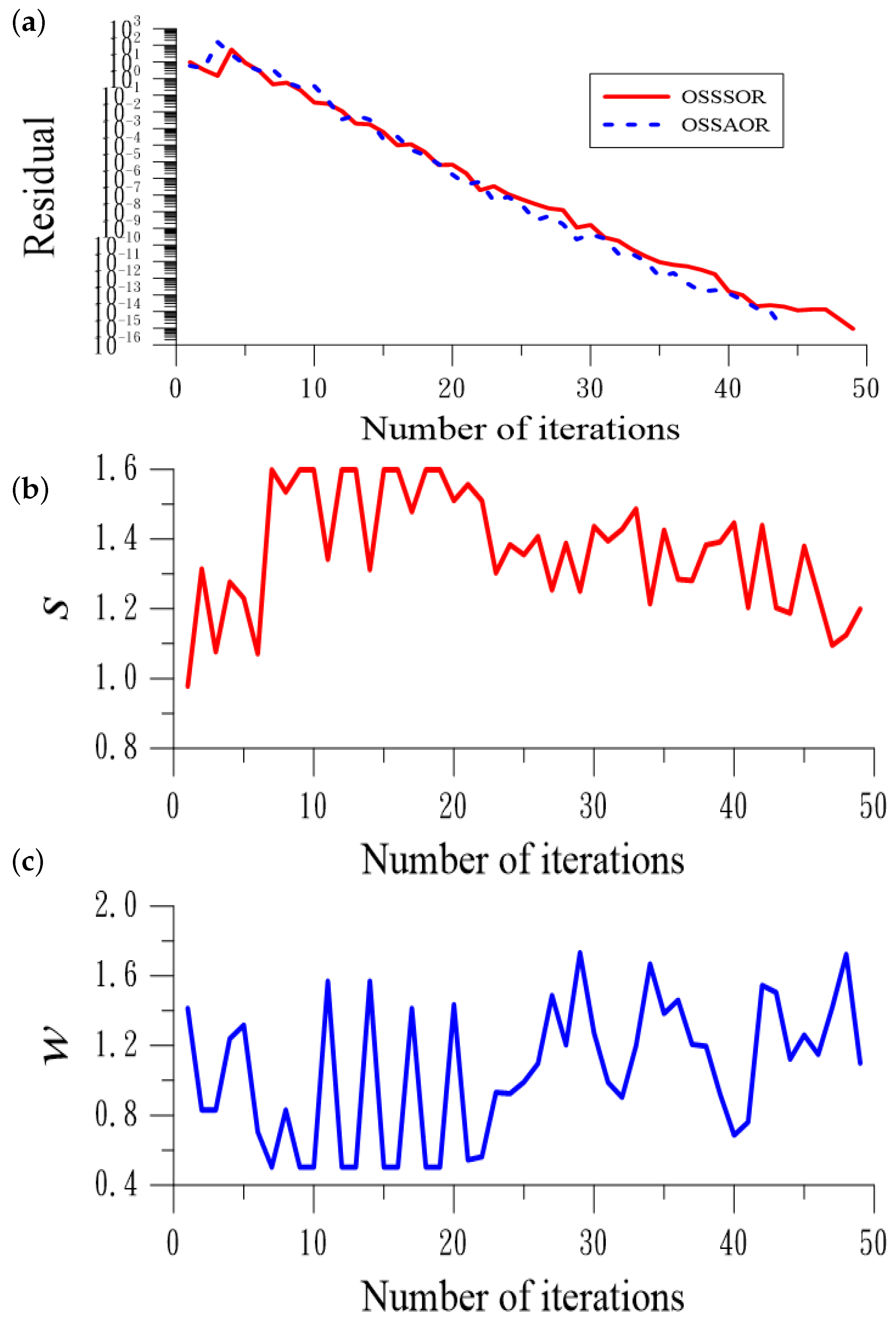
Figure 1. For example 1 of nonlinear equations solved by OSSSOR, (a) showing residuals, (b) optimal splitting parameters and (c) optimal relaxation parameters.
Mathematics 12 01808 g001
Figure 2. For example 1 of nonlinear equations solved by OSSAOR, (a) optimal splitting parameters, (b) optimal relaxation parameters and (c) optimal accelerating parameters.
Mathematics 12 01808 g002
Figure 3. For example 1 of nonlinear equations solved by four different methods comparing the convergence speeds.
Mathematics 12 01808 g003
Figure 4. For example 2 of nonlinear equations solved by OSSSOR, (a) showing residuals, (b) optimal splitting parameters and (c) optimal relaxation parameters.
Mathematics 12 01808 g004
Figure 5. For example 2 of nonlinear equations solved by OSSAOR, (a) optimal splitting parameters, (b) optimal relaxation parameters and (c) optimal accelerating parameters.
Mathematics 12 01808 g005aMathematics 12 01808 g005b
Figure 6. For example 3 of nonlinear equations solved by OSSSOR, (a) showing residuals, (b) optimal splitting parameters and (c) optimal relaxation parameters.
Mathematics 12 01808 g006aMathematics 12 01808 g006b
Figure 7. For example 3 of nonlinear equations solved by OSSAOR, (a) optimal splitting parameters, (b) optimal relaxation parameters and (c) optimal accelerating parameters.
Mathematics 12 01808 g007
Figure 8. For example 4 of nonlinear equations solved by OSSSOR, (a) showing residuals, (b) optimal splitting parameters and (c) optimal relaxation parameters.
Mathematics 12 01808 g008
Figure 9. For example 4 of nonlinear equations solved by OSSAOR, (a) optimal splitting parameters, (b) optimal relaxation parameters and (c) optimal accelerating parameters.
Mathematics 12 01808 g009
Figure 10. For the Cholesky decomposition of a Hilbert matrix, (a) residuals, (b) merit function and (c) optimal splitting parameters.
Mathematics 12 01808 g010
Figure 11. For the LU decomposition, (a) residuals, (b) merit function and (c) optimal splitting parameters.
Mathematics 12 01808 g011aMathematics 12 01808 g011b
Table 1. For Brown’s problem with different dimension n, comparing the performance of Newton method and OSSSOR.
n45671015
NI (Newton)1215158>1000>1000
NI (OSSSOR)28415571134199
ME (Newton) 8.15 × 10 9 7.9 5.42 × 10 6 11.591015
ME (OSSSOR) 1.32 × 10 5 1.2 × 10 5 3.66 × 10 5 6.84 × 10 5 2.92 × 10 5 1.14 × 10 4
Table 2. For the Cholesky decomposition equation of the Hilbert matrices with different dimension m, comparing NI, ME and RES.
m3510152025
NI131725323842
ME 3.59 × 10 6 3.90 × 10 6 3.07 × 10 6 2.09 × 10 6 1.48 × 10 6 1.69 × 10 6
RES 5.45 × 10 6 5.79 × 10 6 8.19 × 10 6 6.77 × 10 6 7.78 × 10 6 7.97 × 10 6
Disclaimer/Publisher’s Note: The statements, opinions and data contained in all publications are solely those of the individual author(s) and contributor(s) and not of MDPI and/or the editor(s). MDPI and/or the editor(s) disclaim responsibility for any injury to people or property resulting from any ideas, methods, instructions or products referred to in the content.