Lambert W Functions in the Analysis of Nonlinear Dynamics and Bifurcations of a 2D γ-Ricker Population Model

Abstract

The aim of this paper is to study the use of Lambert W functions in the analysis of nonlinear dynamics and bifurcations of a new two-dimensional $\gamma$-Ricker population model. Through the use of such transcendental functions, it is possible to study the fixed points and the respective eigenvalues of this exponential diffeomorphism as analytical expressions. Consequently, the maximum number of fixed points is proved, depending on whether the Allee effect parameter $\gamma$ is even or odd. In addition, the analysis of the bifurcation structure of this $\gamma$-Ricker diffeomorphism, also taking into account the parity of the Allee effect parameter, demonstrates the results established using the Lambert W functions. Numerical studies are included to illustrate the theoretical results.

1. Introduction and Motivation

The Ricker population growth model is one of the most well-known models in population ecology and biology, which describes how the size of a population evolves over time. The linear growth model assumes a constant increase in population over time, whereas the Ricker model incorporates population self-regulation, rendering it nonlinear. The nonlinear dynamics of the Ricker population growth model are expressed by the population growth rate being inversely proportional to the population size, i.e., the growth rate decreases as the population density increases, reflecting competition for finite resources (see [1]). Inspired by the Ricker population model, various population growth models adapted to specific realities and with different purposes have been proposed in recent decades (see [2,3,4] and references therein).

In particular, we consider the $\gamma$-Ricker population model whose dynamics of the population $x_n$, after $n\in \mathbb{N}$ generations, are defined by the difference equation,

$$x_{n+1}=b\left(x_n\right)x_{n}s\left(x_n\right)=r{x}_n^{\gamma }{e}^{-\delta x_n},$$

(1)

where $b\left(x_n\right)=x_n^{\gamma -1}$ is the per capita birth or growth function, i.e., a cooperation or interference factor, with $\gamma$ the cooperation parameter or Allee effect parameter, $s\left(x_n\right)=e^{\mu -\delta x_n}$ is the survival function for generation n or the intraspecific competition, with $\mu$ the density-independent death rate $(r=e^{\mu })$, and $\delta$ the carrying capacity parameter.

The purpose of this work is to investigate the nonlinear dynamics of a new class of “continuous” embedding of the one-dimensional (1D for short) $\gamma$-Ricker population model into a two-dimensional (2D for short) diffeomorphism. We consider a 2D $\gamma$-Ricker diffeomorphism, $T_b:{\mathbb{R}}^2\to {\mathbb{R}}^2$, which is defined by the following recurrence equations:

$$T_b\equiv \left\{\begin{array}{c}{x}_{n+1}=f(x_n;r,\gamma ,\delta )+y_n\hfill \\ y_{n+1}=b{x}_n\hfill \end{array}\right.\iff$$

$$T_b\equiv \left\{\begin{array}{c}{f}_1(x_n,y_n;r,\gamma ,\delta ,b)=r{x}_n^{\gamma }{e}^{-\delta x_n}+y_n\hfill \\ f_2(x_n,y_n;r,\gamma ,\delta ,b)=b{x}_n\hfill \end{array}\right.,$$

(2)

where $b\in \mathbb{R}\setminus \left\{0\right\}$ is the embedding parameter, $(x_n,y_n)\in {\mathbb{R}}^2$ and $n\in \mathbb{N}$. This 2D or planar map $T_b$ is defined in a parameters space, which is given by,

$${\Sigma }_b=\left\{(r,\gamma ,\delta ,b)\in {\mathbb{R}}^4:r\ne 0,\gamma \in \mathbb{N},\delta \ne 0,\left|b\right|\le 1\right\}.$$

(3)

We remark that the particular case $b=0$ ($T_0$) has already been studied in [2], which corresponds to the classical 1D $\gamma$-Ricker population model. From the population dynamics point of view, the 2D diffeomorphism $T_b$, given by Equation (2), describes an interaction between two population species $x_n$ and $y_n$, which are related to each other through the planar system $T_b$, such that $T_0$ is the 1D $\gamma$-Ricker population model, given by Equation (1), in some parameters space. Thus, in the analyzed case throughout this work, it is said that the 1D $\gamma$-Ricker population model is embedded into the 2D invertible map or exponential diffeomorphism $T_b$. As in several references cited throughout this work, the knowledge of the behaviour of nonlinear dynamics and the bifurcation structures of the 1D $\gamma$-Ricker population model $T_0$ gives us a “germinal” state for understanding the performance of the nonlinear dynamics and bifurcations of the 2D exponential diffeomorphism $T_b$, for sufficiently small b-values. The study of diffeomorphisms from a bifurcation theory point of view has been extensively analyzed by Mira in [5] (see also [6,7,8,9,10,11,12] and references therein).

The structure of this paper is as follows: In Section 2, we establish explicit expressions for the fixed points of the 2D $\gamma$-Ricker diffeomorphism $T_b$, defining them as analytical solutions of Lambert W functions. Given the complexity of the problem, as far as the behaviour of the Allee effect parameter $\gamma$ is concerned, we will carry out our analysis in two separate cases, the odd and even cases. The nature and stability of the fixed points are studied in Section 3. This analysis is carried out by separating the trivial fixed point from the other fixed points. In particular, in the case of nontrivial fixed points, the associated eigenvalues are written as Lambert W functions, thus revealing the complexity of the 2D model being analyzed. In Section 4, the fold and flip global bifurcations of the 2D $\gamma$-Ricker diffeomorphism $T_b$ are studied. This study is based on the use of contour lines related to a k-cycle of $T_b$, with $k\in \mathbb{N}$. Similarly to Section 2, the investigation of bifurcation structures of $T_b$ in a parameter plane will be performed by considering the Allee effect parameter odd or even separately. In particular, the numerical cases explored in this section confirm and illustrate the theoretical results of the previous sections. Finally, in Section 5, we discuss our work and provide some relevant conclusions, presenting some future research perspectives in this area. This study presents the results of numerical simulations conducted in Mathematica, Maple, Fortran and Python.

2. Lambert $\mathit{W}$ Functions as Analytical Solutions of the Fixed Points of ${\mathbf{T}}_{\mathbf{b}}$

In this section, we will study the existence of fixed points of the 2D $\gamma$-Ricker diffeomorphism $T_b$. We will see that the trivial fixed point $(x_0^{*},y_0^{*})=(0,0)$ exists for all $\gamma \in \mathbb{N}$ and we will define, in Propositions 1 and 2, conditions for the existence of other fixed points.

For simplification, we will use the following notation from now on:

$$T_b(x,y)=\left(f_1\left(x,y;r,\gamma ,\delta ,b\right),f_2\left(x,y;r,\gamma ,\delta ,b\right)\right),$$

(4)

where $f_1$ and $f_2$ are defined as in Equation (2).

The fixed points of $T_b$ are obtained by solving the next system,

$$\left\{\begin{array}{c}{f}_1(x,y;r,\gamma ,\delta ,b)=x\hfill \\ f_2(x,y;r,\gamma ,\delta ,b)=y\hfill \end{array}\right.\iff \left\{\begin{array}{c}r{x}^{\gamma }{e}^{-\delta x}+y=x\hfill \\ bx=y\hfill \end{array}\right..$$

(5)

The previous system is reduced to an equation only in the variable x, given by,

$$r{x}^{\gamma }{e}^{-\delta x}+bx=x.$$

(6)

So, we are going to introduce a real function, only in the variable x, $F_b:\mathbb{R}\to \mathbb{R}$, defined by,

$$F_b\left(x;r,\gamma ,\delta \right)=r{x}^{\gamma }{e}^{-\delta x}+bx,$$

(7)

whose equation of its fixed points corresponds to a reduction of the system given by Equation (5), in 2D, to a problem of determining fixed points in 1D. However, the equation of the fixed points of $F_b$, given by Equation (7), is an implicit equation in the variable x.

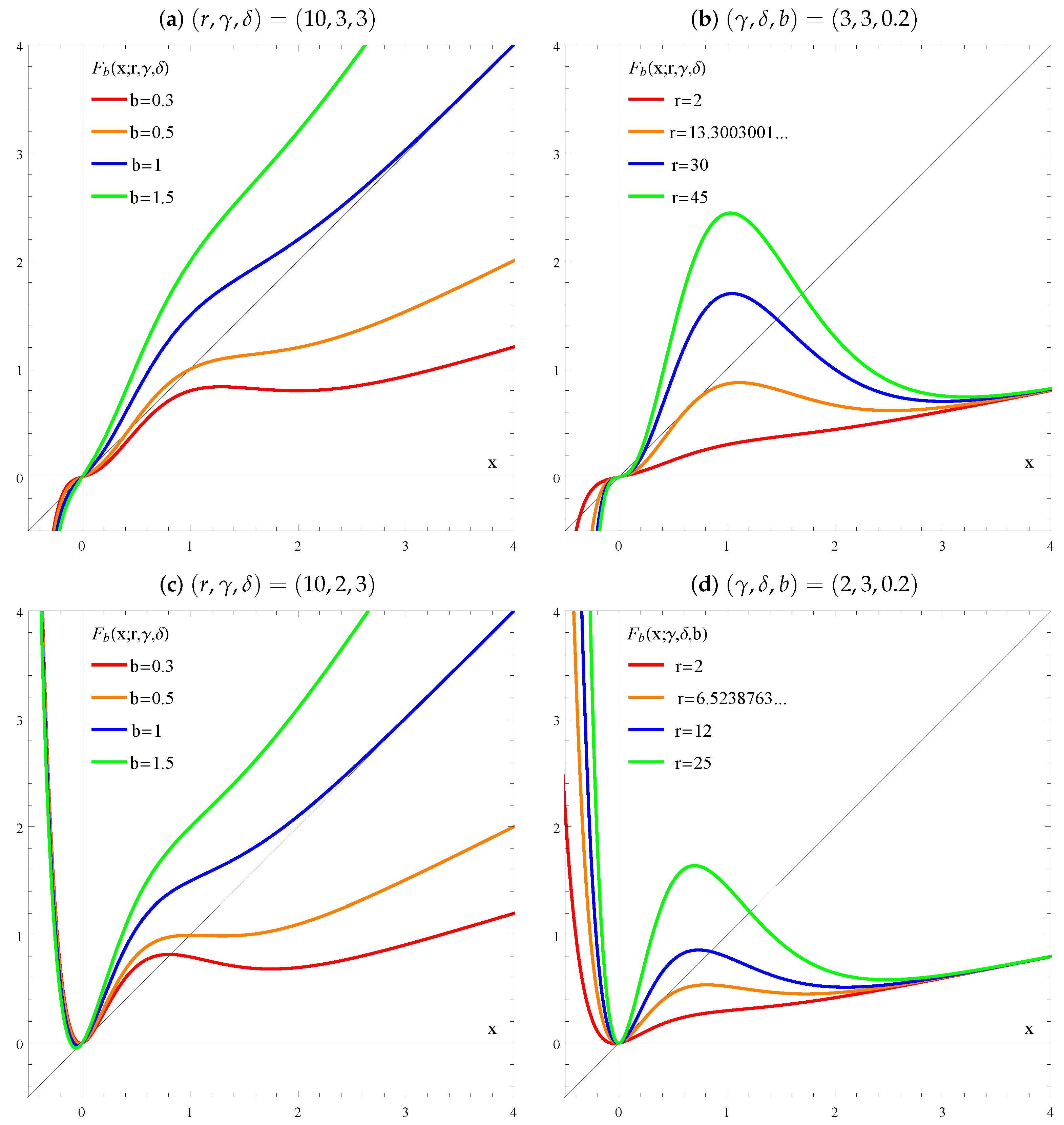
Some graphics of $F_b$ are plotted in Figure 1 for certain parameter values at ${\Sigma }_b$. We can see that in Figure 1a, according to the variation in the parameter b and for the fixed parameters $(r,\gamma ,\delta )=(10,3,3)$ ($\gamma =3$ is odd), there is always the fixed point $(0,0)$, but there may also be three nonzero fixed points (orange graphic) or a negative solution (red graphic). Note that the case $b=1$ (blue graphic) represents an asymptotic behaviour only with the fixed point $(0,0)$. The green graphic $(b=1.5)$ also only admits the $(0,0)$ fixed point. On the other hand, Figure 1b ($\gamma =3$ is odd) shows the usual behaviour of an Allee effect function, for $x>0$, according to the variation in the parameter r and for the fixed parameters $(\gamma ,\delta ,b)=(3,3,0.2)$. In this case, all the examples of $F_b$ have a negative fixed point and the blue and green graphics $(r=30,45)$ have four fixed points. For the class of Allee effect functions, the fixed point (0,0) always exists, and a fold bifurcation creates two nonzero fixed points. For more details on Allee effect functions see, for example, [2,13] and references therein. Figure 1c ($\gamma =2$ is even) depicts graphics of $F_b$ where there is a single fixed point $(0,0)$, which is the blue graphic, two fixed points ($(0,0)$ and one negative), which is the green graphic, and three fixed points corresponding to the orange and red graphics ($(0,0)$ and two positive fixed points). Figure 1d ($\gamma =2$ is even) shows examples of Allee effect functions, where the negative fixed point does not exist, the fixed point $(0,0)$ always exists and there are at most two positive fixed points (blue and green graphics).

The previous numerical simulations suggest that the system given by Equation (5) may, in some cases, have at least the $(0,0)$ solution and at most four fixed points. In the case of four fixed points, we have identified the null solution, two positive fixed points and one negative fixed point, or the vice versa case. Note that, for some parameter values $(r,\gamma ,\delta ,b)\in {\Sigma }_b$, the following property is verified.

Property 1.

Let $F_b:\mathbb{R}\to \mathbb{R}$ be the real function defined by Equation (7). In the ${\Sigma }_b$ parameters space, if $\gamma =2n+1$, then the following property holds true:

$$F_b\left(x;r,\gamma ,\delta \right)=-F_b\left(-x;r,\gamma ,-\delta \right).$$

The result of Property 1 was identified in [14] as a mirror symmetric map, in the context of kneading theory. Note that, using Property 1, we may conclude that if x is a fixed point of $F_b(x;r,\gamma ,\delta )$, then $-x$ is a fixed point of $F_b(x;r,\gamma ,-\delta )$, for $\gamma =2n+1$, because it turns out,

$$F_b(x;r,\gamma ,\delta )=x\iff -F_b(-x;r,\gamma ,-\delta )=x\iff F_b(-x;r,\gamma ,-\delta )=-x.$$

This result shows that in the case $\gamma =2n+1$, there is a special behaviour in the existence of the fixed points of $T_b$ and consequently in the associated bifurcation structures, as can be seen in the results presented in Section 2.1 and Section 4.1.

Throughout this work, we will consider the set of the fixed points of $T_b$ in ${\mathbb{R}}^2$ denoted by $X^{*}$. The main result of this work is the following theorem, which establishes the maximum number of fixed points of $T_b$:

Theorem 1.

Let $T_b:{\mathbb{R}}^2\to {\mathbb{R}}^2$ be the 2D γ-Ricker diffeomorphism defined by Equation (4). In the $(X^{*},{\Sigma }_b)$ space, the following properties hold true:

(i) 

if $\gamma =2n+1$, then $T_b$ has a maximum of four fixed points;

(ii) 

if $\gamma =2n$, then $T_b$ has a maximum of three fixed points.

The result of Theorem 1 will be proved over the next few sections, where various cases will be analyzed. Considering the structure of the system for determining the fixed points of $T_b$, given by Equation (5), and the numerical results provided by Equation (7), where some examples are illustrated in Figure 1, we use the Lambert W functions to support this study.

In this work, we consider the Lambert W function as the real analytic inverse of the function $y=x{e}^x$. The inverse is defined only for $x\ge -\frac{1}{e}$ and is double-valued at the point $\left(-\frac{1}{e},-1\right)$. The real branches of the Lambert W function are denoted by $W_0$ and $W_{-1}$. Branch $W_0$ is referred to as the principal branch, which is increasing for $W\left(x\right)\ge -1$, and the lower branch is denoted by $W_{-1}\left(x\right)$, which is decreasing from $W_{-1}(-\frac{1}{e})=-1$ to $W_{-1}\left(0^{-}\right)=-\infty$ (see Figure 2). The Lambert W function is associated with the logarithmic function and arises from many models in the natural sciences, where we can mention a vast diversity of applications and problems in physics, biological, ecological and evolutionary models (see [15]). For more details and applications of the Lambert W function, see, for example, [2,3,4,16,17,18,19,20] and references therein. However, the complexity of problems involving transcendental functions of this type have evolved and in parallel new and more complex functions have been defined and developed in this category, namely, the generalised Lambert W function. For more details on this subject, see [21,22,23,24,25,26].

For $\gamma \in \mathbb{N}$, the system given by Equation (5) is written in equivalent form as follows:

$$\left\{\begin{array}{c}x=0\hfill \\ y=0\hfill \end{array}\right.\vee \left\{\begin{array}{c}r{x}^{\gamma -1}{e}^{-\delta x}+b=1\hfill \\ y=bx\hfill \end{array}\right..$$

(8)

So, we established the first result about the fixed points of $T_b$.

Property 2.

Let $T_b:{\mathbb{R}}^2\to {\mathbb{R}}^2$ be the 2D γ-Ricker diffeomorphism defined by Equation (4). In the $(X^{*},{\Sigma }_b)$ space, the point $(x_0^{*},y_0^{*})=(0,0)$ is always a fixed point of $T_b$.

The existence of nontrivial fixed points will be studied in two separate cases: case I, for $\gamma =2n+1$, and case II, for $\gamma =2n$. We remark that, the particular cases $\gamma =1$ and $b=1$ will be analyzed throughout this work.

2.1. Case I: $\gamma =2n+1$

Now, we will focus on analyzing Equation (8), when $\gamma =2n+1$, i.e., $\gamma$ is an odd natural number $(\gamma -1=2n)$. In this case, the nonzero solutions given by Equation (8) are written as follows:

$$\left\{\begin{array}{c}r{x}^{\gamma -1}{e}^{-\delta x}=1-b\hfill \\ y=bx\hfill \end{array}\right.\iff \left\{\begin{array}{c}{r}^{\frac{1}{\gamma -1}}\left|x\right|e^{-\frac{\delta }{\gamma -1}x}={\left(1-b\right)}^{\frac{1}{\gamma -1}}\hfill \\ y=bx\hfill \end{array}\right..$$

(9)

Equivalently, we have the following equalities:

$$\left\{\begin{array}{c}x{e}^{-\frac{\delta }{\gamma -1}x}={\left(\frac{1-b}{r}\right)}^{\frac{1}{\gamma -1}},\mathrm{if}x>0\hfill \\ \\ x{e}^{-\frac{\delta }{\gamma -1}x}=-{\left(\frac{1-b}{r}\right)}^{\frac{1}{\gamma -1}},\mathrm{if}x<0\hfill \\ \\ y=bx\hfill \end{array}\right.$$

$$\iff \left\{\begin{array}{c}-\frac{\delta }{\gamma -1}x{e}^{-\frac{\delta }{\gamma -1}x}=-\frac{\delta }{\gamma -1}{\left(\frac{1-b}{r}\right)}^{\frac{1}{\gamma -1}},\mathrm{if}x>0\hfill \\ \\ -\frac{\delta }{\gamma -1}x{e}^{-\frac{\delta }{\gamma -1}x}=\frac{\delta }{\gamma -1}{\left(\frac{1-b}{r}\right)}^{\frac{1}{\gamma -1}},\mathrm{if}x<0\hfill \\ \\ y=bx\hfill \end{array}\right..$$

(10)

In a simplified form, the equations given by Equation (10) can be presented as follows:

$$\left\{\begin{array}{c}X{e}^X=-\frac{\delta }{\gamma -1}{\left(\frac{1-b}{r}\right)}^{\frac{1}{\gamma -1}},\mathrm{if}x>0\mathrm{and}x=-\frac{\gamma -1}{\delta }X\hfill \\ \\ X{e}^X=\frac{\delta }{\gamma -1}{\left(\frac{1-b}{r}\right)}^{\frac{1}{\gamma -1}},\mathrm{if}x<0\mathrm{and}x=-\frac{\gamma -1}{\delta }X\hfill \\ \\ y=bx\hfill \end{array}\right..$$

(11)

Thus, we can establish that the equation given by,

$$r{x}^{\gamma -1}{e}^{-\delta x}=1-b,$$

(12)

in Equation (9), for $\gamma =2n+1$, is written in an equivalent way as a transcendental equation, given by,

$$X{e}^X=\pm \frac{\delta }{\gamma -1}{\left(\frac{1-b}{r}\right)}^{\frac{1}{\gamma -1}},\mathrm{with}x=-\frac{\gamma -1}{\delta }X.$$

(13)

Observe that Equation (13) is written in generalised form as $g\left(x\right)e^{g\left(x\right)}=y$, with $g\left(x\right)=-\frac{\delta }{\gamma -1}x$ and $y=\pm \frac{\delta }{\gamma -1}{\left(\frac{1-b}{r}\right)}^{\frac{1}{\gamma -1}}$.

Thus, we may conclude that Equation (13) defines two Lambert W functions given by,

$$W\left(A_i\left(r,\gamma ,\delta ,b\right)\right):{\Sigma }_b\to \mathbb{R},\mathrm{with}i=1,2,$$

where the real arguments are defined by,

$$\left\{\begin{array}{c}{A}_1(r,\gamma ,\delta ,b)=-\frac{\delta }{\gamma -1}{\left(\frac{1-b}{r}\right)}^{\frac{1}{\gamma -1}},\mathrm{if}x>0\hfill \\ \\ A_2(r,\gamma ,\delta ,b)=-A_1(r,\gamma ,\delta ,b),\mathrm{if}x<0\hfill \end{array}\right..$$

(14)

Consequently, the analytical solutions of Equation (11), i.e., the fixed points of $T_b$ for $\gamma \in \mathbb{N},\gamma >1$ and $\gamma =2n+1$, are written as follows:

$$\left\{\begin{array}{c}x=-\frac{(\gamma -1)}{\delta }W\left(A_1(r,\gamma ,\delta ,b)\right),\mathrm{if}x>0\hfill \\ \\ x=-\frac{(\gamma -1)}{\delta }W\left(A_2(r,\gamma ,\delta ,b)\right),\mathrm{if}x<0\hfill \end{array}\right..$$

(15)

However, the Lambert W functions $W\left(A_i(r,\gamma ,\delta ,b)\right)$, with $i=1,2$, exhibit some properties that deserve attention, as they are decisive in our results.

Property 3.

Let $T_b:{\mathbb{R}}^2\to {\mathbb{R}}^2$ be the 2D γ-Ricker diffeomorphism defined by Equation (4) and $A_i(r,\gamma ,\delta ,b)$ be the real arguments of the Lambert W functions, with $i=1,2$, given by Equation (14). In the ${\Sigma }_b$ parameters space, with $\gamma =2n+1$, the following properties hold true:

(i) 

if $r<0$, then $W\left(A_i(r,\gamma ,\delta ,b)\right)\in \mathbb{C}$;

(ii) 

if $r>0$, $\delta <0$ and $x>0$, then $W\left(A_1(r,\gamma ,\delta ,b)\right)$ is not admissible for $-\frac{1}{e}<A_1(r,\gamma ,\delta ,b)<0$;

(iii) 

if $r>0$, $\delta >0$ and $x>0$, then $W\left(A_1(r,\gamma ,\delta ,b)\right)$ is not admissible for $A_1(r,\gamma ,\delta ,b)>0$;

(iv) 

if $r>0$, $\delta >0$ and $x<0$, then $W\left(A_2(r,\gamma ,\delta ,b)\right)$ is not admissible for $-\frac{1}{e}<A_2(r,\gamma ,\delta ,b)<0$;

(v) 

if $r>0$, $\delta <0$ and $x<0$, then $W\left(A_2(r,\gamma ,\delta ,b)\right)$ is not admissible for $A_2(r,\gamma ,\delta ,b)>0$.

Proof. 

The above results follow from the definition of the Lambert W functions, given by Equation (13), and the respective analysis of Equation (14), according to the variation in the parameters $(r,\gamma ,\delta ,b)\in {\Sigma }_b$, with $\gamma =2n+1$. The proof of these results is derived from the definition of the Lambert W functions; namely, a real Lambert W function is defined only for $x\ge -\frac{1}{e}$ and is double-valued at the point $\left(-\frac{1}{e},-1\right)$. The principal branch $W_0$ is increasing for $W\left(x\right)\ge -1$, and the lower branch $W_{-1}\left(x\right)$ is decreasing from $W_{-1}(-\frac{1}{e})=-1$ to $W_{-1}\left(0^{-}\right)=-\infty$. It can, therefore, be stated that for all values $x>0$, the principal real branch $W_0$ is unique. Furthermore, for $-\frac{1}{e}<x<0$, there exist the two branches $W_0$ and $W_{-1}$. □

Given the properties of Lambert W functions and the results of Property 3, we prove in the following proposition the result of Theorem 1 in the case $\gamma =2n+1$.

Proposition 1.

Let $T_b:{\mathbb{R}}^2\to {\mathbb{R}}^2$ be the 2D γ-Ricker diffeomorphism and $A_i(r,\gamma ,\delta ,b)$ be the real arguments of the Lambert W function, with $i=1,2$, given by Equation (14). In the $(X^{*},{\Sigma }_b)$ space, with $\gamma =2n+1$, the following properties hold true:

(i) 

if $A_1(r,\gamma ,\delta ,b)>0$ and $x>0$, then Equation (15) has one nonzero solution and consequently $T_b$ has the nontrivial fixed point,

$$(x_1^{*},y_1^{*})=\left(\frac{1-\gamma }{\delta }{W}_0\left(A_1(r,\gamma ,\delta ,b)\right),b\frac{1-\gamma }{\delta }{W}_0\left(A_1(r,\gamma ,\delta ,b)\right)\right);$$

(16)

(ii) 

if $-\frac{1}{e}<A_1(r,\gamma ,\delta ,b)<0$ and $x>0$, then Equation (15) has two nonzero solutions and consequently $T_b$ has two nontrivial fixed points,

$$(x_1^{*},y_1^{*})=\left(\frac{1-\gamma }{\delta }{W}_0\left(A_1(r,\gamma ,\delta ,b)\right),b\frac{1-\gamma }{\delta }{W}_0\left(A_1(r,\gamma ,\delta ,b)\right)\right)$$

(17)

and

$$(x_2^{*},y_2^{*})=\left(\frac{1-\gamma }{\delta }{W}_{-1}\left(A_1(r,\gamma ,\delta ,b)\right),b\frac{1-\gamma }{\delta }{W}_{-1}\left(A_1(r,\gamma ,\delta ,b)\right)\right);$$

(18)

(iii) 

if $A_1(r,\gamma ,\delta ,b)<-\frac{1}{e}$ and $x>0$, then Equation (15) has no real-valued solutions;

(iv) 

if $A_2(r,\gamma ,\delta ,b)>0$ and $x<0$, then Equation (15) has one nonzero solution and consequently $T_b$ has the nontrivial fixed point,

$$(x_3^{*},y_3^{*})=\left(\frac{1-\gamma }{\delta }{W}_0\left(A_2(r,\gamma ,\delta ,b)\right),b\frac{1-\gamma }{\delta }{W}_0\left(A_2(r,\gamma ,\delta ,b)\right)\right);$$

(19)

(v) 

if $-\frac{1}{e}<A_2(r,\gamma ,\delta ,b)<0$ and $x<0$, then Equation (15) has two nonzero solutions and consequently $T_b$ has two nontrivial fixed points,

$$(x_3^{*},y_3^{*})=\left(\frac{1-\gamma }{\delta }{W}_0\left(A_2(r,\gamma ,\delta ,b)\right),b\frac{1-\gamma }{\delta }{W}_0\left(A_2(r,\gamma ,\delta ,b)\right)\right)$$

(20)

and

$$(x_4^{*},y_4^{*})=\left(\frac{1-\gamma }{\delta }{W}_{-1}\left(A_2(r,\gamma ,\delta ,b)\right),b\frac{1-\gamma }{\delta }{W}_{-1}\left(A_2(r,\gamma ,\delta ,b)\right)\right);$$

(21)

(vi) 

if $A_2(r,\gamma ,\delta ,b)<0$ and $x<0$, then Equation (15) has no real-valued solutions.

Proof. 

Let $A_1(r,\gamma ,\delta ,b)=\frac{\delta }{1-\gamma }{\left(\frac{1-b}{r}\right)}^{\frac{1}{\gamma -1}}$ be the real argument of the Lambert W function, given by Equation (14), in the ${\Sigma }_b$ parameters space. Considering the properties of the Lambert W function and according to the results of Property 3, if $A_1(r,\gamma ,\delta ,b)>0$, it follows from Equation (15) that the equation of the fixed points, given by Equation (12), i.e., $r{x}^{\gamma -1}{e}^{-\delta x}+b=1$, has only one nonzero analytical solution, given by the Lambert W function,

$$x_1^{*}=\frac{1-\gamma }{\delta }{W}_0\left(A_1(r,\gamma ,\delta ,b)\right).$$

It follows that $T_b$ has a nontrivial fixed point $(x_1^{*},y_1^{*})$, given by Equation (16). Figure 3a–c are examples of this case. Thus, the result of item (i) follows.

To prove the result of item (ii), we will use the lower branch of the Lambert W function, denoted by $W_{-1}\left(x\right)$. The branch $W_{-1}\left(x\right)$ is decreasing from $W_{-1}(-\frac{1}{e})=-1$ to $W_{-1}\left(0^{-}\right)=-\infty$. Note that, if $-\frac{1}{e}<A_1(r,\gamma ,\delta ,b)<0$, then $W\left(A_1(r,\gamma ,\delta ,b)\right)$ is double-valued (see Figure 2). Consequently, from Equation (15), it follows that Equation (12) has two nonzero solutions, given by the two Lambert W function branches, $W_0$ and $W_{-1},$ such that,

$$x_1^{*}=\frac{1-\gamma }{\delta }{W}_0\left(A_1(r,\gamma ,\delta ,b)\right)\mathrm{and}{x}_2^{*}=\frac{1-\gamma }{\delta }{W}_{-1}\left(A_1(r,\gamma ,\delta ,b)\right).$$

Thus, it follows that $T_b$ has the nontrivial fixed points $(x_1^{*},y_1^{*})$ and $(x_2^{*},y_2^{*})$, given by Equations (17) and (18), respectively. So, item (ii) is proved.

Concerning item (iii), note that the Lambert W function has no real values for $A_1(r,\gamma ,\delta ,b)<-\frac{1}{e}$, because this transcendental function has complex values for these domains. Therefore, in this case, $T_b$ has the unique fixed point $(x_0^{*},y_0^{*})=(0,0)$ (see Figure 3a–c). Thus, the result of item (iii) follows.

If $A_2(r,\gamma ,\delta ,b)>0,$ we use similar arguments as the ones used to prove item (i); it follows from Equation (15) that the equation of fixed points, given by Equation (12), has only one nonzero analytical solution, given by the Lambert W function in Equation (13), i.e.,

$$x_3^{*}=\frac{1-\gamma }{\delta }{W}_0\left(A_2(r,\gamma ,\delta ,b)\right).$$

So, it follows that $T_b$ has the nontrivial fixed point $(x_3^{*},y_3^{*})$, given by Equation (19) (see also Figure 3a–c).

Finally, to prove the results of items (v) and (vi), arguments similar to those already justified in the proof of items (ii) and (iii) are used. This completes the proof of the proposition. □

Note that, according to Property 3, the results of items (ii) and (v) of Proposition 1 do not happen simultaneously because when $-1/e<A_1(r,\gamma ,\delta ,b)<0$, it can be seen that $A_2(r,\gamma ,\delta ,b)>0$ (see Figure 3c). Thus, in the case $\gamma =2n+1$, from Property 2 and Proposition 1, the 2D $\gamma$-Ricker diffeomorphism $T_b$ has a maximum of four fixed points. Consequently, the result of Theorem 1 (i) is proven.

The numerical studies presented in Figure 3 demonstrate the intricacies of employing Lambert W functions to ascertain analytically the fixed points of the 2D $\gamma$-Ricker diffeomorphism $T_b$. In particular, in Figure 3a for $(r,\gamma ,\delta )=(10,3,3)$ and $b=0.7$, there are three fixed points: $(-0.1403\cdots ,-0.9822\cdots )$, $(0.2532\cdots ,0.1772\cdots )$ and $(1.3868\cdots ,0.9708\cdots )$. On the one hand, in Figure 3c, for $(r,\gamma ,b)=(10,3,0.2)$ and $\delta =2$, there are three fixed points: $(-0.2256\cdots ,-0.4513\cdots )$, $(0.4385\cdots ,0.8770\cdots )$ and $(1.9099\cdots ,0.3819\cdots )$. On the other hand, in Figure 3c, for $(r,\gamma ,b)=(10,3,0.2)$ and $\delta =-2$, there are also three fixed points: $(0.2256\cdots ,0.4513\cdots )$, $(-0.4385\cdots ,-0.8770\cdots )$ and $(-1.9099\cdots ,-0.3819\cdots )$, confirming in this particular case the result of the Property 1.

2.2. Case II: $\gamma =2n$

In this section, we study the nonzero solutions of Equation (8) when $\gamma \in \mathbb{N}$ and $\gamma =2n$, i.e., the parameter $\gamma$ is an even natural number $(\gamma -1=2n-1)$. In this case, Equation (8) is equivalently written as follows,

$$\left\{\begin{array}{c}-\frac{\delta }{\gamma -1}x{e}^{-\frac{\delta }{\gamma -1}x}=-\frac{\delta }{\gamma -1}{\left(\frac{1-b}{r}\right)}^{\frac{1}{\gamma -1}},\mathrm{if}x\ne 0\hfill \\ \\ y=bx\hfill \end{array}\right..$$

(22)

So, considering the definition of the Lambert W function, given by Equation (14), in this case, we have just one Lambert W function,

$$W\left(A\left(r,\gamma ,\delta ,b\right)\right):{\Sigma }_b\to \mathbb{R},$$

whose real argument is given by,

$$A(r,\gamma ,\delta ,b)=-\frac{\delta }{\gamma -1}{\left(\frac{1-b}{r}\right)}^{\frac{1}{\gamma -1}},\mathrm{if}x\ne 0.$$

(23)

Consequently, the analytical solutions of Equation (22), or the fixed points of $T_b$ for $\gamma \in \mathbb{N}$ and $\gamma =2n$, are written as follows,

$$-\frac{\delta x}{\gamma -1}=W\left(A(r,\gamma ,\delta ,b)\right)\iff x=\frac{1-\gamma }{\delta }W\left(A(r,\gamma ,\delta ,b)\right).$$

(24)

Remark 1.

This case is similar to the case $\gamma \in \mathbb{N}$ and $\gamma =2n+1$, for $x>0$. See the implication of this result in the bifurcation structure of $T_b$ presented in Section 4.2.

Property 4.

Let $T_b:{\mathbb{R}}^2\to {\mathbb{R}}^2$ be the 2D γ-Ricker diffeomorphism defined by Equation (4) and $A(r,\gamma ,\delta ,b)$ be the real argument of the Lambert W function, given by Equation (23). In the ${\Sigma }_b$ parameters space, with $\gamma =2n$, the following properties hold true:

(i) 

if $r>0$, $\delta >0$ and $x\ne 0$, then $W\left(A\right(r,\gamma ,\delta ,b\left)\right)$ is not admissible for $A(r,\gamma ,\delta ,b)>0$;

(ii) 

if $r>0$, $\delta <0$ and $x\ne 0$, then $W\left(A\right(r,\gamma ,\delta ,b\left)\right)$ is not admissible for $-\frac{1}{e}<A(r,\gamma ,\delta ,b)<0$;

(iii) 

if $r<0$, $\delta >0$ and $x\ne 0$, then $W\left(A\right(r,\gamma ,\delta ,b\left)\right)$ is not admissible for $-\frac{1}{e}<A(r,\gamma ,\delta ,b)<0$;

(iv) 

if $r<0$, $\delta <0$ and $x\ne 0$, then $W\left(A\right(r,\gamma ,\delta ,b\left)\right)$ is not admissible for $A(r,\gamma ,\delta ,b)>0$.

Proof. 

The proof of the above results follow from the definition of the Lambert W function, given by Equation (22), as shown in the proof of Property 3, and the respective analysis of Equation (23), according to the variation in the parameters $(r,\gamma ,\delta ,b)\in {\Sigma }_b$, with $\gamma =2n$. □

The results of Properties 3 and 4 prove how complex the Lambert W functions that define the fixed points of $T_b$ are. In the next result, we prove Theorem 1 in the case $\gamma =2n$.

Proposition 2.

Let $T_b:{\mathbb{R}}^2\to {\mathbb{R}}^2$ be the 2D γ-Ricker diffeomorphism and $A(r,\gamma ,\delta ,b)$ be the real argument of the Lambert W function, given by Equation (23). In the $(X^{*},{\Sigma }_b)$ space, with $\gamma =2n$, the following properties hold true:

(i) 

if $A(r,\gamma ,\delta ,b)>0$ and $x\ne 0$, then Equation (24) has one nonzero solution and consequently $T_b$ has the nontrivial fixed point,

$$(x_1^{*},y_1^{*})=\left(\frac{1-\gamma }{\delta }{W}_0\left(A(r,\gamma ,\delta ,b)\right),b\frac{1-\gamma }{\delta }{W}_0\left(A(r,\gamma ,\delta ,b)\right)\right);$$

(25)

(ii) 

if $-\frac{1}{e}<A(r,\gamma ,\delta ,b)<0$ and $x\ne 0$, then Equation (24) has two nonzero solutions and consequently $T_b$ has two nontrivial fixed points,

$$(x_1^{*},y_1^{*})=\left(\frac{1-\gamma }{\delta }{W}_0\left(A(r,\gamma ,\delta ,b)\right),b\frac{1-\gamma }{\delta }{W}_0\left(A(r,\gamma ,\delta ,b)\right)\right)$$

(26)

and

$$(x_2^{*},y_2^{*})=\left(\frac{1-\gamma }{\delta }{W}_{-1}\left(A(r,\gamma ,\delta ,b)\right),b\frac{1-\gamma }{\delta }{W}_{-1}\left(A(r,\gamma ,\delta ,b)\right)\right);$$

(27)

(iii) 

if $A(r,\gamma ,\delta ,b)<-\frac{1}{e}$, then Equation (24) has no real-valued solutions and consequently $T_b$ has a a single fixed point $(x_0^{*},y_0^{*})=(0,0)$.

The proof of this proposition is similar to the proof of Proposition 1 for $x>0$ (see also Figure 3d). So, in the case $\gamma =2n$, from Property 4 and Proposition 2, the 2D $\gamma$-Ricker diffeomorphism $T_b$ has a maximum of three fixed points. Consequently, the result of Theorem 1 (ii) is proven.

Remark 2.

Note that, when $A(r,\gamma ,\delta ,b)\to 0^{+}$, there is only the solution $(x_1^{*},y_1^{*})$, given by Equation (25). On the other hand, when $A(r,\gamma ,\delta ,b)\to 0^{-}$, there are two solutions $(x_1^{*},y_1^{*})$ and $(x_2^{*},y_2^{*})$, given by Equations (26) and (27), respectively. This behaviour will be duly explored in Section 4 concerning the study of bifurcation structures of $T_b$.

Thus, in this section, we proved how the fixed points of the 2D $\gamma$-Ricker diffeomorphism $T_b$ may be defined as analytical solutions of the Lambert W functions, given by Equations (13) and (22). Figure 3 illustrates and complements the results of Propositions 1 and 2 for several numerical cases, according to the variation in the parameters in ${\Sigma }_b$. In particular, Figure 3c illustrates the mirror symmetry referred to in Property 1.

3. Nature and Stability of the Fixed Points of ${\mathbf{T}}_{\mathbf{b}}$

In the following results, we study the nature and stability of the fixed points of $T_b$ in the ${\Sigma }_b$ parameters space. The fixed point $(x_0^{*},y_0^{*})=(0,0)$ is studied in Section 3.1. Section 3.2 is devoted to the study of the nontrivial fixed points.

3.1. The Fixed Point $(x_0^{*},y_0^{*})=(0,0)$

In Property 5, we present the eigenvalues of the Jacobian of $T_b$ on the trivial fixed point $(x_0^{*},y_0^{*})=(0,0)$ for $\gamma \in \mathbb{N}$. The classification of $(x_0^{*},y_0^{*})=(0,0)$ according to its stability is performed in Property 6. From the perspective of dynamic systems, the examination of the eigenvalues of the Jacobian matrix enables the identification of the stability zones of the various fixed points.

Property 5.

Let $T_b:{\mathbb{R}}^2\to {\mathbb{R}}^2$ be the 2D γ-Ricker diffeomorphism, defined by Equation (4). In the $(X^{*},{\Sigma }_b)$ space, the following properties hold true:

(i) 

if $\gamma \in \mathbb{N}\setminus \left\{1\right\}$, then the eigenvalues of the Jacobian of $T_b,$ on the trivial fixed point $(x_0^{*},y_0^{*})=(0,0),$ are ${\lambda }_1=\sqrt{b}$ and ${\lambda }_2=-\sqrt{b}$;

(ii) 

if $\gamma =1$, then the eigenvalues of the Jacobian of $T_b,$ on the trivial fixed point $(x_0^{*},y_0^{*})=(0,0),$ are ${\lambda }_1=\frac{r+\sqrt{r^2+4b}}{2}$ and ${\lambda }_2=\frac{r-\sqrt{r^2+4b}}{2}$.

Proof. 

Considering Equation (4), the Jacobian matrix of $T_b$, denoted by $J\left(T_b(x,y)\right)$, is given by,

$$J\left(T_b(x,y)\right)=\left[\begin{array}{cc}r{x}^{\gamma -1}{e}^{-\delta x}(\gamma -\delta x)& 1\\ b& 0\end{array}\right].$$

The eigenvalues of $J\left(T_b(x,y)\right)$ are the solutions of the characteristic polynomial, which is given by,

$$\det \left(J\left(T_b(x,y)\right)-\lambda I\right)={\lambda }^2-r{x}^{\gamma -1}{e}^{-\delta x}(\gamma -\delta x)\lambda -b=0,$$

(28)

where I is the $2\times 2$ identity matrix and $\gamma$ is odd or even.

Note that the partial derivative of $f_1(x,y;r,\gamma ,\delta )$ in order to $x,$ in a neighborhood of $(0,0),$ when $x\to 0^{+}$, verifies

$$\left\{\begin{array}{cc}{\displaystyle \underset{x\to 0^{+}}{lim}\frac{\partial f_1}{\partial x}(x,y;r,\gamma ,\delta )=\infty ,}\hfill & \mathrm{if}0<\gamma <1\hfill \\ \\ {\displaystyle \underset{x\to 0^{+}}{lim}\frac{\partial f_1}{\partial x}(x,y;r,\gamma ,\delta )=r,}\hfill & \mathrm{if}\gamma =1\hfill \\ \\ {\displaystyle \underset{x\to 0^{+}}{lim}\frac{\partial f_1}{\partial x}(x,y;r,\gamma ,\delta )=0,}\hfill & \mathrm{if}\gamma >1\hfill \end{array}\right..$$

(29)

Consequently, the characteristic polynomial, in a neighborhood of the fixed point $(x_0^{*},y_0^{*})=(0,0)$, is well defined only for $\gamma \ge 1.$

If $\gamma >1$, considering the fixed point $(x_0^{*},y_0^{*})=(0,0)$ at Equation (28), we obtain the equation ${\lambda }^2-b=0$, and the eigenvalues are ${\lambda }_j=\pm \sqrt{b},$ for $j=1,2$. So, the result of item (i) follows.

For $\gamma =1$, the characteristic equation, given by Equation (28), is ${\lambda }^2-r\lambda -b=0$ and the eigenvalues are ${\lambda }_j=\frac{r\pm \sqrt{r^2+4b}}{2}$, for $j=1,2$. Thus, the result of item (ii) follows. This completes the proof. □

Now, we have the conditions to determine the nature and stability of the trivial fixed point of $T_b$, considering the Allee effect parameter as either odd or even.

Property 6.

Let $T_b:{\mathbb{R}}^2\to {\mathbb{R}}^2$ be the 2D γ-Ricker diffeomorphism defined by Equation (4). In the $(X^{*},{\Sigma }_b)$ space, for $\gamma \in \mathbb{N}\setminus \left\{1\right\}$, the fixed point $(x_0^{*},y_0^{*})=(0,0)$ is classified as follows:

(i) 

stable node, if $0<b<1$;

(ii) 

Lyapunov critical case, if $b=1$;

(iii) 

unstable node, if $b>1$;

(iv) 

stable focus, if $-1<b<0$;

(v) 

Lyapunov critical case, if $b=-1$;

(vi) 

unstable focus, if $b<-1$.

Proof. 

For $\gamma \in \mathbb{N}\setminus \left\{1\right\}$, the eigenvalues of the Jacobian matrix of $T_b$ on $(x_0^{*},y_0^{*})=(0,0)$ are ${\lambda }_1=\sqrt{b}$ and ${\lambda }_2=-\sqrt{b}$, as proved in Property 5 (i). It follows that ${\lambda }_j$, with $j=1,2$, are real if, and only if, $b>0$. In this case, the fixed point $(x_0^{*},y_0^{*})=(0,0)$ is a stable node if, and only if, $|{\lambda }_1|<1$ and $|{\lambda }_2|<1$, that is, $0<b<1$. This proves item $\left(i\right).$ Also, for $b>0$, the fixed point $(x_0^{*},y_0^{*})=(0,0)$ is an unstable node if, and only if, $|{\lambda }_1|>1$ and $|{\lambda }_2|>1$, that is, $b>1$. The result of item (iii) follows. The case $b=1$ implies that ${\lambda }_1=1$ and ${\lambda }_2=-1$, which corresponds to a Lyapunov critical case. This proves item (ii).

In the case $b<0$, the eigenvalues are complex numbers. If $-1<b<0$, then $(x_0^{*},y_0^{*})=(0,0)$ is a stable focus, as stated in (iv), and it is an unstable focus for $b<-1$, as stated in (vi). The case $b=-1$ implies that ${\lambda }_1=i$ and ${\lambda }_2=-i$. So, the result of item (v) follows. This completes the proof. □

From Property 6, we can conclude that the fixed point $(x_0^{*},y_0^{*})=(0,0)$ is stable, for $\left|b\right|<1$ with $b\ne 0$, regardless of the value of the other parameters in ${\Sigma }_b$. The next result summarizes a particular case of the previous results, the proof of which is a direct consequence of Properties 5 and 6, for $b=1$. We remark that, for $b=1$, we have that $\det \left(J\left(T_b(x,y)\right)\right)=-1$. This result will be extremely important for Section 4.

Corollary 1.

Let $T_b:{\mathbb{R}}^2\to {\mathbb{R}}^2$ be the 2D γ-Ricker diffeomorphism defined by Equation (4). In the $(X^{*},{\Sigma }_b)$ space, if $b=1$, then the fixed point $(x_0^{*},y_0^{*})=(0,0)$ is unique and corresponds to a Lyapunov critical case, i.e., ${\lambda }_1=-{\lambda }_2=1$.

In the classification of the fixed point $(x_0^{*},y_0^{*})=(0,0)$, for $\gamma =1$, we will use the following lemma:

Lemma 1

([27]). Assume that ${\lambda }_1$ and ${\lambda }_2$ are the roots of $P\left(\lambda \right)={\lambda }^2-p\lambda +q=0.$ If $P\left(1\right)>0$, then the following results hold:

(i) 

$|{\lambda }_1|>1$ and $|{\lambda }_2|>1$ if, and only if, $P(-1)>0$ and $q>1$;

(ii) 

$|{\lambda }_1|<1$ and $|{\lambda }_2|>1$ or $|{\lambda }_1|>1$ and $|{\lambda }_2|<1$ if, and only if, $P(-1)<0$;

(iii) 

${\lambda }_1=-1$ and $|{\lambda }_2|\ne 1$ if, and only if, $P(-1)=0$ and $q\ne 0,2$;

(iv) 

${\lambda }_1$ and ${\lambda }_2$ are two complex roots with $|{\lambda }_1|=|{\lambda }_2|=1$ if, and only if, $p^2-4q<0$ and $q=1;$

(v) 

$|{\lambda }_1|<1$ and $|{\lambda }_2|<1$ if, and only if, $P(-1)>0$ and $q<1.$

The characteristic equation of the Jacobian matrix of $T_b$, on the fixed point $(x_0^{*},y_0^{*})=(0,0),$ for $\gamma =1$, is given by $P\left(\lambda \right)={\lambda }^2-r\lambda -b=0.$ So, we may state the following results:

Lemma 2.

Let $T_b:{\mathbb{R}}^2\to {\mathbb{R}}^2$ be the 2D γ-Ricker diffeomorphism defined by Equation (4). In the $(X^{*},{\Sigma }_b)$ space, for $\gamma =1$, if $r+b<1$, then the fixed point $(x_0^{*},y_0^{*})=(0,0)$ is classified as follows:

(i) 

a repeller point if, and only if, $b-r<1$ and $b<-1$;

(ii) 

a saddle point if, and only if, $b-r>1$;

(iii) 

an asymptotically stable point if, and only if, $b-r<1$ and $b>-1$;

(iv) 

a non-hyperbolic point if, and only if, $b-r=1$ and $b\ne -2,0$ or $r^2<4$ and $b=-1$.

Proof. 

Consider $\gamma =1$ and let $P\left(\lambda \right)={\lambda }^2-r\lambda -b$ be the characteristic polynomial of the Jacobian matrix of $T_b$, on the fixed point $(x_0^{*},y_0^{*})=(0,0).$ The roots of $P\left(\lambda \right)=0$ are ${\lambda }_j=\frac{r\pm \sqrt{r^2+4b}}{2}$, for $j=1,2$, as proved in Property 5 (ii).

Note that the condition $P\left(1\right)>0$, mentioned in Lemma 1, is equivalent to writing,

$$1-r-b>0\iff r+b<1.$$

The fixed point $(x_0^{*},y_0^{*})=(0,0)$ is a repeller point if, and only if, $|{\lambda }_1|>1$ and $|{\lambda }_2|>1.$ Using Lemma 1, it follows that $|{\lambda }_j|>1$, for $j=1,2$, if, and only if, $P(-1)>0$ and $-b>1$. This is equivalent to writing,

$$1+r-b>0\wedge b<-1\iff b-r<1\wedge b<-1.$$

So, the item (i) is proved.

The saddle point case happens if, and only if, $|{\lambda }_1|<1$ and $|{\lambda }_2|>1$ or $|{\lambda }_1|>1$ and $|{\lambda }_2|<1.$ Attending to Lemma 1, it follows that this happens if, and only if, $P(-1)<0,$ i.e, $b-r>1.$ Thus, the result of item (ii) follows.

The fixed point $(x_0^{*},y_0^{*})=(0,0)$ is asymptotically stable if, and only if, $|{\lambda }_1|<1$ and $|{\lambda }_2|<1.$ It follows from Lemma 1 that $|{\lambda }_j|<1$, for $j=1,2$, if, and only if, $P(-1)>0$ and $-b<1$. This is equivalent to $b-r<1\wedge b>-1.$ This proves item (iii).

To prove item (iv), we have to consider two cases. The case ${\lambda }_1=-1$ and $|{\lambda }_2|\ne 1$ corresponds to a non-hyperbolic fixed point, where the eigenvalues are real. In this case, from Lemma 1, we have $P(-1)=0$ and $-b\ne 0,2.$ This is equivalent to,

$$b-r=1\wedge b\ne -2,0.$$

The second case, where the eigenvalues ${\lambda }_1$ and ${\lambda }_2$ are complex numbers with $|{\lambda }_1|=|{\lambda }_2|=1$, happens if, and only if,

$$r^2+4b<0\wedge -b=1\iff r^2<4\wedge b=-1.$$

This completes the proof. □

The results established in Lemma 2 show how important is the trivial fixed point of $T_b$ for $\gamma =1$. In the particular case $b=0$, this complexity is associated with the existence of the Allee effect for the 1D $\gamma$-Ricker model $T_0$ (see [2]).

3.2. The Nontrivial Fixed Points

The study of the nature and stability of the nontrivial fixed points of $T_b$ is described in this subsection. We will see that the eigenvalues of the Jacobian of $T_b$ on the nontrivial fixed points may be written as functions of Lambert W functions.

Proposition 3.

Let $T_b:{\mathbb{R}}^2\to {\mathbb{R}}^2$ be the 2D γ-Ricker diffeomorphism and $A_i(r,\gamma ,\delta ,b)$ be the real arguments of the Lambert W functions, with $i=1,2$, given by Equation (14). In the $(X^{*},{\Sigma }_b)$ space, with $\gamma =2n+1$, the following properties hold true:

(i) 

if $A_1(r,\gamma ,\delta ,b)>0$ and $x>0$, then the eigenvalues of the Jacobian of $T_b$ on the fixed point $(x_1^{*},y_1^{*})$, given by Equation (16), are,

$${\lambda }_j=\frac{(1-b)(\gamma -\delta x_1^{*})\pm \sqrt{{(1-b)}^2{(\gamma -\delta x_1^{*})}^2+4b}}{2},\mathit{with}j=1,2;$$

(30)

(ii) 

if $-\frac{1}{e}<A_1(r,\gamma ,\delta ,b)<0$ and $x>0$, then the eigenvalues of the Jacobian of $T_b$ on the fixed points $(x_1^{*},y_1^{*})$ and $(x_2^{*},y_2^{*})$, given by Equations (17) and (18), respectively, are,

$${\lambda }_j=\frac{(1-b)(\gamma -\delta x_1^{*})\pm \sqrt{{(1-b)}^2{(\gamma -\delta x_1^{*})}^2+4b}}{2},\mathit{with}j=1,2,$$

(31)

and

$${\lambda }_j=\frac{(1-b)(\gamma -\delta x_2^{*})\pm \sqrt{{(1-b)}^2{(\gamma -\delta x_2^{*})}^2+4b}}{2},\mathit{with}j=3,4,$$

(32)

respectively;

(iii) 

if $A_2(r,\gamma ,\delta ,b)>0$ and $x<0$, then the eigenvalues of the Jacobian of $T_b$ on the fixed point $(x_3^{*},y_3^{*})$, given by Equation (19), are,

$${\lambda }_j=\frac{(1-b)(\gamma -\delta x_3^{*})\pm \sqrt{{(1-b)}^2{(\gamma -\delta x_3^{*})}^2+4b}}{2},\mathit{with}j=1,2;$$

(33)

(iv) 

if $-\frac{1}{e}<A_2(r,\gamma ,\delta ,b)<0$ and $x<0$, then the eigenvalues of the Jacobian of $T_b$ on the fixed points $(x_3^{*},y_3^{*})$ and $(x_4^{*},y_4^{*})$, given by Equations (20) and (21), respectively, are,

$${\lambda }_j=\frac{(1-b)(\gamma -\delta x_3^{*})\pm \sqrt{{(1-b)}^2{(\gamma -\delta x_3^{*})}^2+4b}}{2},\mathit{with}j=1,2,$$

(34)

and

$${\lambda }_j=\frac{(1-b)(\gamma -\delta x_4^{*})\pm \sqrt{{(1-b)}^2{(\gamma -\delta x_4^{*})}^2+4b}}{2},\mathit{with}j=3,4,$$

(35)

respectively.

Proof. 

The eigenvalues of the Jacobian $J\left(T_b(x,y)\right)$ are the solutions of the characteristic polynomial, which is given by Equation (28). Concerning the fixed points $(x_1^{*},y_1^{*}),$ given by Equation (16), these fixed points satisfy Equation (12), i.e., $r{x}^{\gamma -1}{e}^{-\delta x}+b=1$. Therefore, the characteristic polynomial given by Equation (28) may be rewritten as follows:

$${\lambda }^2-(1-b)(\gamma -\delta x_1^{*})\lambda -b=0,\mathit{with}{x}_1^{*}=\frac{1-\gamma }{\delta }{W}_0\left(A_1(r,\gamma ,\delta ,b)\right).$$

Consequently, the eigenvalues of $J\left(T_b(x,y)\right)$ on $(x_1^{*},y_1^{*})$, referred in item (i), are given by,

$${\lambda }_j=\frac{(1-b)(\gamma -\delta x_1^{*})\pm \sqrt{{(1-b)}^2{(\gamma -\delta x_1^{*})}^2+4b}}{2},\mathit{with}j=1,2.$$

Thus, we obtain the desired result of item (i).

The same arguments may be used to obtain the eigenvalues of $J\left(T_b(x,y)\right)$ on the fixed points $(x_i^{*},y_i^{*})$, for $i=1,2,3,4$, referred in items (ii)–(iv). Note that the values $x_1^{*},x_2^{*},x_3^{*}$ and $x_4^{*}$ all satisfy Equation (12) and are written as analytical solutions of Lambert W functions. This completes the proof. □

Similar arguments as the ones used to prove the last results are used to prove the following one, but in this case for $\gamma =2n$.

Proposition 4.

Let $T_b:{\mathbb{R}}^2\to {\mathbb{R}}^2$ be the 2D γ-Ricker diffeomorphism and $A(r,\gamma ,\delta ,b)$ be the real argument of the Lambert W function, given by Equation (23). In the $(X^{*},{\Sigma }_b)$ space, with $\gamma =2n$, the following properties hold true:

(i) 

if $A(r,\gamma ,\delta ,b)>0$ and $x\ne 0$, then the eigenvalues of the Jacobian of $T_b$ on the fixed point $(x_1^{*},y_1^{*})$, given by Equation (25), are,

$${\lambda }_j=\frac{(1-b)(\gamma -\delta x_1^{*})\pm \sqrt{{(1-b)}^2{(\gamma -\delta x_1^{*})}^2+4b}}{2},\mathit{with}j=1,2;$$

(36)

(ii) 

if $-\frac{1}{e}<A(r,\gamma ,\delta ,b)<0$ and $x\ne 0$, then the eigenvalues of the Jacobian of $T_b$ on the fixed points $(x_1^{*},y_1^{*})$ and $(x_2^{*},y_2^{*})$, given by Equations (26) and (27), are,

$${\lambda }_j=\frac{(1-b)(\gamma -\delta x_1^{*})\pm \sqrt{{(1-b)}^2{(\gamma -\delta x_1^{*})}^2+4b}}{2},\mathit{with}j=1,2,$$

(37)

and

$${\lambda }_j=\frac{(1-b)(\gamma -\delta x_2^{*})\pm \sqrt{{(1-b)}^2{(\gamma -\delta x_2^{*})}^2+4b}}{2},\mathit{with}j=3,4,$$

(38)

respectively.

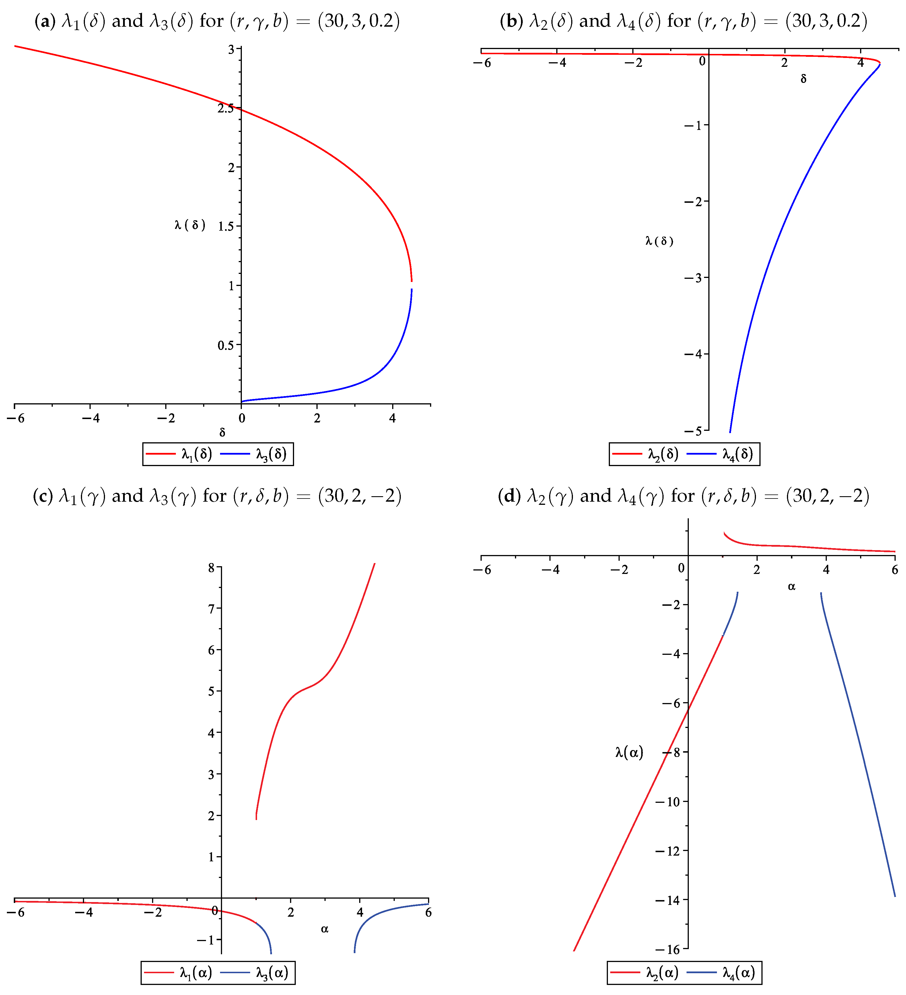
Note that, in Propositions 3 and 4, the eigenvalues of the Jacobian of $T_b$ on the nontrivial fixed points are written as functions of Lambert W functions. Figure 4 illustrates the variation in these eigenvalues according to the variation in the parameter $\delta$ (see Figure 4a,b), and according to the variation in the parameter $\gamma$ (see Figure 4c,d).

We now have the conditions to use Lemma 1 to obtain the nature and stability of the nontrivial fixed points $(x_i^{*},y_i^{*})$ of $T_b$, with $i=1,2,3,4$, obtained in Propositions 1 and 2. Note that whether the Allee effect parameter is odd or even, i.e., $\gamma =2n+1$ or $\gamma =2n$, the roots of the characteristic polynomial of the Jacobian of $T_b$, on these fixed points, are given by the following equation,

$${\lambda }^2-(1-b)(\gamma -\delta x_i^{*})\lambda -b=0.$$

Therefore, the next result is valid for both $\gamma$ odd and even. Note also that, from Corollary 1, we may assume $b\ne 1$.

Lemma 3.

Let $T_b:{\mathbb{R}}^2\to {\mathbb{R}}^2$ be the 2D γ-Ricker diffeomorphism defined by Equation (4). In the $(X^{*},{\Sigma }_b)$ space, for $\gamma \in \mathbb{N}\setminus \left\{1\right\}$, if $1-\gamma +\delta x_i^{*}>0$, then the fixed points $(x_i^{*},y_i^{*})$, with $i=1,2,3,4$, given by Equations (16)–(21) and (25)–(27), are classified as follows:

(i) 

a repeller point if, and only if, $1+\gamma -\delta x_i^{*}>0$ and $b<-1$;

(ii) 

a saddle point if, and only if, $1+\gamma -\delta x_i^{*}<0$;

(iii) 

an asymptotically stable point if, and only if, $1+\gamma -\delta x_i^{*}>0$ and $b>-1$;

(iv) 

a non-hyperbolic point if, and only if,

(a) 

$\gamma =-1+\delta x_i^{*}$ and $b\ne -2,0$;

(b) 

${(\gamma -\delta x_i^{*})}^2<1$ and $b=-1$.

Proof. 

The characteristic polynomial of the Jacobian matrix of $T_b$, on the fixed points $(x_i^{*},y_i^{*})$, with $i=1,2,3,4$, is $P\left(\lambda \right)={\lambda }^2-(1-b)(\gamma -\delta x_i^{*})\lambda -b$, where each $x_i^{*}$ is given by Equations (16)–(21) and Equations (25)–(27), respectively.

Note that the condition $P\left(1\right)>0$, mentioned in Lemma 1, is equivalent to writing,

$$1-(1-b)(\gamma -\delta x_i^{*})-b>0\iff (1-b)(1-\gamma +\delta x_i^{*})>0\iff 1-\gamma +\delta x_i^{*}>0.$$

The last equivalence is valid because as $\left|b\right|\le 1$ by the definition of ${\Sigma }_b$ in Equation (3) and we are considering the nontrivial fixed points of $T_b$, then $b\ne 1$. Thus, we conclude that $1-b>0$.

To prove item (i), each fixed point $(x_i^{*},y_i^{*})$, with $i=1,2,3,4$, is a repeller point if, and only if, the corresponding eigenvalues verify $|{\lambda }_1|>1$ and $|{\lambda }_2|>1.$ Considering Lemma 1, it follows that $|{\lambda }_j|>1$, for $j=1,2$, if, and only if, $P(-1)>0$ and $-b>1$. These conditions are equivalent to,

$$1+(1-b)(\gamma -\delta x_i^{*})-b>0\wedge b<-1$$

$$\iff (1-b)(1+\gamma -\delta x_i^{*})>0\wedge b<-1\iff 1+\gamma -\delta x_i^{*}>0\wedge b<-1.$$

This proves item (i).

The fixed point $(x_i^{*},y_i^{*})$, with $i=1,2,3,4$, is a saddle point if, and only if, $|{\lambda }_1|<1$ and $|{\lambda }_2|>1$ or $|{\lambda }_1|>1$ and $|{\lambda }_2|<1.$ Using Lemma 1, it follows that this happens if, and only if, $P(-1)<0,$ that is

$$(1-b)(1+\gamma -\delta x_i^{*})<0\iff 1+\gamma -\delta x_i^{*}<0.$$

So, the result of item (ii) follows.

The fixed point $(x_i^{*},y_i^{*})$, with $i=1,2,3,4$, is asymptotically stable if, and only if, $|{\lambda }_1|<1$ and $|{\lambda }_2|<1.$ It follows from Lemma 1 that $|{\lambda }_j|<1$, for $j=1,2$, if, and only if, $P(-1)>0$ and $-b<1$. This is equivalent to

$$(1-b)(1+\gamma -\delta x_i^{*})>0\wedge b>-1\iff 1+\gamma -\delta x_i^{*}>0\wedge b>-1.$$

Thus, we obtain the desired result of item (iii).

To prove item (iv), we have to consider two cases. The case ${\lambda }_1=-1$ and $|{\lambda }_2|\ne 1$ corresponds to a non-hyperbolic fixed point, where the eigenvalues are real. In this case, from Lemma 1, we have $P(-1)=0$ and $-b\ne 0,2.$ This is equivalent to,

$$(1-b)(1+\gamma -\delta x_i^{*})=0\wedge b\ne -2,0\iff \gamma =-1+\delta x_i^{*}\wedge b\ne -2,0.$$

This proves subitem $\left(a\right)$ of (iv). The second case, a non-hyperbolic fixed point where the eigenvalues ${\lambda }_1$ and ${\lambda }_2$ are complex numbers, with $|{\lambda }_1|=|{\lambda }_2|=1$, is verified if, and only if,

$${(1-b)}^2{(\gamma -\delta x_i^{*})}^2+4b<0\wedge -b=1\iff {(\gamma -\delta x_i^{*})}^2<1\wedge b=-1.$$

This proves subitem $\left(b\right)$ of (iv) and completes the proof. □

Note that the results established in Lemma 3 (i) and (iii) justify the definition of the embedding parameter $\left|b\right|\le 1$, as stated in the definition of ${\Sigma }_b$, given by Equation (3).

Given the complexity of the eigenvalues of the Jacobian of $T_b$ on the nontrivial fixed points, written in Propositions 3 and 4 as transcendental functions defined by Lambert W functions, and the respective classification established in Lemma 3, only the study of the bifurcations structure of $T_b$, presented in the next section, will provide a better understanding of its nonlinear dynamics.

4. Bifurcation Structures of the 2D $\mathbf{\gamma }$-Ricker Diffeomorphism ${\mathbf{T}}_{\mathbf{b}}$

This section is devoted to the study of the bifurcation structures of the 2D $\gamma$-Ricker diffeomorphism $T_b$. In view of the complexity of the fixed point expressions of $T_b$, given by Propositions 1 and 2, which correspond to transcendental functions defined by Lambert W functions, and in order to analyze the bifurcation structures of $T_b$, we consider the notion of contour lines in a parameter space. From now on, let $X^{*}=(x^{*},y^{*})$ be one of the k points of a cycle of order $k\in \mathbb{N}$, with $T_b(x,y)=(f_1,f_2)(x,y)$, given by Equation (4), and $T_b^k(x,y)=\left(f_1^{\left(k\right)},f_2^{\left(k\right)}\right)(x,y)$ be the k-iterated function from $T_b$. Consider the following expressions defined as follows,

$$N=\frac{\partial f_1^{\left(k\right)}}{\partial x}+\frac{\partial f_2^{\left(k\right)}}{\partial y}$$

(39)

and

$$D=\frac{\partial f_1^{\left(k\right)}}{\partial x}\frac{\partial f_2^{\left(k\right)}}{\partial y}-\frac{\partial f_1^{\left(k\right)}}{\partial y}\frac{\partial f_2^{\left(k\right)}}{\partial x}+1,$$

(40)

where N is the trace and $J=D-1$ is the determinant of the Jacobian matrix of $T_b^k\left(X^{*}\right)$, i.e., $J=\det \left(J\left(T_b^k\left(X^{*}\right)\right)\right)$, respectively. The real number $\sigma$ such that $D\sigma -N=0$ is called the reduced multiplier of the considered k-cycle. Note that the determinant of the Jacobian matrix of $T_b$ is $J=\det \left(J\left(T_b(x,y)\right)\right)=-b$.

Definition 1.

Let $T_b:{\mathbb{R}}^2\to {\mathbb{R}}^2$ be the 2D γ-Ricker diffeomorphism, defined by Equation (4), and $X^{*}=(x^{*},y^{*})$. In the $(X^{*},{\Sigma }_b)$ space, a contour line σ related to a k-cycle of $T_b$ is a curve which satisfies the following equations:

$$\left\{\begin{array}{c}{T}_b^k\left(X^{*}\right)-X^{*}=0\hfill \\ \\ D\left(X^{*}\right)\sigma -N\left(X^{*}\right)=0\hfill \end{array}\right.,$$

(41)

for a fixed value of $\sigma \in \mathbb{R}$ and $k\in \mathbb{N}$.

The notions of reduced multiplier, contour line and some properties concerning them are given in [28,29] (see also [11,12]). Note that a fixed point is also denoted by $(1;l)$-cycle, where $l\in \mathbb{N}$ is an index characterising the cycle and exchange order of the cycle points by successive applications of $T_b$. Generally, a k-cycle is designated by $(k;l)$ (see [5]).

In the following results, we establish the existence of the fixed points of $T_b$ on the corresponding contour lines $\sigma$.

Proposition 5.

Let $T_b:{\mathbb{R}}^2\to {\mathbb{R}}^2$ be the 2D γ-Ricker diffeomorphism, defined by Equation (4), and $X^{*}=(x^{*},y^{*})$. In the $(X^{*},{\Sigma }_b)$ space, with $b\ne 1$, the following properties hold true:

(i) 

for $b=1$, the fixed point $(x_0^{*},y_0^{*})=(0,0)$ exists on the contour line

$$\sigma ={\eta }_1\left(x_0^{*};r,\gamma ,\delta ,b\right)=0;$$

(ii) 

for $b\ne 1$, the fixed points $(x^{*},y^{*})=\left(\frac{\gamma -\sigma }{\delta },b\frac{\gamma -\sigma }{\delta }\right)$ exist on the contour lines

$$\sigma ={\eta }_2\left(x^{*};r,\gamma ,\delta ,b\right)=\frac{r\gamma {\left(x^{*}\right)}^{\gamma -1}{e}^{-\delta x^{*}}-\delta (1-b)x^{*}}{1-b}.$$

(42)

Proof. 

The proof of the previous results follows directly from Definition 1; considering $k=1$, it follows,

$$\left\{\begin{array}{c}{f}_1(x^{*},y^{*};r,\gamma ,\delta ,b)-x^{*}=0\hfill \\ \\ f_2(x^{*},y^{*};r,\gamma ,\delta ,b)-y^{*}=0\hfill \\ \\ D(x^{*},y^{*})\sigma -N(x^{*},y^{*})=0\hfill \end{array}\right.\iff \left\{\begin{array}{c}r{\left(x^{*}\right)}^{\gamma }{e}^{-\delta x^{*}}+b{x}^{*}=x^{*}\hfill \\ \\ b{x}^{*}=y^{*}\hfill \\ \\ \frac{\partial f_1}{\partial x}\left(x^{*}\right)=\sigma (1-b),\mathrm{for}{x}^{*}\ne 0\hfill \end{array}\right..$$

(43)

We remark that the equation $r{\left(x^{*}\right)}^{\gamma }{e}^{-\delta x^{*}}+b{x}^{*}=x^{*}$ is given by Equation (6). From the analysis of the $\gamma$-Ricker diffeomorphism $T_b$, the previous system can be written in the following equivalent form:

$$\left\{\begin{array}{c}\left(x_0^{*},y_0^{*}\right)=(0,0),\sigma =0,\mathrm{for}b=1\hfill \\ \\ \left(x^{*},y^{*}\right)=\left(\frac{\gamma -\sigma }{\delta },b\frac{\gamma -\sigma }{\delta }\right),\mathrm{for}b\ne 1\hfill \\ \\ \sigma =\frac{r\gamma {\left(x^{*}\right)}^{\gamma -1}{e}^{-\delta x^{*}}-\delta (1-b)x^{*}}{1-b}\hfill \end{array}\right..$$

(44)

So, the claims (i) and (ii) are proved. □

Remark 3.

The fixed points $(x^{*},y^{*})=\left(\frac{\gamma -\sigma }{\delta },b\frac{\gamma -\sigma }{\delta }\right)$, for $b\ne 1$, are the fixed points where the fold bifurcations occurs. So, the fixed points defined by Propositions 1 and 2 are the fixed points that are born from this bifurcation, according to the variation in the parameters stipulated in these results. In the particular case $b=1$, note that from Corollary 1, the fixed point $(x_0^{*},y_0^{*})=(0,0)$ corresponds to a Lyapunov critical case, i.e., ${\lambda }_1=-{\lambda }_2=1$, and exists on the contour line $\sigma =0$. On the other hand, considering $b\to 1^{-}$ in Equation (42), we obtain $r\to 0$, independent of the value of σ.

From this, the set defined by,

$$\Gamma =\left\{(r,\gamma ,\delta ,b)\in {\Sigma }_b:b=\omega (r,\gamma ,\delta )=1\right\}$$

(45)

is a singular set. Figure 5 and Figure 7 illustrate this remark.

Our next focus is the study of the bifurcation structures of $T_b$ in the parameter plane $(b,r)$, denoted by ${\Delta }_{b,r}$, for the Allee effect parameter $\gamma$ odd or even, and considering the parameter $\delta$ constant.

4.1. Case I: Parameter Plane ${\Delta }_{b,r}$, for $\gamma =2n+1$

The following proposition establishes a linear dependence between the fold and flip bifurcation curves of $T_b$ and $T_0$, for the fixed points in the parameter plane ${\Delta }_{b,r}$, considering the Allee effect parameter $\gamma =2n+1$.

Remark 4.

From [28] and Definition 1, it is known that, for a k-cycle, a contour line $\sigma =1$ is a fold bifurcation curve, denoted by ${\Lambda }_{{\left(k\right)}_0}^l$, and a contour line $\sigma =-1$ is a flip bifurcation curve, denoted by ${\Lambda }_k^l$ (see also [11,12]).

Proposition 6.

Let $T_b:{\mathbb{R}}^2\to {\mathbb{R}}^2$ be the 2D γ-Ricker diffeomorphism, defined by Equation (4), and $X^{*}=(x^{*},y^{*})$. In the $(X^{*},{\Sigma }_b)$ space, where $(x^{*},y^{*})$ and $\sigma ={\eta }_2\left(x^{*};r,\gamma ,\delta ,b\right)$ are defined as in Proposition 5 (ii), with $b\ne 1$, the following properties hold true:

(i) 

if $\gamma =2n+1$, then the fold or saddle-node bifurcation relative to the fixed points of $T_b$ in the parameter plane ${\Delta }_{b,r}$ is given by,

$$r={\phi }_1\left(x^{*},\sigma ;\gamma ,\delta ,b\right)={\phi }_1\left(x^{*},1;2n+1,\delta ,b\right)=(1-b){\left(\frac{\delta }{2n}\right)}^{2n}{e}^{2n},$$

(46)

with $(x^{*},y^{*})=\left(\frac{2n}{\delta },b{x}^{*}\right)$, for $\delta ={\delta }_0$ constant;

(ii) 

if $\gamma =2n+1$, then the flip or period-doubling bifurcation relative to the fixed points of $T_b$ in the parameter plane ${\Delta }_{b,r}$ is given by,

$$r={\psi }_1\left(x^{*},\sigma ;\gamma ,\delta ,b\right)={\psi }_1\left(x^{*},-1;2n+1,\delta ,b\right)=(1-b){\left(\frac{\delta }{2(n+1)}\right)}^{2n}{e}^{2(n+1)},$$

(47)

with $(x^{*},y^{*})=\left(\frac{2(n+1)}{\delta },b{x}^{*}\right)$, for $\delta ={\delta }_0$ constant.

Proof. 

Considering Equations (4), (39) and (40), Definition 1, Proposition 5 and Remark 4, we can establish that the fold or saddle-node bifurcation relative to the fixed points $(k=1)$ of $T_b$ in the parameter plane ${\Delta }_{b,r}$, with $b\ne 1$, $\gamma =2n+1$ and $\delta ={\delta }_0$ constant, satisfies the following equations,

$$\left\{\begin{array}{c}{T}_b(x^{*},y^{*})=(x^{*},y^{*})\hfill \\ \\ D(x^{*},y^{*})=N(x^{*},y^{*})=\frac{\partial T_0}{\partial x}\left(x^{*}\right)=1-b\hfill \end{array}\right.\iff \left\{\begin{array}{c}(x^{*},y^{*})=\left(\frac{2n}{\delta },b\frac{2n}{\delta }\right)\hfill \\ \\ r=(1-b){\left(\frac{\delta }{2n}\right)}^{2n}{e}^{2n}\hfill \end{array}\right..$$

(48)

Thus, we obtain the desired result of item (i).

In a similar way, claim (ii) is obtained by applying Definition 1, Proposition 5 and Remark 4, for $\sigma =-1$ and $k=1$. Consequently, the flip bifurcation relative to the $(1;l)$-cycle of $T_b$ satisfies the following equations,

$$\left\{\begin{array}{c}{T}_b(x^{*},y^{*})=(x^{*},y^{*})\hfill \\ \\ D(x^{*},y^{*})=-N(x^{*},y^{*})=\frac{\partial T_0}{\partial x}\left(x^{*}\right)=b-1\hfill \end{array}\right.\iff \left\{\begin{array}{c}(x^{*},y^{*})=\left(\frac{2(n+1)}{\delta },b\frac{2(n+1)}{\delta }\right)\hfill \\ \\ r=(1-b){\left(\frac{\delta }{2(n+1)}\right)}^{2n}{e}^{2(n+1)}\hfill \end{array}\right..$$

(49)

Therefore, we obtain the result of claim (ii). □

Equations (48) and (49) give us the explicit equations of the fold and flip bifurcation curves relative to the fixed points of $T_b$, in the parameter plane ${\Delta }_{b,r}$. In Figure 5 are plotted the fold bifurcation curve ${\Lambda }_{{\left(1\right)}_0}$ and the flip bifurcation curve ${\Lambda }_1$, given by Equations (48) and (49), respectively, for $\gamma =3$ and $\delta =2$. Note that the fold and flip bifurcation curves defined by $r={\phi }_1\left(x^{*},1;2n+1,\delta ,b\right)$ and $r={\psi }_1\left(x^{*},-1;2n+1,\delta ,b\right)$ are only defined in the semi-plane $r>0$ of the parameter plane ${\Delta }_{b,r}$. This behaviour is a consequence of Property 3 because if $r<0$, then $W\left(A_i(r,\gamma ,\delta ,b)\right)\in \mathbb{C}$. This means that $T_b$ has no real fixed points for $r<0$ and consequently there are no bifurcation curves for this cycle. Thus, in the semi-plane $r>0$ exists a bifurcation cascade of $T_b$, which occurs in an interval of existence of an attractive limit set at a finite distance, which is defined by,

$${\Omega }_1=[r_{{\left(1\right)}_0},r_1^{*}],\forall (r,\gamma ,\delta ,b)\in {\Sigma }_b,\mathrm{with}r>0\mathrm{and}\gamma =2n+1.$$

(50)

This set is called a “principal” box or first box of the first kind ${\Omega }_1$, where occur all the possible bifurcations of $T_b$ in ${\Sigma }_b$. The box ${\Omega }_1$ starts at $r_{{\left(1\right)}_0}$, given by Equation (48), when the attracting fixed point $(x^{*},y^{*})$ appears and the fold bifurcation of $T_b$ occurs at $k=1$. The end of this box is verified at $r_1^{*}$, when the first homoclinic bifurcation of the fixed points appears (see [5]). On one hand, an increase in the parameter r through the interval ${\Omega }_1$ generates the set of all bifurcations of $T_b$ in the ${\Delta }_{b,r}$ parameter plane, for $r>0$ (see Figure 5). We remark that we use the letters H and B to denote and differentiate the bifurcation curves in the semi-planes $r>0$ and $r<0$, respectively.

On the other hand, in the semi-plane $r<0$ of the parameter plane ${\Delta }_{b,r}$, for $b>0$, a bifurcation cascade of $T_b$ is detected for the second box ${\Omega }_2$ associated with a cycle of order $k=2$, defined by,

$${\Omega }_2=[r_{{\left(2\right)}_0},r_2^{*}],\forall (r,\gamma ,\delta ,b)\in {\Sigma }_b,\mathrm{with}r<0,b>0\mathrm{and}\gamma =2n+1,$$

(51)

where $r_{{\left(2\right)}_0}$ is given by Equation (41), for $k=2$ and $\sigma =1$, and $r_2^{*}$ is given by the parameter value for which the first homoclinic bifurcation of the cycle of order $k=2$ appears (see [5]). In Figure 5, we can see the fold bifurcation curve${ }^B{\Lambda }_{{\left(2\right)}_0}$ of the cycle $k=2$, for which the box ${\Omega }_2$ starts and then it follows the period doubling region. Still, on the semi-plane $r<0$, with $b<0$, we see the existence of a cusp point $C_3$ related to the cycle of order $k=3$, from which emerges a saddle area. The existence of this cusp point $C_3$ allows us to consider the emergence of a communication area, which will be centered on this fold codimension-2 singularity. A detailed description of a saddle communication area can be found in [4,28] and the references therein. This particular bifurcation structure develops into another independent box of those previously considered in Equations (50) and (51). In this case, we have a third box ${\Omega }_3$ associated with a cycle of order $k=3$, defined by,

$${\Omega }_3=[r_{{\left(3\right)}_0},r_3^{*}],\forall (r,\gamma ,\delta ,b)\in {\Sigma }_b,\mathrm{with}r<0,b<0\mathrm{and}\gamma =2n+1,$$

(52)

where $r_{{\left(3\right)}_0}$ is given by Equation (41), for $k=3$ and $\sigma =1$, and $r_3^{*}$ is given by the parameter value for which the first homoclinic bifurcation of this cycle of order $k=3$ appears, restricted to the parameter values considered.

In the following result is presented a property that characterizes the bifurcation structure of $T_b$ in the ${\Delta }_{b,r}$ parameter plane.

Property 7.

Let $T_b:{\mathbb{R}}^2\to {\mathbb{R}}^2$ be the 2D γ-Ricker diffeomorphism, defined by Equation (4). In the $(X^{*},{\Sigma }_b)$ space, if $\gamma =2n+1$ and $\delta ={\delta }_0$ constant, then, in the ${\Delta }_{b,r}$ parameter plane exists a flip codimension-2 bifurcation point relative to the fixed points of $T_b$ (parametric node) given by,

$$N_1={\Lambda }_{{\left(1\right)}_0}\cap {\Lambda }_1=\left\{(b,r)\in {\Delta }_{b,r}:b\to 1^{-},r\to 0^{+}\right\}.$$

Proof. 

From Proposition 6, in particular Equations (46) and (47), and concerning the ${\Delta }_{b,r}$ parameter plane, for $\gamma =2n+1$ and $\delta ={\delta }_0$ constant, if we consider the limit when $b\to 1^{-}$, then it follows,

$${\displaystyle \underset{b\to 1^{-}}{lim}{\phi }_1\left(x^{*},1;2n+1,\delta ,b\right)=\underset{b\to 1^{-}}{lim}{\psi }_1\left(x^{*},1;2n+1,\delta ,b\right)=0^{+}.}$$

Consequently, the point $N_1=(b\to 1^{-},r\to 0^{+})$ is a tangency of the fold and flip bifurcation curves ${\Lambda }_{{\left(1\right)}_0}$ and ${\Lambda }_1$ relative to the fixed points of $T_b$. From Corollary 1, considering $b=1$, the fixed point $(x_0^{*},y_0^{*})=(0,0)$ is unique and corresponds to a Lyapunov critical case, i.e., ${\lambda }_1=-{\lambda }_2=1$, independent of the $\sigma$ value (see also Remark 3). Thus, we obtain the desired result (see also Figure 5). □

Note that from Figure 5, on the singular set $\Gamma$, given by Equation (45), it is also verified that,

$$N_1={\Lambda }_{{\left(1\right)}_0}\cap {\Lambda }_1\cap { }^B{\Lambda }_{{\left(2\right)}_0},$$

where${ }^B{\Lambda }_{{\left(2\right)}_0}$ is the fold bifurcation curve relative to a cycle of order $k=2$.

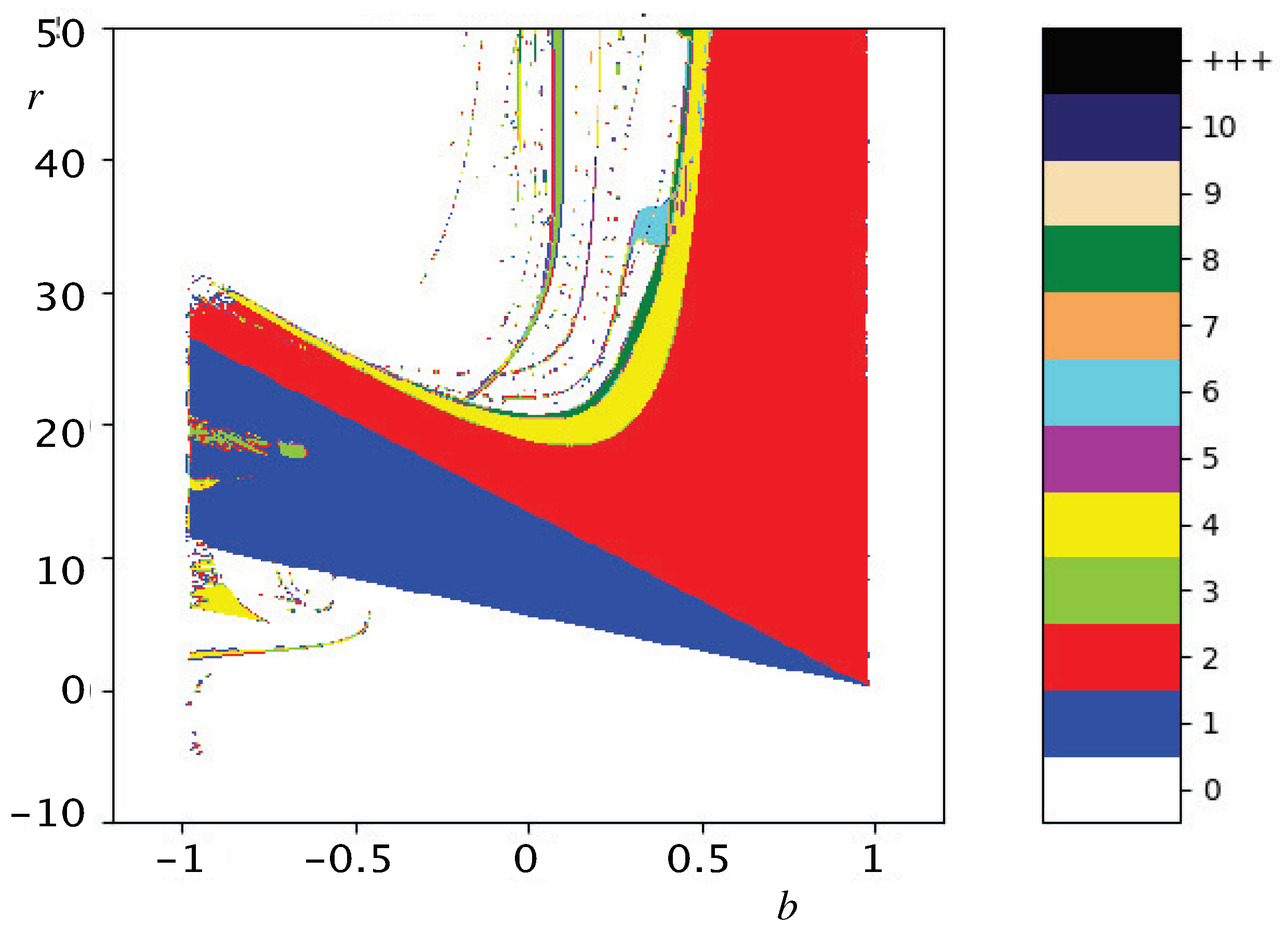
Figure 6 illustrates a bifurcation diagram of the 2D $\gamma$-Ricker diffeomorphism $T_b$ in the ${\Delta }_{b,r}$ parameter plane, at $\gamma =3$ and $\delta =2$. In the semi-plane $r>0$, the blue region is the stability region of the nonzero fixed points, given by Proposition 1. The red, yellow and green sequence regions correspond to the period doubling region (periods of order $k=2,4,8$, respectively), and then it follows the chaotic region. In the semi-plane $r<0$ and $b>0$, another period doubling cascade is visible, correspondent to the box ${\Omega }_2$, given by Equation (51). Finally, in the semi-plane $r<0$ and $b<0$, there is a slight configuration of the saddle communication area, which emerges from the cusp point $C_3$, as described above.

4.2. Case II: Parameter Plane ${\Delta }_{b,r}$, for $\gamma =2n$

In this section, we analyze the bifurcation structures of $T_b$ in the parameter plane ${\Delta }_{b,r}$, considering the Allee effect parameter $\gamma =2n$. The following results show the explicit equations for the fold and flip bifurcation curves, relative to the fixed points of $T_b$.

Proposition 7.

Let $T_b:{\mathbb{R}}^2\to {\mathbb{R}}^2$ be the 2D γ-Ricker diffeomorphism, defined by Equation (4), and $X^{*}=(x^{*},y^{*})$. In the $(X^{*},{\Sigma }_b)$ space, where $(x^{*},y^{*})$ and $\sigma ={\eta }_2\left(x^{*};r,\gamma ,\delta ,b\right)$ are defined as in Proposition 5 (ii), with $b\ne 1$, the following properties hold true:

(i) 

if $\gamma =2n$, then the fold or saddle-node bifurcation relative to the fixed points of $T_b$ in the parameter plane ${\Delta }_{b,r}$ is given by,

$$r={\phi }_2\left(x^{*},\sigma ;\gamma ,\delta ,b\right)={\phi }_2\left(x^{*},1;2n,\delta ,b\right)=(1-b){\left(\frac{\delta }{2n-1}\right)}^{2n-1}{e}^{2n-1},$$

(53)

with $(x^{*},y^{*})=\left(\frac{2n-1}{\delta },b{x}^{*}\right)$, for $\delta ={\delta }_0$ constant;

(ii) 

if $\gamma =2n$, then the flip or period-doubling bifurcation relative to the fixed points of $T_b$ in the parameter plane ${\Delta }_{b,r}$ is given by,

$$r={\psi }_2\left(x^{*},\sigma ;\gamma ,\delta ,b\right)={\psi }_2\left(x^{*},-1;2n,\delta ,b\right)=(1-b){\left(\frac{\delta }{2n+1}\right)}^{2n-1}{e}^{2n+1},$$

(54)

with $(x^{*},y^{*})=\left(\frac{2n+1}{\delta },b{x}^{*}\right)$, for $\delta ={\delta }_0$ constant.

The proof of the results of Proposition 7 is similar to the proof of Proposition 6, with the respective analysis of the case $\gamma =2n$.

In Figure 7 are plotted some bifurcation curves of the 2D $\gamma$-Ricker diffeomorphism $T_b$, for $\gamma =2$ and $\delta =2$. Similar to the results presented in Section 2.2, concerning the existence of nontrivial fixed points of $T_b$ for $\gamma =2n$ (see Remark 1), the bifurcation structure of $T_b$ in the ${\Delta }_{b,r}$ parameter plane will be analogous to the bifurcation structure of $T_b$, for $\gamma =2n+1$ and $x>0$. In fact, we can confirm this similarity between Figure 5 and Figure 7 by considering the semi-plane $r>0$. The fold and flip bifurcation curves plotted have the same meaning as described above. We remark that for $\gamma =2n$ there is only the bifurcation cascade associated with the box ${\Omega }_1$, given by Equation (50). The bifurcation diagram of the 2D $\gamma$-Ricker diffeomorphism $T_b$, with $\gamma =2$ and $\delta =2$, in the ${\Delta }_{b,r}$ parameter plane, is represented in Figure 8, which similarly behaves like the bifurcation diagram in Figure 6, for the semi-plane $r>0$.

5. Discussion and Conclusions

In this work, we introduced a new 2D $\gamma$-Ricker population model, defined using the diffeomorphism $T_b$, given by Equation (4). The aim of this two-dimensional model was to understand the nonlinear dynamics in 2D of the classic 1D $\gamma$-Ricker population model, through the embedding parameter b. The first imperative question we sought to answer was about the number of fixed points of $T_b$ and how to define them, since the expression for determining them is implicit. In this way, using Lambert W functions, it was possible to define the fixed points of $T_b$ as analytical solutions of these transcendental functions. Properties 3 and 4 establish conditions on the parameters space ${\Sigma }_b$ for which the Lambert W functions admit solutions or not. Consequently, in Propositions 1 and 2, the main results of this work, established in Theorem 1, on the maximum number of fixed points of $T_b$ have been proved. This study was analyzed taking into account the parity of the Allee effect parameter $\gamma$, which provides significant differences.

In order to clarify the nonlinear dynamics and bifurcation structures of the 2D $\gamma$-Ricker diffeomorphism $T_b$, an exhaustive study was carried out on the nature and stability of the fixed points of $T_b$. However, due to the complexity of defining the nontrivial fixed points of $T_b$ using Lambert W functions, this classification has become intricate and difficult, because the eigenvalues of $T_b$ are also defined through Lambert W functions, for the parameter $\gamma$ odd and even, according to the results proved in Propositions 3 and 4, and Lemma 3. Specifically, the trivial fixed point of $T_b$ is also recognised to have a significant role in this study, namely, in the particular cases $\gamma =1$ and $b=1$, as we discussed in the results presented in Lemma 2 and Corollary 1.

In the last phase of our work, we studied the bifurcation structures of the 2D $\gamma$-Ricker diffeomorphism $T_b$ in the parameter plane ${\Delta }_{b,r}$, considering again the parity of the Allee effect parameter $\gamma$. In order to complete this study, we have used the fold and flip bifurcation curves, which are defined as particular cases of contour lines related to cycles of order k of $T_b$. For the numerical cases analyzed, the stability domains of the different cycles of order $k=1,2,3,4,5,8$ were determined in the respective bifurcation diagrams. Thus, the analytical and numerical implementation of these two case studies sustained the theoretical results obtained in the previous sections, in particular, the differentiation between the behaviour of this 2D population model for the Allee effect parameter odd or even. Therefore, for this model, the performance of the parameter $\gamma$ is crucial.

This work has led us to some extremely important and complex questions for our future research. The main question concerns the analysis of the 2D $\gamma$-Ricker diffeomorphism $T_b$, considering the Allee effect parameter $\gamma \in {\mathbb{R}}^{+}$. In this way, we will have to characterise the phenomenon of the Allee effect for this 2D population growth model, establishing conditions for its existence, as well as justifying what the differentiating role of the Allee effect is in the bifurcation structures of $T_b$.