Developing and Evaluating the Operating Region of a Grid-Connected Current Source Inverter from Its Mathematical Model

Abstract

Grid-connected power inverters are indispensable in modern electrical systems, playing a pivotal role in enhancing the integration of renewable energies into power grids. Their significance, primarily when functioning as grid-forming inverters, extends to maintaining the grid’s inertia and strength—a distinct advancement over traditional grid-following operations. As grid-forming inverters, these devices emulate the characteristics of synchronous generators and can act as robust voltage sources, providing essential ancillary services. This behavior is particularly relevant when integrating energy storage systems on the converters’ direct current side. Among the various inverter topologies, the current source inverter (CSI) has emerged as a promising yet underexplored alternative for grid-forming applications. CSIs, when paired with their AC output filters, can effectively operate as voltage sources, utilizing control strategies that facilitate the integration of renewable energies into the electrical system. Their design inherently manages output current fluctuations, reducing the need for restrictive current limitations or additional protective measures. This paper examines the operational region of CSIs, obtained through detailed modeling, to explore their advantages, challenges, and potential for enhancing grid-connected systems. Analyzing the operating region from the converter model verifies the limits of where the converter can operate in a plane of active and reactive powers. For a small prototype model operating with 7 amperes in DC and 120 V in AC, it is possible to supply or absorb active power exceeding 1000 W and manage maximum reactive power values around 500 VAr, as determined by its operating region. Simulations also confirm that small changes in the control reference, as little as 5%, towards the region’s right limits cause significant oscillations in the dynamic control responses. This research aims to deepen our understanding of CSIs’ operational capabilities and highlight their unique benefits in advancing grid-connected systems and promoting the integration of renewable energy using this technology.

1. Introduction

Over the past few decades, the increasing integration of renewable energies into our power systems has posed challenges to both power quality and grid stability, while traditional grid-following inverters effectively channel power from renewable sources, they are not inherently designed to provide essential frequency or voltage support to the power grids [1]. This absence of voltage and frequency support becomes particularly evident when grid dynamics lead to deviations from nominal frequency and voltage values. Insights gained from microgrid research have unveiled various operational modes for grid-connected inverters. These modes have introduced specific terminologies for inverter operation within microgrids, including grid-following (GFL), grid-forming (GFM), and grid-supporting (GSP) inverters. In each operational mode, grid-connected inverters display behaviors as either voltage or current sources, as illustrated in Figure 1. The key differences between these operational modes lie in their control strategies. GFL inverters traditionally use maximum power point tracking (MPPT) techniques to consistently extract maximum power from renewable generation systems. They also employ phase-locked loop (PLL) algorithms to synchronize with the grid voltage. These synchronization algorithms can generally be used in GSP inverters as well. In contrast, most GFM inverters do not require PLLs, making them more robust in maintaining stable operation under normal grid conditions.

A GFL inverter maximizes power transfer from the DC side to the AC grid, consistently synchronizing with the frequency and voltage of the connected electrical grid. On the other hand, a GFM inverter demonstrates remarkable resilience by generating power even during grid disconnection or outages, supporting ‘black start’ scenarios [2,3]. This establishes the frequency and voltage of the microgrid if it operates in isolation from the primary grid, functioning as a reference for other connected converters. Additionally, it offers voltage and frequency support when integrated with the primary grid. Meanwhile, a GSP inverter aims to deliver power from its sources while enhancing grid stability. This can be achieved by providing targeted frequency support through its control mechanisms and converter, as depicted in Figure 1. Additionally, it can potentially offer voltage support. The GSP inverter can operate as a controlled current source, as shown in Figure 1, but it can also function as a voltage source [4]. To emphasize the different control strategies involved, Figure 1 illustrates only one option. For a more comprehensive understanding of these concepts, please refer to [5].

The predominant operation of grid-connected inverters as GFL inverters means that as the amount of renewable energy delivered through such inverters increases, the overall system inertia and the capability to handle frequency and voltage contingencies diminish [6]. However, recent studies have suggested that GFM inverters, which emulate the behavior of synchronous generators, could theoretically enable near-limitless integration of renewable energies into electric grids [7,8]. This advancement primarily leaves the challenge of renewable energy intermittency, a concern potentially mitigated by the augmented deployment of energy storage devices [9,10]. Presently, a variety of control strategies exist to achieve GFM inverters [11]. The droop control scheme stands as the most foundational and widely recognized method [12,13]. Moreover, direct power control has seen several years of application. Yet, numerous other control schemes have emerged recently [14].

While the specific control scheme may vary to realize a GFM inverter, it is important to note that this mode can be implemented across virtually any inverter topology, as a GFM inverter is essentially an operational mode of a grid-connected inverter. Among the topologies, the VSI remains the most practical and recognized, within which most GFM strategies have been tested. However, studying the CSI for GFM is particularly attractive in this context [15]. If the perspective is expanded to grid-connected operation, it could be said that in recent years, there has been increasing interest in grid-connected CSI for enhanced grid operation [16,17,18,19]. In this regard, a comprehensive review of the state of the art is provided in Chapter 2 of this article.

This article presents a novel approach by proposing and exploring the operating regions of grid-forming inverters implemented with the CSI topology enhanced with a CLC (Capacitive-Inductive-Capacitive) filter, which is not addressed in the existing literature. Additionally, the article presents simulations to demonstrate the operation and dynamics within the working zone of the converter. The document is organized as follows: Section 1 contextualizes how power inverters can operate when connected to microgrids and electrical networks. Section 2 briefly compares the VSI and CSI topologies, delving into a detailed review of the state of the art regarding grid-connected CSIs and introducing the operation of the CSI as a grid-forming inverter. Section 3 provides a complete modeling of the grid-connected CSI, covering both dynamic performance and steady-state behavior. Section 4 explains the process of obtaining and analyzing the operating region of the current source converter. Section 5 corroborates the determination of the operating region through simulations at various operating points. Section 6 discusses and comments on the results, and Section 7 draws the document’s conclusions.

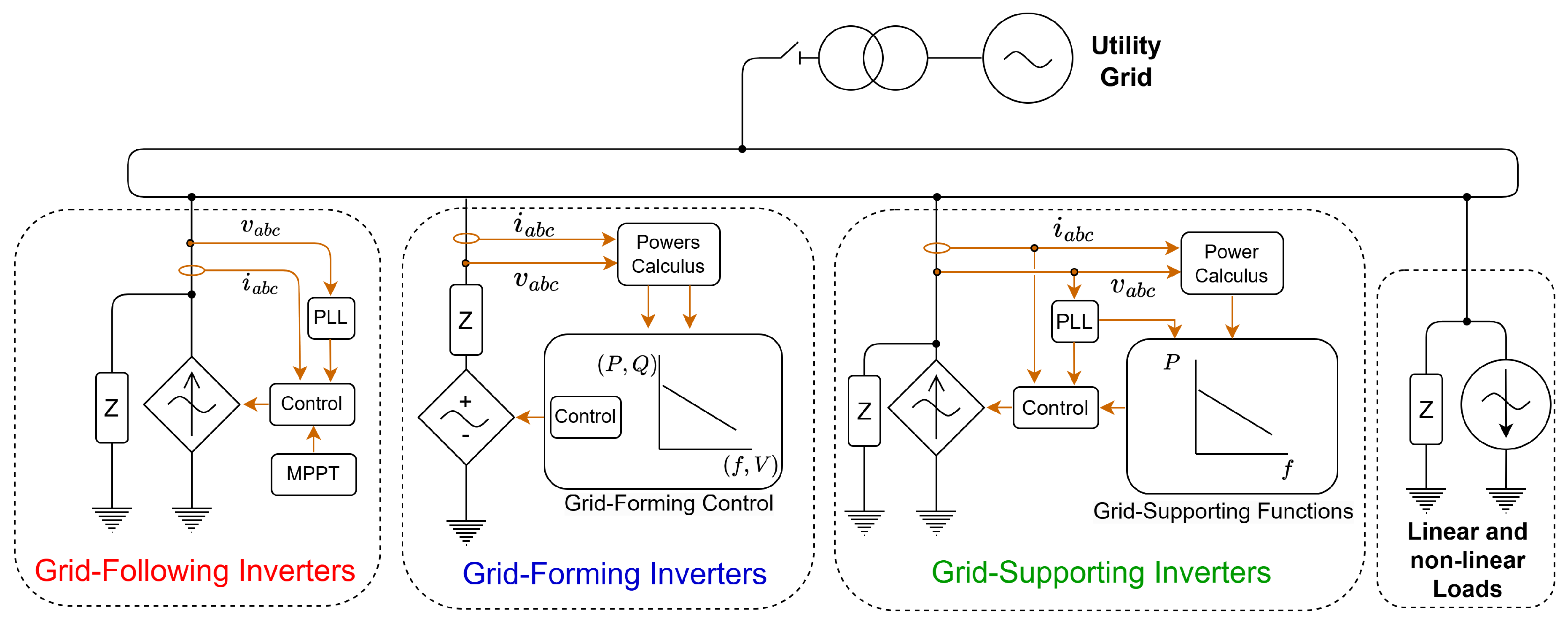
2. Grid-Forming Inverters Topologies and Control Schemes

2.1. A Brief Comparison between VSI and CSI Topologies

From a topological perspective, the conventional approach to implementing a grid-forming inverter considers a voltage source inverter (VSI). Typically, the VSI incorporates an LCL filter at its AC output before serving local loads or interfacing with the primary grid, as seen in [20,21,22]. Alternatively, the current source inverter (CSI) has been tested as a grid-connected inverter and can be a topological option for grid-forming inverter operation [15,23,24]. Although its potential in grid-forming applications remains largely untapped, interest in CSI topology has persisted over the years for various other applications [25,26,27]. When functioning as a grid-forming inverter, the CSI can integrate a CLC (Capacitive-Inductive-Capacitive) filter on its AC output. This filter helps to improve the voltage and power quality provided by the inverter. Similar to its VSI counterpart, it can operate in connected and isolated modes, as depicted in Figure 2. Historically, the CSI has often been overshadowed by the VSI due to perceived technological constraints [28]. The DC-link of the CSI contains a DC current source demanding management, complemented by a series choke inductor.

The merits of the VSI in comparison to the CSI are both evident and extensively documented [28,29,30,31]. A concise comparison of the strengths and limitations of both topologies is presented in

Table 1. A brief comparison of advantages and disadvantages in classic VSI and CSI topologies.

Topology	Advantages	Disadvantages
VSI	Efficient dc filter with very low energy losses. Low weight of filter (storage element). It can be switched with frequencies (10 kHz∼20 kHz). It is a more well-known technology.	Highly vulnerable to damage from short circuits. It is necessary to regulate and/or limit the output current. Observed reliability falls short of aspirational standards Parallel operation is a challenge
CSI	Natural short-circuit protection It is easier to operate several in parallel on AC sides. Very high reliability can be achieved	It is difficult to achieve high efficiency. More complex modulation and control. There are losses even in a zero-switching state. The volume and weight of the DC filter are evident.

. Among the notable benefits of the VSI is the relative ease with which a converter can be implemented using this technology. The contemporary market even offers ready-to-use power modules. The efficiency of VSIs is further accentuated by incorporating DC capacitors on the DC side, which serve as filters. The maturation of capacitor technology ensures both quality and longevity for these components.

Additionally, the reduction in the equivalent series resistance of capacitors and the potential associated loss is evidence of ongoing advancements in this domain. Conversely, DC links in the CSI utilize choke inductors. Several new CSI topologies are emerging, aiming to improve or modify the design on the DC side of these converters [32,33,34]. Experts in power electronics opine that strides in superconductor development are imperative for choke inductors to attain a technological maturity akin to capacitors [35]. This progression is crucial to mitigating losses associated with filtering DC ripple in CSIs [36,37].

However, the CSI finds niche applications where DC-controlled current is crucial, particularly in systems that demand high reliability. As a topology, it is more reliable than the VSI [38,39]. It is anticipated that future advancements in superconductor technology will further enable the proliferation of CSIs across various applications, leveraging its inherent short-circuit protection [35,40].

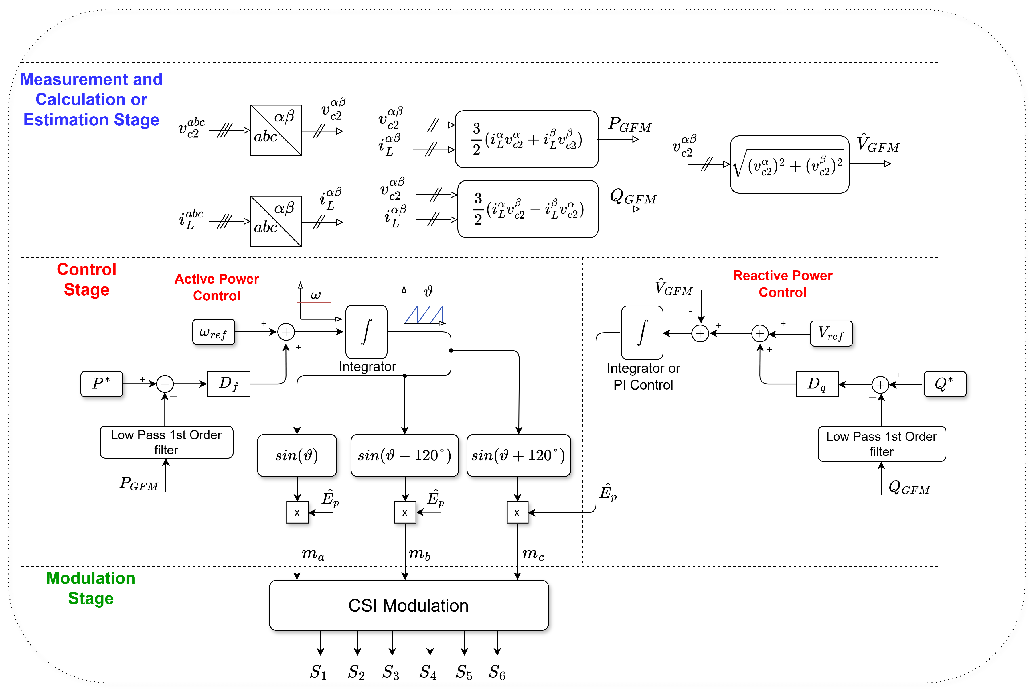
2.2. Grid-Forming Control Scheme

In recent years, significant attention has been directed toward GFM inverters, as they hold the potential to facilitate the widespread integration of renewable energy into our electrical grids. These GFM inverters are attainable through advanced control strategies, while the foundational and well-established droop control strategy remains popular for achieving GFM operation, numerous alternative approaches have emerged in recent research. These alternatives empower the inverter to function as a voltage source and provide valuable grid services, including black start capability and inertia support, among other capabilities [41].

A notable control scheme that enables a CSI to function effectively as a GFM inverter is the well-known droop control strategy. Implementing this strategy in the CSI, precisely as depicted in Figure 3, eliminates the need for a traditional inner current control loop—typically used in VSI systems—thanks to the CSI’s inherent ability to regulate current both at the DC side and at the inverter’s output.

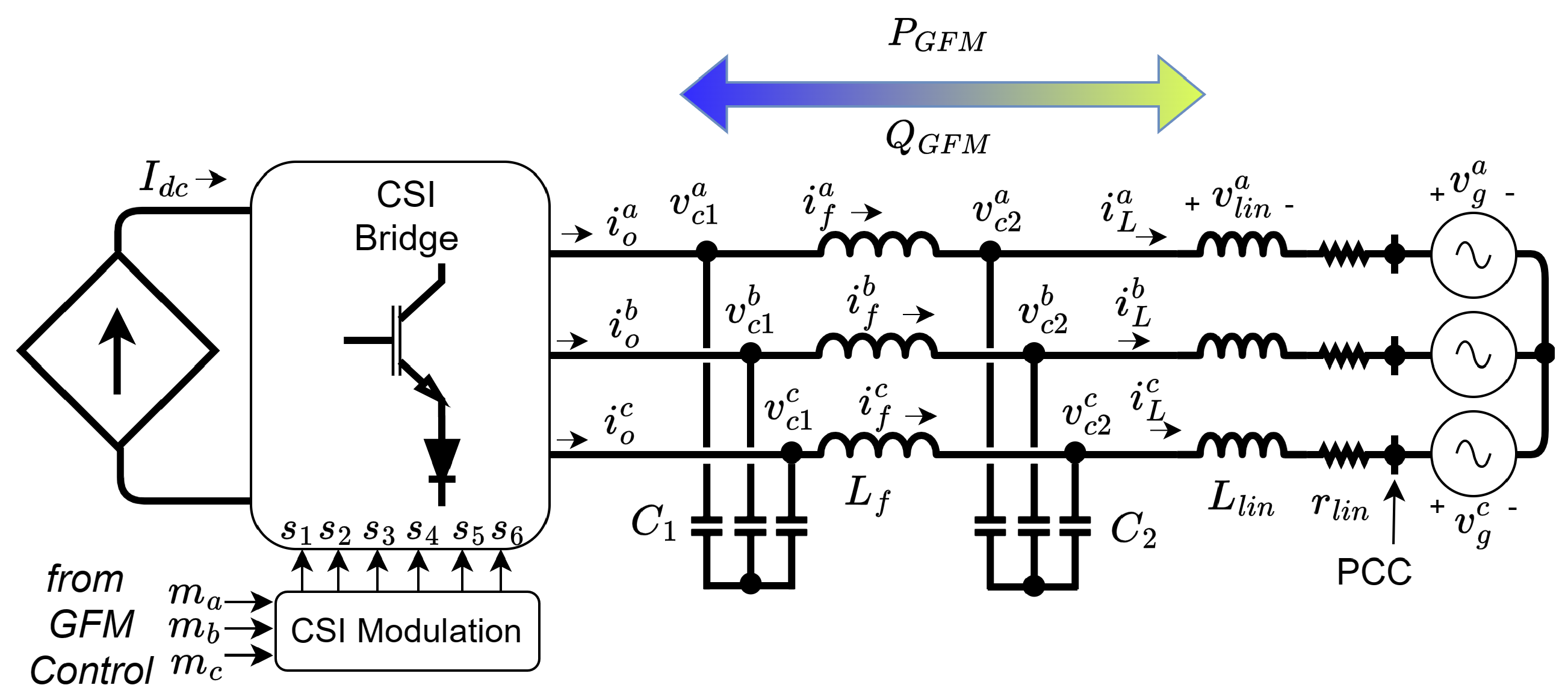
3. Modeling of a Grid-Connected CSI

3.1. Dynamic Behavior Modeling

A GFM inverter implemented with a CSI, through a droop control scheme as shown in Figure 3, will seek to impose its voltages $v_{c2}^a$, $v_{c2}^b$, and $v_{c2}^c$ at the terminals at the output of its CLC filter. If this inverter operates in a microgrid connected to the main grid, then the currents $i_L^a$, $i_L^b$, and $i_L^c$ supplied or absorbed by the CSI will be managed by the inverter’s control scheme (contributing or absorbing active powers $P_{GFM}$ and/or reactive powers $Q_{GFM}$). In the case that the microgrid is isolated, these same currents (and powers) will be demanded by the microgrid, altering the voltage and frequency of the inverter according to the predefined curves in the same control scheme [42]. To determine how much power ($P_{GFM}$ and $Q_{GFM}$) the inverter can contribute or absorb through its operating region, it will be necessary to know its model, whether the inverter operates in a microgrid connected to the main grid or in isolation. For this purpose, a description can be made using the variables observed in Figure 4. Therefore, the three voltages in the capacitances with a value of $C_1$ can be expressed as follows:

$$\begin{array}{c}\hfill \frac{d{v}_{c1}^a}{dt}=\frac{1}{C_1}(i_o^a-i_f^a)\\ \hfill \frac{d{v}_{c1}^b}{dt}=\frac{1}{C_1}(i_o^b-i_f^b)\\ \hfill \frac{d{v}_{c1}^c}{dt}=\frac{1}{C_1}(i_o^c-i_f^c)\end{array}\}.$$

(1)

If a compact notation is adopted, it is possible to present the three equations of the set expressed in (1) as a single equation as follows:

$$\frac{d{\mathbf{v}}_{\mathbf{c}\mathbf{1}}^{\mathbf{abc}}}{dt}=\frac{1}{C_1}({\mathbf{i}}_{\mathbf{o}}^{\mathbf{abc}}-{\mathbf{i}}_{\mathbf{f}}^{\mathbf{abc}}),$$

(2)

where

$${\mathbf{i}}_{\mathbf{o}}^{\mathbf{abc}}={\left[\begin{array}{ccc}{i}_o^a& i_o^b& i_o^c\end{array}\right]}^T,$$

(3)

corresponds to a three-phase array consisting of the output currents $i_o^a$, $i_o^b$ and $i_o^c$, whereas

$${\mathbf{i}}_{\mathbf{f}}^{\mathbf{abc}}={\left[\begin{array}{ccc}{i}_f^a& i_f^b& i_f^c\end{array}\right]}^T,$$

(4)

is an array composed of the currents passing through the filter inductances, specifically $i_f^a$, $i_f^b$, and $i_f^c$. Moreover, it is required that

$$\frac{d{\mathbf{v}}_{\mathbf{c}\mathbf{1}}^{\mathbf{abc}}}{dt}={\left[\begin{array}{ccc}\frac{d{v}_{c1}^a}{dt}& \frac{d{v}_{c1}^b}{dt}& \frac{d{v}_{c1}^c}{dt}\end{array}\right]}^T,$$

(5)

which is the array of the derivatives of the voltages $v_{c1}^a$, $v_{c1}^b$ and $v_{c1}^c$, which are the voltages across the first capacitor bank.

Taking into account the voltages within the CLC filter, it is possible to present the state equation of the currents in the filter inductor (in a compact notation) as

$$\frac{d{\mathbf{i}}_{\mathbf{f}}^{\mathbf{abc}}}{dt}=\frac{1}{L_f}({\mathbf{v}}_{\mathbf{c}\mathbf{1}}^{\mathbf{abc}}-{\mathbf{v}}_{\mathbf{c}\mathbf{2}}^{\mathbf{abc}}),$$

(6)

where ${\mathbf{v}}_{\mathbf{c}\mathbf{1}}^{\mathbf{abc}}$ contains the voltages $v_{c1}^a$, $v_{c1}^b$, and $v_{c1}^c$, while ${\mathbf{v}}_{\mathbf{c}\mathbf{2}}^{\mathbf{abc}}$ contains the voltages $v_{c2}^a$, $v_{c2}^b$, and $v_{c2}^c$. Similarly, the behavior of the voltages across the capacitor $C_2$ can be expressed as:

$$\frac{d{\mathbf{v}}_{\mathbf{c}\mathbf{2}}^{\mathbf{abc}}}{dt}=\frac{1}{C_2}({\mathbf{i}}_{\mathbf{f}}^{\mathbf{abc}}-{\mathbf{i}}_{\mathbf{L}}^{\mathbf{abc}}),$$

(7)

where the array of currents ${\mathbf{i}}_{\mathbf{L}}^{\mathbf{abc}}$ contains the load currents of the inverter $i_L^a$, $i_L^b$, and $i_L^c$, contributed to or absorbed from the PCC (Point of Common Coupling).

Given the converter’s connection to the Point of Common Coupling (PCC) through a line characterized by a small inductance ($L_{lin}$) and minimal resistance ($r_{lin}$), forming the line impedance and excluding the consideration of a local load for this context, as can be seen in Figure 4, the following equations are applicable within the ABC coordinate system:

$$\frac{d{\mathbf{i}}_{\mathbf{L}}^{\mathbf{abc}}}{dt}=\frac{1}{L_{lin}}({\mathbf{v}}_{\mathbf{c}\mathbf{2}}^{\mathbf{abc}}-r_{lin}{\mathbf{i}}_{\mathbf{L}}^{\mathbf{abc}}-{\mathbf{v}}_{\mathbf{g}}^{\mathbf{abc}}),$$

(8)

where $v_g^{abc}$ corresponds to the grid voltages to which the inverter is connected.

In the case of a perfectly balanced system, Equations (2), (6), (7), and (8) can be transformed into $dq$ axes using compact notation. These four equations can now be expressed as:

$$\begin{array}{c}\frac{d{\mathbf{v}}_{\mathbf{c}\mathbf{1}}^{\mathbf{dq}}}{dt}=-\mathbf{W}{\mathbf{v}}_{\mathbf{c}\mathbf{1}}^{\mathbf{dq}}+\frac{1}{C_1}({\mathbf{i}}_{\mathbf{o}}^{\mathbf{dq}}-{\mathbf{i}}_{\mathbf{f}}^{\mathbf{dq}})\hfill \\ \frac{d{\mathbf{i}}_{\mathbf{f}}^{\mathbf{dq}}}{dt}=-\mathbf{W}{\mathbf{i}}_{\mathbf{f}}^{\mathbf{dq}}+\frac{1}{L_f}({\mathbf{v}}_{\mathbf{c}\mathbf{1}}^{\mathbf{dq}}-{\mathbf{v}}_{\mathbf{c}\mathbf{2}}^{\mathbf{dq}})\hfill \\ \frac{d{\mathbf{v}}_{\mathbf{c}\mathbf{2}}^{\mathbf{dq}}}{dt}=-\mathbf{W}{\mathbf{v}}_{\mathbf{c}\mathbf{2}}^{\mathbf{dq}}+\frac{1}{C_2}({\mathbf{i}}_{\mathbf{f}}^{\mathbf{dq}}-{\mathbf{i}}_{\mathbf{L}}^{\mathbf{dq}})\hfill \\ \frac{d{\mathbf{i}}_{\mathbf{L}}^{\mathbf{dq}}}{dt}=-\mathbf{W}{\mathbf{i}}_{\mathbf{L}}^{\mathbf{dq}}+\frac{1}{L_{lin}}({\mathbf{v}}_{\mathbf{c}\mathbf{2}}^{\mathbf{dq}}-r_{lin}{\mathbf{i}}_{\mathbf{L}}^{\mathbf{dq}}-{\mathbf{v}}_{\mathbf{g}}^{\mathbf{dq}})\hfill \end{array}\},$$

(9)

where $\mathbf{W}$ is defined as a matrix with the frequency information $\omega$, given by the following:

$$\mathbf{W}=\left[\begin{array}{cc}0& -\omega \\ \omega & 0\end{array}\right].$$

(10)

In the set of expressions provided in (9), it should be understood that the vectors ${\mathbf{v}}_{\mathbf{c}\mathbf{1}}^{\mathbf{dq}}$ and ${\mathbf{v}}_{\mathbf{c}\mathbf{2}}^{\mathbf{dq}}$ contain the voltages $v_{c1}^d$ and $v_{c1}^q$ in the first array, as well as $v_{c2}^d$ and $v_{c2}^q$ in the second array. Similarly, the current array ${\mathbf{i}}_{\mathbf{o}}^{\mathbf{dq}}$ includes the currents $i_o^d$ and $i_o^q$, while the term ${\mathbf{i}}_{\mathbf{f}}^{\mathbf{dq}}$ encompasses $i_f^d$ and $i_f^q$. Additionally, ${\mathbf{i}}_{\mathbf{L}}^{\mathbf{dq}}$ accounts for the currents $i_L^d$ and $i_L^q$.

Regarding the CSI, it is known that the currents ${\mathbf{i}}_{\mathbf{o}}^{\mathbf{abc}}$ are imposed at the output by the inverter bridge itself, which reflects the current $I_{dc}$, through modulators, in each output line as follows:

$${\mathbf{i}}_{\mathbf{o}}^{\mathbf{abc}}=\left[\begin{array}{c}{i}_o^a\\ i_o^b\\ i_o^c\end{array}\right]=\left[\begin{array}{c}{m}_a^{\prime }\\ m_b^{\prime }\\ m_c^{\prime }\end{array}\right]I_{dc},$$

(11)

where modulators $m_a^{\prime }$, $m_b^{\prime }$, and $m_c^{\prime }$ originate from the sinusoidal signals of the controller (the signals $m_a$, $m_b$, and $m_c$ in Figure 3), which have an amplitude M and a possible phase shift $\varphi$ with respect to the grid. When passing through the modulation block in the inverter, the CSI signals $m_a^{\prime }$, $m_b^{\prime }$, and $m_c^{\prime }$ undergo a gain $G_{ac}$. The effect of the inverter bridge topology on modulation, whether operating as an inverter or rectifier, introduces a 30-degree phase shift in these signals compared to the original ones from the controller [43]. Therefore, these signals can be represented as:

$$\left[\begin{array}{c}{m}_a^{\prime }\\ m_b^{\prime }\\ m_c^{\prime }\end{array}\right]=G_{ac}M\left[\begin{array}{c}sin(\omega t+\pi /6+\varphi )\\ sin(\omega t-\pi /2+\varphi )\\ sin(\omega t+5\pi /6+\varphi )\end{array}\right].$$

(12)

Taking this angle $\varphi$ into account, these modulation signals, when transformed into $dq$ axes, can be represented in terms of their modulation index M and the modulation type gain $G_{ac}$ as follows:

$$\left[\begin{array}{c}{m}_d^{\prime }\\ m_q^{\prime }\end{array}\right]=G_{ac}M\left[\begin{array}{c}sin(\varphi +\frac{\pi }{6})\\ -cos(\varphi +\frac{\pi }{6})\end{array}\right].$$

(13)

Then, the currents ${\mathbf{i}}_{\mathbf{o}}^{\mathbf{dq}}$ can be presented as:

$${\mathbf{i}}_{\mathbf{o}}^{\mathbf{dq}}=\left[\begin{array}{c}{i}_o^d\\ i_o^q\end{array}\right]=M_G{I}_{dc}\left[\begin{array}{c}sin\left({\varphi }_r\right)\\ -cos\left({\varphi }_r\right)\end{array}\right],$$

(14)

where $M_G=G_{ac}M$ and ${\varphi }_r=\varphi +\frac{\pi }{6}$.

3.2. Modeling of Steady-State Behavior

In the context of steady-state analysis, it becomes feasible to formulate the system’s behavior within the $dq$ reference frame by equating the derivatives of the dynamic model to zero. Under this condition, starting from the first expression in the group of equations in (9), the following compact expression can be derived:

$${\mathbf{i}}_{\mathbf{f}}^{\mathbf{dq}}=\left[\begin{array}{c}{i}_f^d\\ i_f^q\end{array}\right]=C_1\omega \left[\begin{array}{c}{v}_{c1}^q\\ -v_{c1}^d\end{array}\right]+\left[\begin{array}{c}{i}_o^d\\ i_o^q\end{array}\right].$$

(15)

Also, the output voltages ${\mathbf{v}}_{\mathbf{c}\mathbf{2}}^{\mathbf{dq}}$ in the CLC filter, in steady state, can be expressed as follows:

$${\mathbf{v}}_{\mathbf{c}\mathbf{2}}^{\mathbf{dq}}=\left[\begin{array}{c}{v}_{c2}^d\\ v_{c2}^q\end{array}\right]=L_f\omega \left[\begin{array}{c}{i}_f^q\\ -i_f^d\end{array}\right]+\left[\begin{array}{c}{v}_{c1}^d\\ v_{c1}^q\end{array}\right],$$

(16)

whereas the output currents of the CLC filter should behave in a steady state as follows:

$${\mathbf{i}}_{\mathbf{L}}^{\mathbf{dq}}=\left[\begin{array}{c}{i}_L^d\\ i_L^q\end{array}\right]=C_2\omega \left[\begin{array}{c}{v}_{c2}^q\\ -v_{c2}^d\end{array}\right]+\left[\begin{array}{c}{i}_f^d\\ i_f^q\end{array}\right].$$

(17)

Finally, if the inverter is connected to a grid with ${\mathbf{v}}_{\mathbf{g}}^{\mathbf{dq}}$ voltages, the steady state voltages can be expressed as follows:

$${\mathbf{v}}_{\mathbf{g}}^{\mathbf{dq}}=\left[\begin{array}{c}{v}_g^d\\ v_g^q\end{array}\right]=L_{lin}\omega \left[\begin{array}{c}{i}_L^q\\ -i_L^d\end{array}\right]+\left[\begin{array}{c}{v}_{c2}^d-r_{lin}{i}_L^d\\ v_{c2}^q-r_{lin}{i}_L^q\end{array}\right].$$

(18)

Then, if the grid-connected CSI operates in steady state, the voltage and current values of the same inverter can be corroborated from the expressions (14) to (18).

The validity of the expressions above presupposes the presence of a modulation block within the control strategy that enables a CSI to function as a GFM converter. These expressions form the basis for delineating an operating region. Within this region, it is possible to discern the potential power outputs ($P_{GFM}$ and $Q_{GFM}$) of the inverter, along with the upper limits of current magnitude contributed by both the inverter and its associated filter. Understanding this operational range is crucial during the converter’s design phase and even during operation since it conveys information about its power handling capacity.

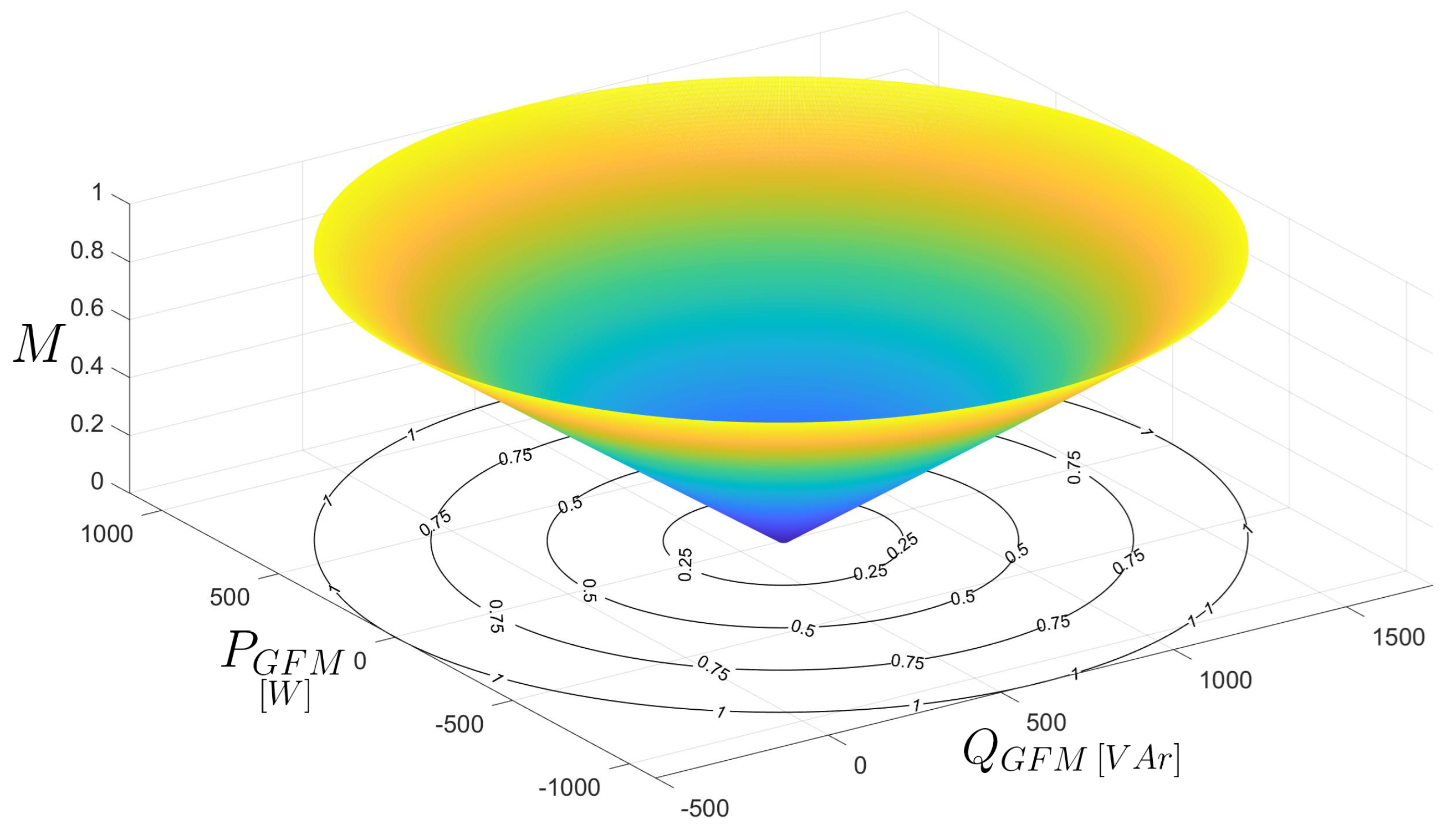
4. Operating Region of a Grid-Connected CSI

4.1. Equations to Find the Operating Region

If the filter capacitance values are chosen with a design ratio of $C_1=2C_2$ for the sake of analytical convenience, assuming that $\omega$ is in a steady state (remains without variation) and taking into account expressions (14) to (16), we can express the currents $i_o^d$ and $i_o^q$ as follows:

$${\mathbf{i}}_{\mathbf{o}}^{\mathbf{dq}}=\left[\begin{array}{c}{i}_o^d\\ i_o^q\end{array}\right]=\left[\begin{array}{c}{v}_{c2}^q{\sigma }_1+i_L^d{\sigma }_2\\ -v_{c2}^d{\sigma }_1+i_L^q{\sigma }_2\end{array}\right],$$

(19)

where

$$\begin{array}{c}{\sigma }_1=\left(2C_2{L}_f{\omega }^2-3\right)\omega C_2\hfill \\ {\sigma }_2=\left(1-2C_2{L}_f{\omega }^2\right)\hfill \end{array}\}.$$

(20)

Assuming the magnitude and phase of the modulators (M and $\varphi$) as inputs provided by a control system, the DC current value ($I_{dc}$), and the grid voltages ($v_g^d$ and $v_g^q$, which are the d and q voltages at the point where the converter connects to the network), are known or measurable, one can derive a system of four nonlinear equations with four unknown variables. This derivation involves considering Equations (14) and (19), and setting the expressions outlined in (18) to zero. The resultant system can be concisely represented as follows:

$$\begin{array}{c}{f}_1({\mathbf{v}}_{\mathbf{c}\mathbf{2}}^{\mathbf{dq}},{\mathbf{i}}_{\mathbf{L}}^{\mathbf{dq}})=v_{c2}^q{\sigma }_1+i_L^d{\sigma }_2-M_G{I}_{dc}sin\left({\varphi }_r\right)=0\hfill \\ f_2({\mathbf{v}}_{\mathbf{c}\mathbf{2}}^{\mathbf{dq}},{\mathbf{i}}_{\mathbf{L}}^{\mathbf{dq}})=-v_{c2}^d{\sigma }_1+i_L^q{\sigma }_2+M_G{I}_{dc}cos\left({\varphi }_r\right)=0\hfill \\ f_3({\mathbf{v}}_{\mathbf{c}\mathbf{2}}^{\mathbf{dq}},{\mathbf{i}}_{\mathbf{L}}^{\mathbf{dq}})=-v_g^d+L_{lin}\omega i_L^q+v_{c2}^d-r_{lin}{i}_L^d=0\hfill \\ f_4({\mathbf{v}}_{\mathbf{c}\mathbf{2}}^{\mathbf{dq}},{\mathbf{i}}_{\mathbf{L}}^{\mathbf{dq}})=-v_g^q-L_{lin}\omega i_L^d+v_{c2}^q-r_{lin}{i}_L^q=0\hfill \end{array}\}.$$

(21)

Subsequently, by considering a control input where the modulator’s magnitude (M) and phase (${\varphi }_r$) are held constant in a steady state and assuming a nominal grid voltage, solving the system described above allows for the identification of an operating point.

It is important to note that, with the determined voltage and current values, one can calculate the active power ($P_{GFM}$) and reactive power ($Q_{GFM}$) that the inverter is capable of delivering or absorbing through the CLC filter as follows:

$$\left[\begin{array}{c}{P}_{GFM}\\ Q_{GFM}\end{array}\right]=\frac{3}{2}\left[\begin{array}{c}{v}_{c2}^d{i}_L^d+v_{c2}^q{i}_L^q\\ v_{c2}^q{i}_L^d-v_{c2}^d{i}_L^q\end{array}\right].$$

(22)

The magnitude of the voltage, at the filter output itself, can also be determined as follows:

$${\widehat{V}}_{GFM}=\sqrt{{\left(v_{c2}^d\right)}^2+{\left(v_{c2}^q\right)}^2}$$

(23)

Finally, the magnitude of the inverter output current will also be relevant from a practical point of view, as this will allow the correct selection of the semiconductors needed in the converter. This magnitude can be derived from Equation (14) and can be written as follows:

$${\widehat{I}}_O=M_G{I}_{dc}.$$

(24)

By evaluating all possible inputs from the system controller—varying the modulator’s magnitude M from 0 to 1, varying the phase $\varphi$ between $-\pi$ and $\pi$, and considering a nominal grid voltage—a comprehensive set of solutions can be obtained by solving the system outlined in (21) for each input configuration. These solutions collectively define what we can refer to as the full operating region, a comprehensive map of potential operating points.

Solutions can be obtained by knowing the fixed parameters and variables of a specific CSI for which the analysis is desired. For instance, in this study, an operating region can be determined for a small prototype inverter being implemented in the laboratory. The prototype has the data from

Table 2. Parameters and fixed variables for the CSI in this document.

Parameter or Variable	Description	Values
$I_{dc}$	DC Source Current	$7\mathrm{A}$
$C_1$	Filter capacitor 1	$60\mathsf{\mu }$F
$C_2$	Filter capacitor 2	$30\mathsf{\mu }$F
$L_f$	Filter inductance	5 m H
$G_{ac}$	Modulation gain	$0.866$
${\widehat{V}}_{nom}$	Output magnitude voltage	120 V

.

4.2. Operating Region for a Specific Grid-Forming CSI

Considering the system of equations provided by the expressions in (21), and taking into account specific parameters and characteristics of the grid-connected CSI converter, including the sizes of capacitances and inductances in the CLC filter, the current $I_{dc}$, modulation type, gain $G_{ac}$, and the magnitude of the nominal operating voltage ${\widehat{V}}_{nom}$, in Table 2, the system can be solved numerically. For each input involving a value M and its phase $\varphi$ applied to the equations in (21), the solution can be achieved by employing the Levenberg–Marquardt method in Matlab, thus determining the voltages and currents in dq axes (${\mathbf{v}}_{\mathbf{c}\mathbf{2}}^{\mathbf{dq}},{\mathbf{i}}_{\mathbf{L}}^{\mathbf{dq}}$).

After the procedures described above are completed, it is possible to compute each solution’s active and reactive powers according to Equation (22), using the obtained values for voltages and currents. By systematically evaluating all possible inputs for the modulator M and its phase $\varphi$ and calculating the corresponding pairs of power values $P_{GFM}$ and $Q_{GFM}$, these powers can be graphically represented as functions of the modulator’s magnitude. The results are depicted in Figure 5.

By focusing on specific iso-value contours that represent the modulation index (M) and projecting them onto the $xy$-plane, where the active and reactive powers of the inverter are depicted, as demonstrated in Figure 5, well-defined limits become evident for the achievable power levels associated with the converter listed in Table 2. It is worth noting that when $M=1$, it becomes apparent that the lowest attainable reactive power for this particular converter remains below $-500\mathrm{VAr}$. A clearer illustration related to the above is shown in Figure 6.

As observed in Figure 5 and Figure 6, there is a substantial operating region for power, characterized by a circular shape within the reactive and active power plane. This pattern suggests a symmetric potential for power output from the converter, with consistent limits radiating in every direction from the center. However, from a practical perspective, control strategies for grid-forming converters, aimed at controlling the output voltage with reference to the active and reactive powers, typically have an operating range for modulation angles that is limited to only two quadrants. This occurs because synchronization is achieved through the active power, and with these control schemes, only one power-frequency pair is feasible for synchronization. In the region identified, there are two potential operating points with the same active power value, dependent on the ${\varphi }_r$ angle of the control system. Consequently, the control can only achieve synchronism with the powers produced in the first and second quadrants of the modulators. A similar situation is observed with synchronous machines, which can operate with their load angles only in two quadrants; outside these quadrants, synchronism is lost [44,45].

Analysis of the data from the operating region reveals distinct active power values $P_{\mathrm{GFM}}$ as functions of the modulator angle ${\varphi }_r$ across various modulation indices M, as illustrated in Figure 7. For each modulation index M, there are typically two possible active power values, except at the extremes; the maximum active power is attained when ${\varphi }_r=0$, and the minimum is observed at ${\varphi }_r=\pi$.

In control strategies analogous to those used in synchronous machines—such as the droop control, power synchronization control (PSC), or virtual synchronous machine control (VSM) strategies—the modulator phase angle plays a critical role similar to the power angle in synchronous machines [46]. It is understood that decreasing the modulator phase angle beyond zero radians risks losing synchrony, just as increasing it beyond $\pi$ radians would. Consequently, the operational region for phase angles is inherently bounded between 0 and $\pi$ radians to maintain synchronism.

Taking into account the above-described range for modulation angle, the entire region can be delineated and segmented into two zones: the sync-guaranteed region, where synchronization is assured, and the out-of-sync region, where synchronization cannot be guaranteed. The resulting graph is shown in Figure 8.

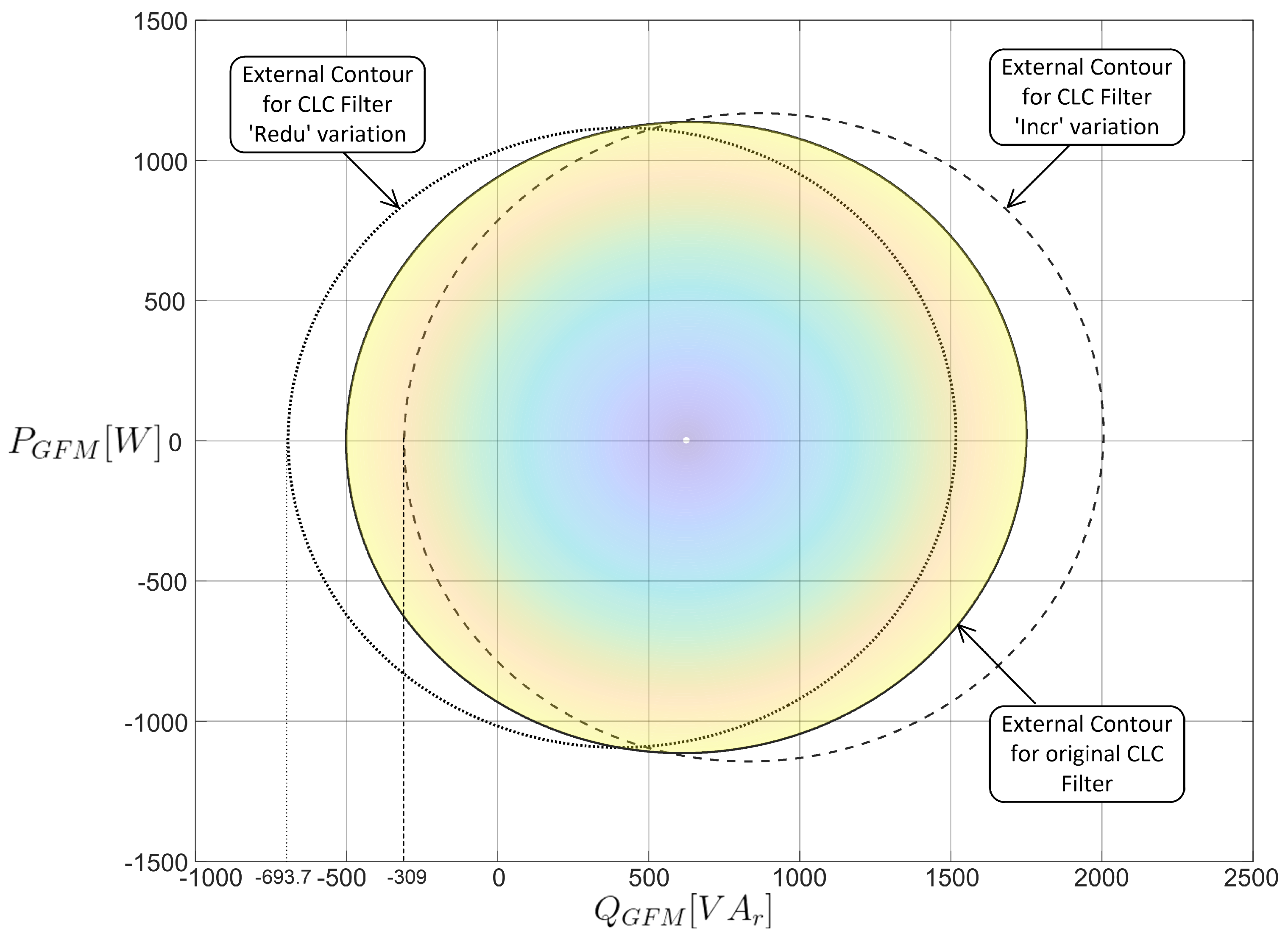
4.3. Effects of CLC Filter Design Variations on the Operating Region

It is important to note that the external contour and the complete operating region can shift, expand, or contract in the power plane depending on the design parameters of the CLC filter, the system’s operating frequency, or the magnitude of the DC current. For example, if one compares the external contour of the operating region obtained with the CLC filter parameters from Table 2 with the contours of two regions obtained by varying the CLC filter parameters, a variation referred to in this document as ‘Redu’, which corresponds to a reduction in the size of the CLC filter, with filter values given as $C_1=40\mathsf{\mu }$F, $C_2=20\mathsf{\mu }$F, and $L_f=3$ mH, and another variation referred to in this document as ‘Incr’, with an increase in the size of the filter, with CLC filter values given as $C_1=80\mathsf{\mu }$F, $C_2=40\mathsf{\mu }$F, and $L_f=7$ mH. By obtaining the external contours of the operating regions for $M=1$ of these two variations and superimposing them with the region obtained for Table 2, it is possible to see in Figure 9 that in the case of the ‘Redu’ variation (filter with reduced values), the converter’s region will shift to the left, allowing it to absorb a greater magnitude of reactive power if desired but reducing the maximum and minimum possible values of active power. On the other hand, if the operating region is obtained with the filter parameters of the ‘Incr’ variation (filter with increased values), the external contour and the operating region will shift to the right, reducing the maximum reactive power absorption capacity but increasing the maximum and minimum active powers that the converter could supply or absorb.

In summary, obtaining the operating region for the CSI with a CLC filter allows for the evaluation of different filter designs by analyzing the external contours, as well as determining the maximum and minimum power levels, which, in part, will depend on the specific parameter designs.

5. Corroborating Results and Simulations of the Model and Operating Region

Simulation serves as an invaluable method for validating the operation of the CSI converter, utilizing the control strategy depicted in Figure 3. This validation ensures that the operating region identified aligns seamlessly with the proposed system configuration. In this study, five potential reference points have been selected for operational validation, as detailed in

Table 3. Power references given for the operating points to be analyzed in simulations.

Operating Point Name	Active Power (${\mathit{P}}_{\mathit{GFM}}$)	Reactive Power (${\mathit{Q}}_{\mathit{GFM}}$)
Test Point R	$-300\mathrm{W}$	$-460\mathrm{VAr}$
Test Point S	$585\mathrm{W}$	$595\mathrm{VAr}$
Test Point T	$229\mathrm{W}$	$464\mathrm{VAr}$
Test Point RE	$281.9\mathrm{W}$	$626.9\mathrm{VAr}$
Test Point OS	$229\mathrm{W}$	$790.8\mathrm{VAr}$

. In the initial section of this chapter, three distinct operating points are carefully chosen and subjected to comprehensive testing within this region. These tests include (i) test point R, located at the left boundary of the region, achieving a modulation value close to $M=1$; (ii) test point S, exploring an operating point near the right edge, with a modulation value of $M=0.5$; and (iii) test point T, assessing an operating point with a lower modulation value of $M=0.25$, slightly further from the right edge than the second case. Following these steady-state tests, three dynamic response tests will be conducted, involving transitions between these points. Finally, the results will be discussed in a concise yet insightful manner.

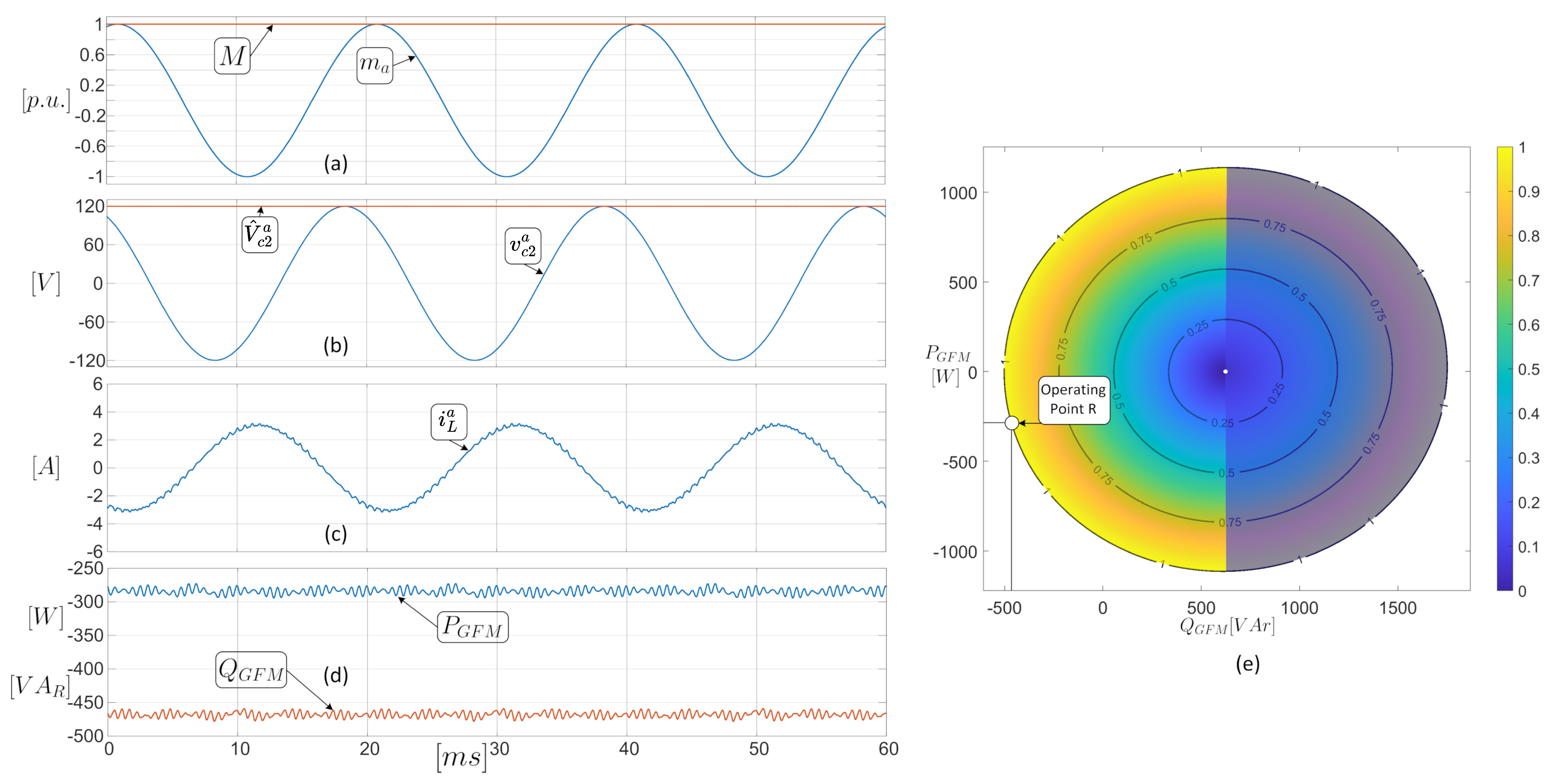
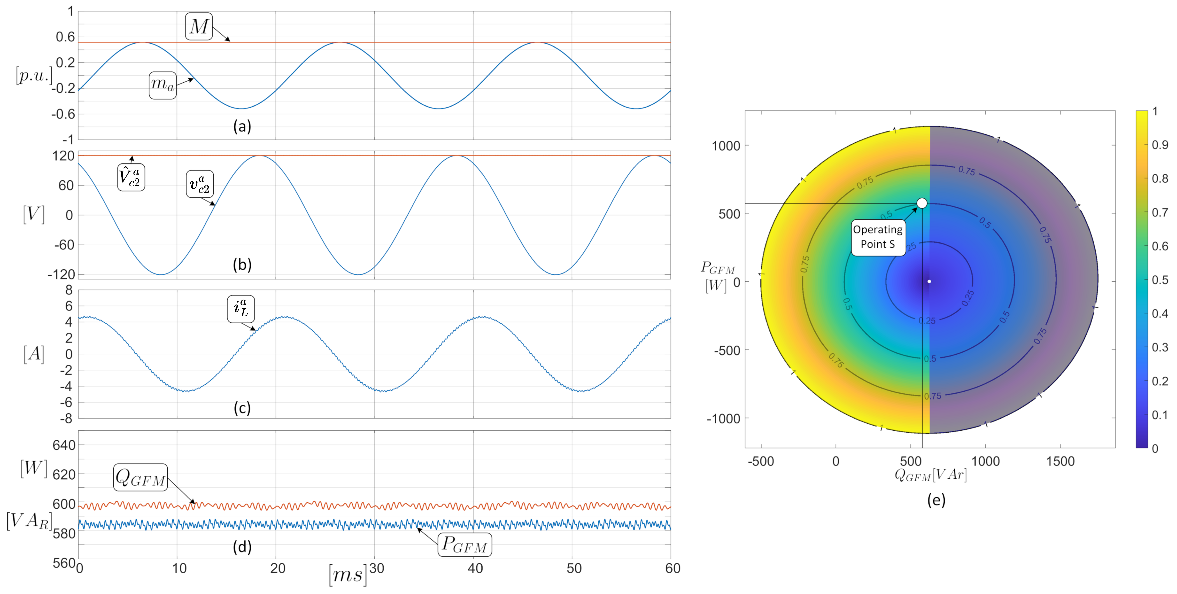
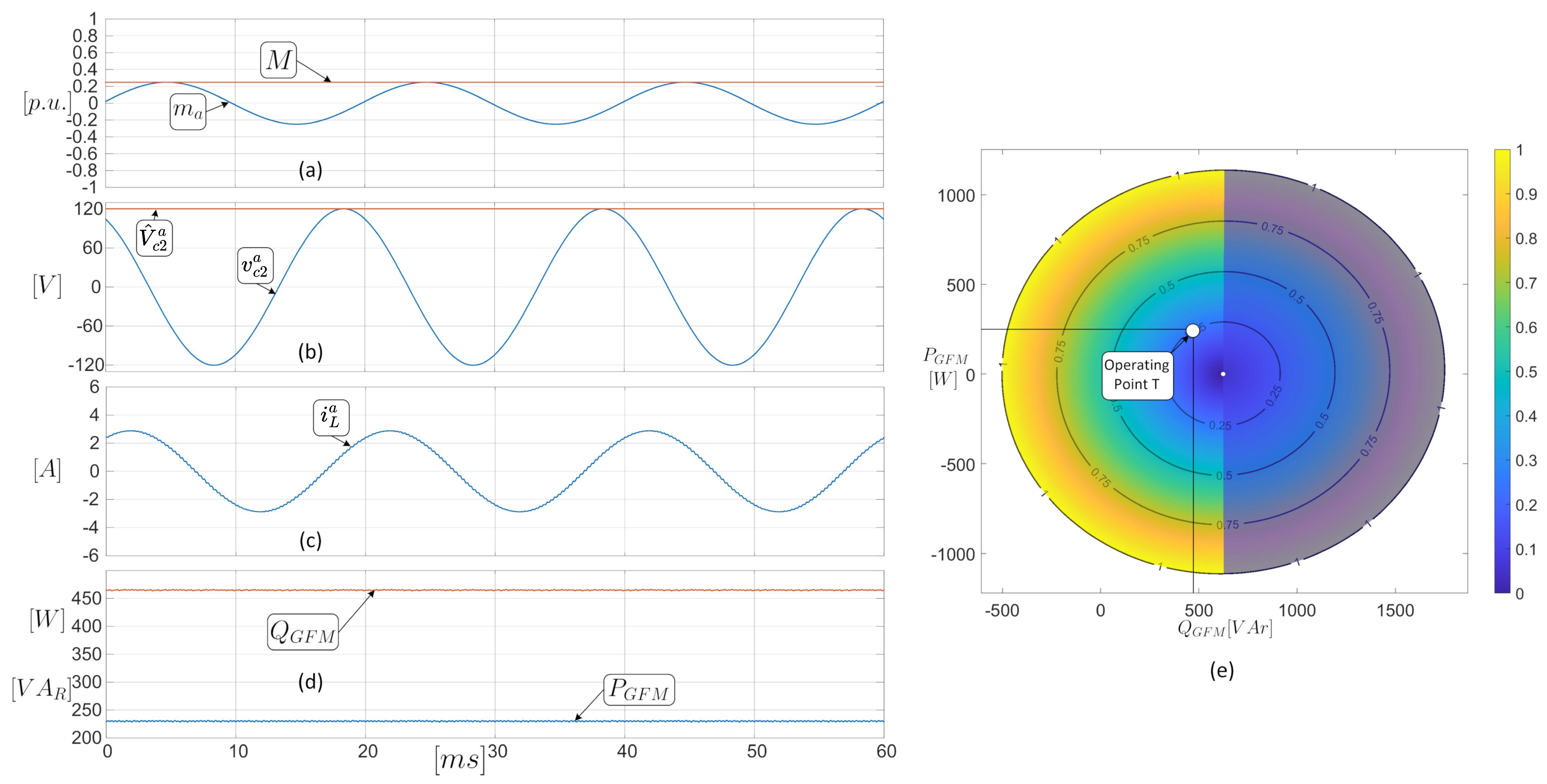
5.1. Steady State Tests

In the initial simulated scenario, Test 1 at test point R, the control system is configured to have the converter absorb both active and reactive power—approximately $-300\mathrm{W}$ and $-460\mathrm{VAr}$, respectively. If, through the references, there were a request for slightly less active or reactive power, the control would lead to over-modulation (a value of M greater than 1). Figure 10’s left panel displays waveforms that include the modulation signal $m_a$ and its magnitude M, as well as the voltage in phase a and its magnitude (see Figure 10b), the load current in line a (Figure 10c), and the recorded values of active and reactive powers (Figure 10d). On the right side of Figure 10, the operating region plots illustrate potential power data along the x and y axes relative to the modulation index M. The operating point where $M=1$ is marked, aligning the active and reactive power values from the simulation in Figure 10d with the axes.

In the second simulated scenario, Test 2 at test point S, the control scheme is adjusted to set the converter to deliver specific positive power levels: $585\mathrm{W}$ of active power and $595\mathrm{VAr}$ of reactive power. On the left side of Figure 11, fundamental waveforms are once again visible: the modulator a, its modulation index M, the voltage waveform in phase a and its magnitude, and the output current in line a. Additionally, the measured active and reactive powers are displayed in Figure 11d. Analysis of the operating region indicates that the operating point is within the synchronization-guaranteed region but quite close to the limit where the out-of-sync region begins, with the modulation index magnitude set at $M=0.5$. This is corroborated by both Figure 11a from the simulation and Figure 11e within the operating region. The measured active and reactive power values at the converter’s output precisely match the corresponding point within the system’s operating area.

In the third simulated experiment, Test 3 at test point T, the control scheme adjusts the power references to achieve a modulation index (M) of $0.25$, thus positioning the operating point further from the boundary where the out-of-sync region begins, compared to the previous case. The active and reactive power values are set at $229\mathrm{W}$ and $464\mathrm{VAr}$, respectively. Figure 12 showcases the modulators, the phase ‘a’ voltage, the load line ‘a’ current, and both active and reactive power readings. An examination of Figure 12a and the power values in Figure 12d which are stably maintained by the droop control proposed in Figure 3 clearly indicates that the modulation and power values are in line with the predictions from the operating region, as illustrated in Figure 12e.

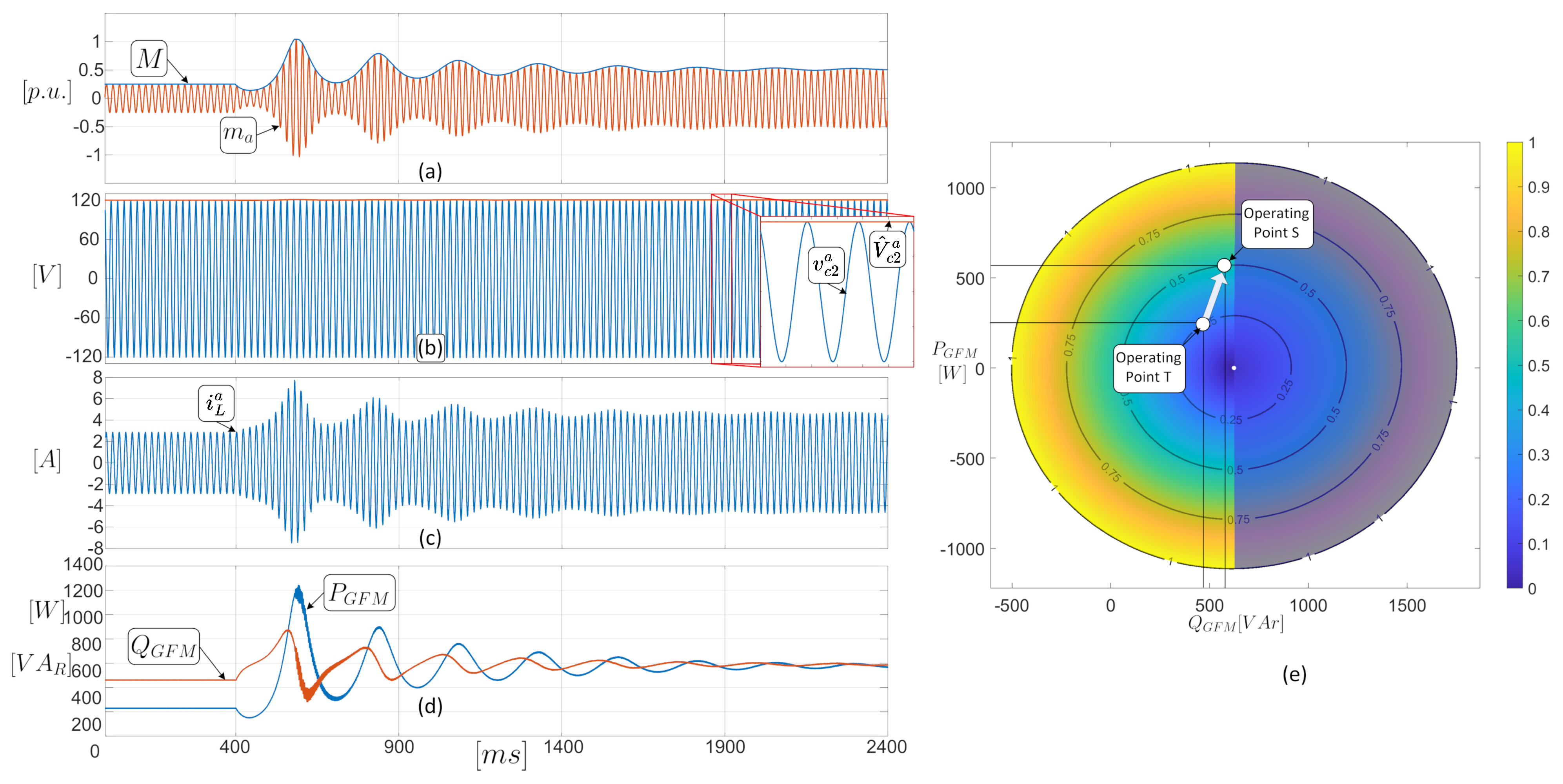
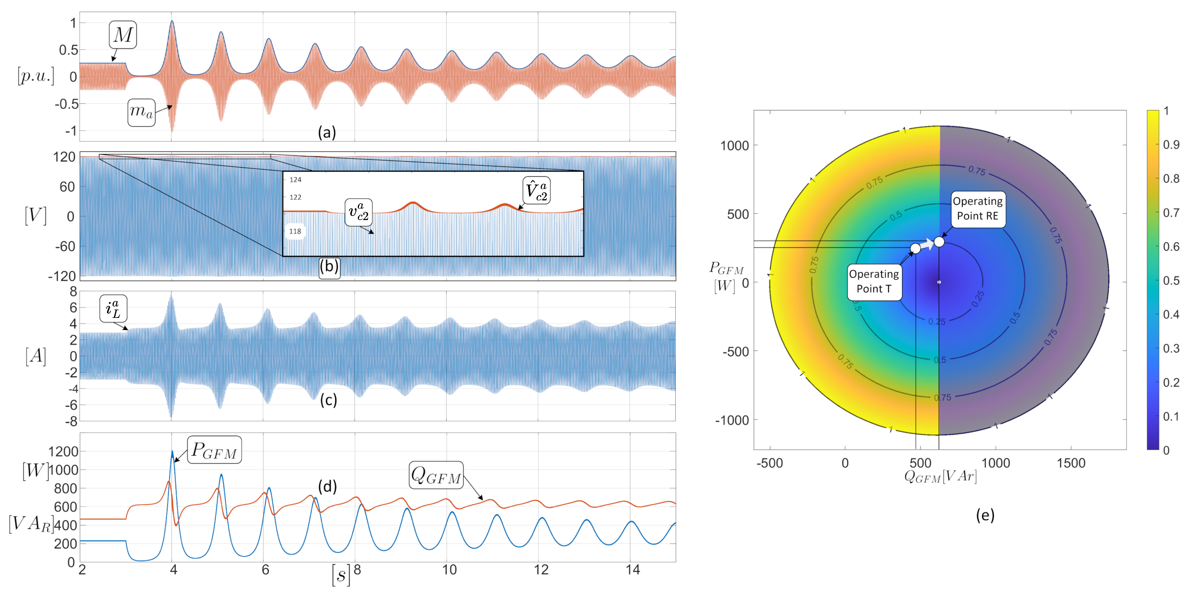
5.2. Test in Transient State

To assess dynamic changes within and outside the operating region, four simulation tests are conducted using the control strategy depicted in Figure 3. Dynamic Test 1 evaluates the system’s response to a step change from test point T to test point R. Dynamic Test 2 assesses the response to a step change from T to S. It should be noted that these three points, R, S, and T, were previously analyzed statically in the initial tests. Dynamic Test 3 examines the response to a step change from T to an operating point at the right edge, designated as RE. Finally, Dynamic Test 4 investigates the system’s response to a step change from T to an operating point OS in the out-of-sync region.

In Dynamic Test 1, as illustrated in Figure 13, the modulator M transitions from a value of 0.25 to 1 per unit (p.u.) at $t=50$ ms, moving from test point T to test point R. The inverter output voltage remains close to the nominal value, while transients are observed in both current and power. Initially, the active and reactive powers are $P_{{\mathrm{GFM}}_T}=229\mathrm{W}$ and $Q_{{\mathrm{GFM}}_T}=464\mathrm{VAr}$, respectively. These values shift to $P_{{\mathrm{GFM}}_R}=-300\mathrm{W}$ and $Q_{{\mathrm{GFM}}_R}=-460\mathrm{VAr}$, indicating that both power outputs in the converter transition from positive to negative values.

Dynamic Test 2 introduces a subtle shift from operating point T with $M=0.25$ p.u. to operating point S with $M=0.5$ p.u. This latter point is near the boundary where synchronism might be compromised. As seen in Figure 14, upon initiating the change in the control system at t = 400 ms, the modulator magnitude exhibits an underdamped response. Similarly, the active and reactive powers in the converter undergo an underdamped transition from point T to point S but stabilize by $t=1900$ ms. Notably, during this transient response, the system’s damping characteristics diminish as the operating point moves from a region far from the out-of-sync boundary toward it.

In Dynamic Test 3, the observations noted at the end of the previous paragraph are confirmed. This test involves transitioning from operating point T, with $M=0.25$ p.u., to an operating point designated as RE, also at $M=0.25$ p.u., located very close to the onset of the out-of-sync region. As illustrated in Figure 15, the waveforms of the modulator, currents, and powers display a highly underdamped response, far more pronounced than the responses observed in Figure 14.

Observations from the last responses (from Figure 14 and Figure 15) suggest that transitioning from an operating point within the sync-guaranteed region into the out-of-sync region may lead to control divergence. This is because proposing power references that are closer to the limit between the synchronized zones and the out-of-sync zone results in increasingly oscillatory responses or reduced damping. In Dynamic Test 4, to further demonstrate the effect of not imposing limits on the control and to illustrate the outcomes when the system operates without constraints, the upper and lower limits of the PI controller, as well as any possible limit on the reactive power reference, have been removed. The behavior of the modulator M is clearly evident when attempting to transition from operating point T to operating point OS, as depicted in Figure 16. This transition results in indefinite divergence immediately after the change at time $t=400$ ms. Furthermore, the responses in the currents and powers, illustrated in Figure 16, degrade, losing the expected quality following the reference change. Consequently, it is clear that operating at test point OS is unable to sustain satisfactory performance.

6. Discussion and Comments

6.1. Overview of Results

A critical observation when analyzing the operating region of a grid-connected CSI under a droop control strategy, particularly during simulations across various points within the area, is that not all sets of points deduced through mathematical modeling are feasible for inverter operation. This study has enabled the determination that by exploring possible inputs—namely, the different modulation indices and angles delivered by the system control—a specific operating point corresponding to particular active and reactive power values can be established for each input. By plotting all these operating points on a plane and projecting the modulation indices onto a third axis, a conical surface is obtained, as seen in Figure 5. Projecting the modulation index values onto the power plane reveals an operational region in a circular shape, as illustrated in Figure 6. However, given that droop control directly correlates the inverter’s power with the system’s frequency, synchronization is achieved through power control by only one pair of power-frequency when the inverter is synchronized with the grid. This results in the operating region being divided into two halves: one with synchronization and the other without.

The steady-state simulations confirm that the model precisely matches the tested system, achieving the active and reactive powers exactly as predicted for the given modulation indices in the operational region. Three operating points were tested: two delivering active and reactive power and one absorbing both. During transitions, or more precisely, in transient state testing, it becomes evident that moving away from the boundary dividing the guaranteed synchronism zone from the non-synchronization zone results in more damped responses as opposed to moving towards it. Transitions from points further away to those closer to the boundary lead to completely underdamped responses. Notably, within the limit zone, where synchronization is not ensured, the operation of the converter becomes compromised.

6.2. Enhancements from Operating Region Insights

By identifying and analyzing the operating region of a CSI converter through modeling and simulation, as demonstrated in this work, there is a chance to select components more effectively. This is because the approach allows for analyzing how the region changes with different component values, enabling the determination of maximum currents through the semiconductors and the maximum and minimum power levels manageable by this inverter. In this regard, recent articles discuss the design and parameter optimization of CSIs [47,48]. This work can be considered complementary to those articles, as it proposes a method to obtain the operating region of a CSI in the active and reactive power plane, facilitating the evaluation of a particular design or the comparison with other designs. Furthermore, understanding these limitations facilitates the integration of appropriate protections directly into the control system. For example, knowing that there is an almost vertical line of reactive power, which divides the zone where synchronization is guaranteed from the zone where it is not, enables the use of the line’s minimum value and, considering a safety margin, limits the reactive power in the control scheme reference. Thus, if secondary control demands a reactive power greater than what the converter can handle, a thorough analysis ensures that the reactive power is capped, preventing system desynchronization due to an incorrect reference change. Additionally, the output of the PI control in the reactive power control loop can be precisely limited to prevent modulation index M values from exceeding set maximums.

7. Conclusions

A grid-connected current source inverter (CSI) equipped with a CLC filter can function as a grid-forming inverter using a droop control strategy. This control scheme only requires voltage and frequency loops, thus eliminating the need for an inner current loop within its control architecture. This operational capability, arising from the current source converter topology’s inherent current management, significantly boosts hardware protection, particularly under conditions such as short circuits or when current demands exceed the inverter’s operational threshold. By employing a precise system model, an operating region is clearly defined, enabling the identification of specific maximum and minimum operational parameters crucial for the practical system design. This process involves calculating potential active and reactive power outputs or the inverter’s maximum current limits based on the modulation indices issued by the system controller.

Simulation results confirm the model’s accuracy and indicate that not all areas within the obtained region can maintain synchronization with the connected electrical grid. A thorough understanding of this operational area allows for setting prudent limits on control scheme references, thereby preventing operations in zones where synchronization is lost or where the modulation index (M) exceeds 1. This study presents a method for methodically acquiring and analyzing the operating region of a CSI with a CLC filter connected to a stiff grid. By analyzing the operating region with the same converter, it is observed that reducing the nominal size of the CLC filter capacitances by 33% allows the system to absorb up to 39% more reactive power. Conversely, increasing the capacitance size by 33% reduces the system’s capacity to absorb reactive power to 62% of its original capacity. This approach opens the door for further detailed analyses or assessments of the impacts of various CLC filter parameters on the system’s active and reactive power capabilities. Future work will involve analyzing the converter’s operating region when it is fully isolated or operating in an isolated microgrid, as this aspect was not considered in the current study. This analysis will complement the results obtained and allow for a comparison of the operating regions of the CSI and VSI converters, providing insights into the performance of both topologies in the power plane.

References

1. Zhang, H.; Xiang, W.; Lin, W.; Wen, J. Grid Forming Converters in Renewable Energy Sources Dominated Power Grid: Control Strategy, Stability, Application, and Challenges. J. Mod. Power Syst. Clean Energy 2021, 9, 1239–1256. [Google Scholar] [CrossRef]
2. Peña Asensio, A.; Arnaltes Gómez, S.; Rodriguez-Amenedo, J.L. Black-start capability of PV power plants through a grid-forming control based on reactive power synchronization. Int. J. Electr. Power Energy Syst. 2023, 146, 108730. [Google Scholar] [CrossRef]
3. Sawant, J.; Seo, G.S.; Ding, F. Resilient Inverter-Driven Black Start with Collective Parallel Grid-Forming Operation. In Proceedings of the 2023 IEEE Power & Energy Society Innovative Smart Grid Technologies Conference (ISGT), Washington, DC, USA, 16–19 January 2023; pp. 1–5. [Google Scholar] [CrossRef]
4. Rocabert, J.; Luna, A.; Blaabjerg, F.; Rodríguez, P. Control of Power Converters in AC Microgrids. IEEE Trans. Power Electron. 2012, 27, 4734–4749. [Google Scholar] [CrossRef]
5. Henninger, S.; Jaeger, J. Advanced classification of converter control concepts for integration in electrical power systems. Int. J. Electr. Power Energy Syst. 2020, 123, 106210. [Google Scholar] [CrossRef]
6. Lai, N.B.; Tarrasó, A.; Baltas, G.N.; Marin Arevalo, L.V.; Rodriguez, P. External Inertia Emulation Controller for Grid-Following Power Converter. IEEE Trans. Ind. Appl. 2021, 57, 6568–6576. [Google Scholar] [CrossRef]
7. Strunz, K.; Almunem, K.; Wulkow, C.; Kuschke, M.; Valescudero, M.; Guillaud, X. Enabling 100% Renewable Power Systems Through Power Electronic Grid-Forming Converter and Control: System Integration for Security, Stability, and Application to Europe. Proc. IEEE 2023, 111, 891–915. [Google Scholar] [CrossRef]
8. Peng, F.Z.; Liu, C.C.; Li, Y.; Jain, A.K.; Vinnikov, D. Envisioning the Future Renewable and Resilient Energy Grids—A Power Grid Revolution Enabled by Renewables, Energy Storage, and Energy Electronics. IEEE J. Emerg. Sel. Top. Ind. Electron. 2024, 5, 8–26. [Google Scholar] [CrossRef]
9. Hossain, E.; Faruque, H.M.R.; Sunny, M.S.H.; Mohammad, N.; Nawar, N. A Comprehensive Review on Energy Storage Systems: Types, Comparison, Current Scenario, Applications, Barriers, and Potential Solutions, Policies, and Future Prospects. Energies 2020, 13, 3651. [Google Scholar] [CrossRef]
10. Ellis, B.E.; Pearre, N.; Swan, L. Impact of residential photovoltaic systems on net load intermittency. Renew. Energy Focus 2023, 46, 377–384. [Google Scholar] [CrossRef]
11. Unruh, P.; Nuschke, M.; Strauß, P.; Welck, F. Overview on grid-forming inverter control methods. Energies 2020, 13, 2589. [Google Scholar] [CrossRef]
12. Safamehr, H.; Izadi, I.; Ghaisari, J. Robust VI Droop Control of Grid-Forming Inverters in the Presence of Feeder Impedance Variations and Nonlinear Loads. IEEE Trans. Ind. Electron. 2024, 71, 504–512. [Google Scholar] [CrossRef]
13. Liu, T.; Wang, X. Unified Voltage Control for Grid-Forming Inverters. IEEE Trans. Ind. Electron. 2024, 71, 2578–2589. [Google Scholar] [CrossRef]
14. Rosso, R.; Wang, X.; Liserre, M.; Lu, X.; Engelken, S. Grid-Forming Converters: Control Approaches, Grid-Synchronization, and Future Trends—A Review. IEEE Open J. Ind. Appl. 2021, 2, 93–109. [Google Scholar] [CrossRef]
15. Pattabiraman, D. Current source inverter with grid forming control. Electr. Power Syst. Res. 2024, 226, 109910. [Google Scholar] [CrossRef]
16. Abdel-Moneim, M.G.; Hamad, M.S.; Abdel-Khalik, A.S.; Hamdy, R.R.; Hamdan, E.; Ahmed, S. Analysis and control of split-source current-type inverter for grid-connected applications. Alex. Eng. J. 2024, 96, 268–278. [Google Scholar] [CrossRef]
17. Xu, C.; Liu, P.; Miao, Y. Overlap Time Compensation and Characteristic Analysis for Current Source Photovoltaic Grid-Connected Inverter. Energies 2024, 17, 1768. [Google Scholar] [CrossRef]
18. Gao, H. High-frequency common-mode voltage mitigation for current-source inverter in transformerless photovoltaic system using active zero-state space vector modulation. IET Electr. Power Appl. 2023, 17, 245–255. [Google Scholar] [CrossRef]
19. Geng, Y.; Zhou, T.; Cao, F.; Xin, Y.; Wang, H. A model predictive control of three-phase grid-connected current-source inverter based on optimization theory. IET Power Electron. 2023, 16, 2650–2665. [Google Scholar] [CrossRef]
20. Ray, I. Review of Impedance-Based Analysis Methods Applied to Grid-Forming Inverters in Inverter-Dominated Grids. Energies 2021, 14, 2686. [Google Scholar] [CrossRef]
21. Lasseter, R.H.; Chen, Z.; Pattabiraman, D. Grid-Forming Inverters: A Critical Asset for the Power Grid. IEEE J. Emerg. Sel. Top. Power Electron. 2020, 8, 925–935. [Google Scholar] [CrossRef]
22. Young, H.A.; Marin, V.A.; Pesce, C.; Rodriguez, J. Simple Finite-Control-Set Model Predictive Control of Grid-Forming Inverters With LCL Filters. IEEE Access 2020, 8, 81246–81256. [Google Scholar] [CrossRef]
23. Geng, Y.; Yang, K.; Lai, Z.; Zheng, P.; Liu, H.; Deng, R. A Novel Low Voltage Ride Through Control Method for Current Source Grid-Connected Photovoltaic Inverters. IEEE Access 2019, 7, 51735–51748. [Google Scholar] [CrossRef]
24. Alemi, P.; Wang, J.; Zhang, J.; Amini, S. Performance analysis of high-power three-phase current source inverters in photovoltaic applications. IET Circuits Devices Syst. 2021, 15, 79–87. [Google Scholar] [CrossRef]
25. Fidone, G.L.; Migliazza, G.; Carfagna, E.; Benatti, D.; Immovilli, F.; Buticchi, G.; Lorenzani, E. Common Architectures and Devices for Current Source Inverter in Motor-Drive Applications: A Comprehensive Review. Energies 2023, 16, 5645. [Google Scholar] [CrossRef]
26. Killeen, P.; Ghule, A.N.; Ludois, D.C. A Medium-Voltage Current Source Inverter for Synchronous Electrostatic Drives. IEEE J. Emerg. Sel. Top. Power Electron. 2022, 10, 1597–1608. [Google Scholar] [CrossRef]
27. Migliazza, G.; Buticchi, G.; Carfagna, E.; Lorenzani, E.; Madonna, V.; Giangrande, P.; Galea, M. DC Current Control for a Single-Stage Current Source Inverter in Motor Drive Application. IEEE Trans. Power Electron. 2021, 36, 3367–3376. [Google Scholar] [CrossRef]
28. Azmi, S.A.; Ahmed, K.H.; Finney, S.J.; Williams, B.W. Comparative analysis between voltage and current source inverters in grid-connected application. In Proceedings of the IET Conference on Renewable Power Generation (RPG 2011), Edinburgh, UK, 6–8 September 2011; pp. 1–6. [Google Scholar] [CrossRef]
29. Sahan, B.; Araújo, S.V.; Nöding, C.; Zacharias, P. Comparative Evaluation of Three-Phase Current Source Inverters for Grid Interfacing of Distributed and Renewable Energy Systems. IEEE Trans. Power Electron. 2011, 26, 2304–2318. [Google Scholar] [CrossRef]
30. Tan, Q.; Mao, L.; Cai, Y.; Zhang, B.; Ruan, Z. Comparative evaluation and analysis of GaN-based VSIs and CSIs. Energy Rep. 2023, 9, 568–576. [Google Scholar] [CrossRef]
31. Dai, H.; Jahns, T.M.; Torres, R.A.; Han, D.; Sarlioglu, B. Comparative Evaluation of Conducted Common-Mode EMI in Voltage-Source and Current-Source Inverters using Wide-Bandgap Switches. In Proceedings of the 2018 IEEE Transportation Electrification Conference and Expo (ITEC), Long Beach, CA, USA, 13–15 June 2018; pp. 788–794. [Google Scholar] [CrossRef]
32. Wang, Z.; Wei, Q. X-Type Five-Level Current Source Inverter. IEEE Trans. Power Electron. 2023, 38, 6283–6292. [Google Scholar] [CrossRef]
33. Wang, Z.; Wei, Q. Γ-Type Five-Level Current Source Inverter. IEEE Trans. Power Electron. 2024, 39, 7206–7216. [Google Scholar] [CrossRef]
34. Kim, J.; Cha, H. Switching Cell Current Source Inverter With Active Power Decoupling Circuit. IEEE Trans. Ind. Electron. 2024, 1–9. [Google Scholar] [CrossRef]
35. Zheng, Z.; Xie, Q.; Huang, C.; Xiao, X.; Li, C. Superconducting Technology Based Fault Ride Through Strategy for PMSG-Based Wind Turbine Generator: A Comprehensive Review. IEEE Trans. Appl. Supercond. 2021, 31, 1–6. [Google Scholar] [CrossRef]
36. Wang, Z.; Jiang, L.; Zou, Z.; Cheng, M. Operation of SMES for the Current Source Inverter Fed Distributed Power System Under Islanding Mode. IEEE Trans. Appl. Supercond. 2013, 23, 5700404. [Google Scholar] [CrossRef]
37. Hassan, M.u.; Emon, A.I.; Luo, F.; Solovyov, V. Design and Validation of a 20-kVA, Fully Cryogenic, Two-Level GaN-Based Current Source Inverter for Full Electric Aircrafts. IEEE Trans. Transp. Electrif. 2022, 8, 4743–4759. [Google Scholar] [CrossRef]
38. Potdukhe, K.C.; Munshi, A.P.; Munshi, A.A. Reliability prediction of new improved current source inverter (CSI) topology for transformer-less grid connected solar system. In Proceedings of the 2015 IEEE Power, Communication and Information Technology Conference (PCITC), Bhubaneswar, India, 15–17 October 2015; pp. 373–378. [Google Scholar] [CrossRef]
39. Marignetti, F.; Di Stefano, R.L.; Rubino, G.; Giacomobono, R. Current Source Inverter (CSI) Power Converters in Photovoltaic Systems: A Comprehensive Review of Performance, Control, and Integration. Energies 2023, 16, 7319. [Google Scholar] [CrossRef]
40. Mustafeez-Ul-Hassan; Emon, A.I.; Yuan, Z.; Peng, H.; Luo, F. Performance Comparison and Modelling of Instantaneous Current Sharing Amongst GaN HEMT Switch Configurations for Current Source Inverters. In Proceedings of the 2022 IEEE Applied Power Electronics Conference and Exposition (APEC), Houston, TX, USA, 20–24 March 2022; pp. 2014–2020. [Google Scholar] [CrossRef]
41. Lin, Y.; Eto, J.H.; Johnson, B.B.; Flicker, J.D.; Lasseter, R.H.; Pico, H.N.V.; Seo, G.S.; Pierre, B.J.; Ellis, A.; Miller, J.; et al. Pathways to the Next-Generation Power System with Inverter-Based Resources: Challenges and recommendations. IEEE Electrif. Mag. 2022, 10, 10–21. [Google Scholar] [CrossRef]
42. Tamrakar, U.; Shrestha, D.; Maharjan, M.; Bhattarai, B.P.; Hansen, T.M.; Tonkoski, R. Virtual Inertia: Current Trends and Future Directions. Appl. Sci. 2017, 7, 654. [Google Scholar] [CrossRef]
43. Melin, P.E.; Espinoza, J.R.; Zargari, N.R.; Sanchez, M.A.; Guzman, J.I. Modeling Issues in Three-Phase Current Source Rectifiers that use Damping Resistors. In Proceedings of the 2006 IEEE International Symposium on Industrial Electronics, Paris, France, 7–10 November 2006; Volume 2, pp. 1247–1252. [Google Scholar] [CrossRef]
44. Basler, M.J.; Schaefer, R.C. Understanding Power-System Stability. IEEE Trans. Ind. Appl. 2008, 44, 463–474. [Google Scholar] [CrossRef]
45. Shuai, Z.; Shen, C.; Liu, X.; Li, Z.; Shen, Z.J. Transient Angle Stability of Virtual Synchronous Generators Using Lyapunov’s Direct Method. IEEE Trans. Smart Grid 2019, 10, 4648–4661. [Google Scholar] [CrossRef]
46. Ippolito, M.G.; Musca, R.; Zizzo, G. Generalized power-angle control for grid-forming converters: A structural analysis. Sustain. Energy Grids Netw. 2022, 31, 100696. [Google Scholar] [CrossRef]
47. Geng, Y.; Song, X.; Zhang, X.; Yang, K.; Liu, H. Stability Analysis and Key Parameters Design for Grid-Connected Current-Source Inverter with Capacitor-Voltage Feedback Active Damping. IEEE Trans. Power Electron. 2021, 36, 7097–7111. [Google Scholar] [CrossRef]
48. Riegler, B.; Muetze, A. Passive Component Optimization for Current-Source-Inverters. IEEE Trans. Ind. Appl. 2023, 59, 6113–6124. [Google Scholar] [CrossRef]
Figure 1. Configuration of inverters operating in various modes within a microgrid.
Mathematics 12 01775 g001
Figure 2. Current source inverter (CSI) and its possible operation as a grid-connected inverter.
Mathematics 12 01775 g002
Figure 3. Droop control scheme for application in a CSI.
Mathematics 12 01775 g003
Figure 4. CSI schematic with variables needed for modeling.
Mathematics 12 01775 g004
Figure 5. Modulator magnitude versus active and reactive powers.
Mathematics 12 01775 g005
Figure 6. Full theoretical operating region for the grid-connected CSI, obtained through contours.
Mathematics 12 01775 g006
Figure 7. Output power versus modulator angle for various modulator magnitudes.
Mathematics 12 01775 g007
Figure 8. Operating regions with guaranteed synchronism and without synchronism for grid-forming strategies for CSI.
Mathematics 12 01775 g008
Figure 9. Shifts in the external contours of the operating region due to changes in CLC filter parameters.
Mathematics 12 01775 g009
Figure 10. Test 1 waveforms and operating points. (a) Modulator and modulator magnitude; (b) output phase voltage of converter and magnitude of this voltage; (c) load current waveform in line ‘a’; (d) active and reactive power of the converter; (e) operating point of the modulator magnitude as seen from its operating region.
Mathematics 12 01775 g010
Figure 11. Test 2 waveforms and operating points. (a) Modulator and modulator magnitude; (b) output phase voltage of converter and magnitude of this voltage; (c) load current waveform in line ‘a’; (d) active and reactive power of the converter; (e) operating point of the modulator magnitude as seen from its operating region.
Mathematics 12 01775 g011
Figure 12. Test 3 waveforms and operating points. (a) Modulator and modulator magnitude; (b) output phase voltage of converter and magnitude of this voltage; (c) load current waveform in line ‘a’; (d) active and reactive power of the converter; (e) operating point of the modulator magnitude as seen from its operating region.
Mathematics 12 01775 g012
Figure 13. Dynamic Test 1 waveforms and operating points. (a) Modulator and modulator magnitude; (b) output phase voltage of converter and magnitude of this voltage; (c) load current waveform in line ‘a’; (d) active and reactive power of the converter; (e) operating point of the modulator magnitude as seen from its operating region.
Mathematics 12 01775 g013
Figure 14. Dynamic Test 2 waveforms and operating points. (a) Modulator and modulator magnitude; (b) output phase voltage of converter and magnitude of this voltage; (c) load current waveform in line ‘a’; (d) active and reactive power of the converter; (e) operating point of the modulator magnitude as seen from its operating region.
Mathematics 12 01775 g014
Figure 15. Dynamic Test 3 waveforms and operating points. (a) Modulator and modulator magnitude; (b) output phase voltage of converter and magnitude of this voltage; (c) load current waveform in line ‘a’; (d) active and reactive power of the converter; (e) operating point of the modulator magnitude as seen from its operating region.
Mathematics 12 01775 g015
Figure 16. Dynamic Test 4 waveforms and operating points. (a) Modulator and modulator magnitude; (b) output phase voltage of converter and magnitude of this voltage; (c) load current waveform in line ‘a’; (d) active and reactive power of the converter; (e) operating point of the modulator magnitude as seen from its operating region.
Mathematics 12 01775 g016