Article

Advanced Copula-Based Models for Type II Censored Data: Applications in Industrial and Medical Settings

1
Department of Mathematics and Statistics, Faculty of Science, Imam Mohammad Ibn Saud Islamic University (IMSIU), Riyadh 11432, Saudi Arabia
2
Department of Statistics, Faculty of Business Administration, Delta University for Science and Technology, Gamasa 11153, Egypt
3
Department of Statistics, Faculty of Science, King Abdulaziz University, Jeddah 21589, Saudi Arabia
4
Department of Statistics, Mathematics and Insurance, Benha University, Benha 13511, Egypt
*
Author to whom correspondence should be addressed.
Mathematics 2024, 12(12), 1774; https://doi.org/10.3390/math12121774
Submission received: 1 April 2024 / Revised: 1 June 2024 / Accepted: 4 June 2024 / Published: 7 June 2024
(This article belongs to the Special Issue Dependence Modeling with Copulas and Their Applications)

Abstract

:
Copula models are increasingly recognized for their ability to capture complex dependencies among random variables. In this study, we introduce three innovative bivariate models utilizing copula functions: the XLindley (XL) distribution with Frank, Gumbel, and Clayton copulas. The results highlight the fundamental characteristics and effectiveness of these newly introduced bivariate models. Statistical inference for the distribution parameters is conducted using a Type II censored sampling design. This employs maximum likelihood and Bayesian estimation techniques. Asymptotic and credible confidence intervals are calculated, and numerical analysis is performed using the Markov Chain Monte Carlo method. The proposed methodology’s applicability is illustrated by analyzing several real-world datasets. The initial dataset examines burr formation occurrences and consists of two observation sets. Additionally, the second and third datasets contain medical information. The second dataset focuses on diabetic nephropathy, while the third dataset explores infection and recurrence time among kidney patients.

1. Introduction

The construction of several bivariate distributions has attracted considerable attention. Bivariate data find applications in a wide range of fields, including engineering, industry, finance, economics, technology, sports, drought, weather, medical sciences, and many more. In recent years, various methods have been explored to generate new bivariate distributions based on different approaches. These methods include the marginal transformation method [1], copula method [2], conditional specification method [3], frailty approach [4], and the Marshall–Olkin methodology [5]. For more in-depth information on these methods and their application in establishing bivariate distributions, one can refer to the works of Ashkar and Aucoin [1], Nelsen [2], Vincent Raja and Gopalakrishnan [4], and Pathak and Vellaisamy [6].
In recent decades, copula theories have witnessed substantial growth in response to the increasing importance placed on modeling and describing diverse relationships among random variables. The emergence of new copula families has been motivated by the need to explore the structure of dependence in various fields, including the insurance industry [7], actuarial science [8,9], finance [10], hydrology [11], and public health and medicine [12], among others. This highlights the recognition of the significance of investigating the patterns of dependence between random variables in these domains.
In the field of statistical literature, copula structures have been widely employed by numerous authors as a method for establishing and modeling bivariate distributions. Flores [13] presented various bivariate Weibull models based on different copula functions, such as the Farlie–Gumbel–Morgenstern (FGM), Clayton, Ali–Mikhail–Haq (AMH), Gumbel–Hougaard, Gumbel–Barnett, and Nelsen Ten copulas. Abd Elaal et al. [14] introduced a bivariate generalized exponential distribution based on the FGM and Plackett copulas. Baharith et al. [15] proposed two bivariate Pareto Type II distributions; one is derived from the Gaussian copula (BPIIG) and the other is based on the mixture and Gaussian copula (BPIImG). El-sherpieny et al. [16] introduced the bivariate generalized Rayleigh distribution, denoted as Clayton-BGR, which is based on the Clayton copula. The study also derived the likelihood function for a progressive Type II censoring scheme with random removal and applied it to the Clayton-BGR distribution. Usman and Aliyu [17] proposed a new bivariate Nadarajah–Haghighi distribution using two copula functions: the Gumbel–Barnett and Clayton copula functions. Qura et al. [18] introduced a bivariate power Lomax distribution, named BFGMPLx, which is based on Farlie–Gumbel–Morgenstern (FGM) copulas. Fayomi et al. [19] presented a novel family of bivariate continuous Lomax generators called the BFGMLG family. This family is constructed by utilizing univariate Lomax generator (LG) families and the Farlie–Gumbel–Morgenstern (FGM) copula. Fayomi et al. [20] introduced two innovative continuous bivariate families, the FGM bivariate Kavya–Manoharan transformation and the Clayton bivariate Kavya–Manoharan transformation families, which are derived from the univariate Kavya–Manoharan transformation family and incorporate FGM and Clayton copulas, respectively.
In numerous life-testing experiments, it is typical for some test units’ lifetimes to remain unobserved. Censored observations arise when a sample is drawn from a complete population, but either the initial or final observations remain unknown. Type I and Type II censoring are the two predominant methods employed. Consider a scenario where n items are simultaneously subjected to a life test, planned to end upon observing the r-th failure (where r is predetermined). Consequently, only the initial r failures are recorded. This kind of data collected from a restricted life test is denoted as a Type II censored sample. In the context of bivariate censoring samples, Balakrishnan and Kim [21] introduced the likelihood function for a bivariate distribution based on Type II censoring. Kim et al. [22] have explored both maximum likelihood and Bayesian estimation methods for determining the unknown parameters in the bivariate generalized exponential distribution under a Type II censoring scheme. Almetwally [23] has explored the estimation of parameters in bivariate models within a specific censoring framework. Bai et al. [24] introduced the Type I progressive interval censoring schemes for the Marshall–Olkin bivariate Weibull (MOBW) distribution and discussed how confidence intervals depend on the percentile bootstrap of the unknown parameters. El-Morshedy et al. [25] have examined both maximum likelihood and Bayesian methods for estimating the parameters of the bivariate Burr X-G family, considering various distributions and utilizing Type II censored data. Lin et al. [26] used the Pareto type I distribution for the joint frailty–copula model, a well-known heavy-tailed distribution. They devised statistical inference techniques encompassing bivariate random censoring, semi-competing risks, and competing risks, alongside maximum likelihood estimation procedures. Haj Ahmed et al. [27] introduced a novel bivariate model based on the FGM copula and the univariate modified extended exponential distribution, named the bivariate modified extended exponential distribution. They estimated the unknown parameters using both maximum likelihood and Bayesian estimation methods within a Type II censored sampling scheme.
The bivariate model, based on a censored sample, holds significant importance in various fields of data science. It facilitates the analysis of the relationship between two variables through copula functions, effectively reducing data collection costs while maintaining overall efficiency comparable to that of using complete samples. In recent times, the analysis of data has become increasingly challenging due to the prevalence of large and diverse datasets. A notable characteristic of these extensive datasets is their frequent redundancy. For further information on data science, refer to the works of Gramaje et al. [28] and Tien [29].
In this study, three novel bivariate distributions were developed using a special mixture of exponential and Lindley distributions, as detailed in Chouia and Zeghdoudi [30]. The specific mixture of exponential and Lindley distributions mentioned is referred to as the XLindley (XL) distribution. This new model features a single parameter, making it easy to use, granting significant flexibility to its density function and suitability for modeling different data patterns. Moreover, it demonstrates an increasing hazard function, making it a valuable tool in various statistical analyses and modeling, as discussed in Chouia and Zeghdoudi [30]. Furthermore, other papers have utilized the XLindley distribution to create new extended distributions, as seen in Ahsan-ul-Haq et al. [31], Etaga et al. [32], Musekwa and Makubate [33], and Gemeay et al. [34]. In the latter, Alotaibi et al. [35] employed an adaptive Type II progressive hybrid censoring plan to tackle estimation challenges related to the XL distribution using both classical and Bayesian methods. Their study illustrated that datasets from chemical engineering could be effectively modeled using the XL distribution instead of traditional distributions such as gamma and Weibull distributions. Additionally, Alotaibi et al. [36] delved into the estimation of constant-stress accelerated life tests (CSALT) for XL distribution based on progressive.
Type II censoring, applying it to model specific engineering domains. Based on previous studies investigating this distribution, it was proven that it is more efficient than many famous competing distributions, such as the Lindley, Xgamma, exponential, Zeghdoudi, log-normal, and Pareto distributions. Therefore, this was a strong motivation to use this distribution to create the best bivariate model.
Considering the above, the main objectives of this paper are as follows:
  • Introducing three innovative models derived from the XLindley distribution and copula functions:
    • The Frank Bivariate XL (FBXL) Distribution;
    • The Gumbel Bivariate XL (GBXL) Distribution;
    • The Clayton Bivariate XL (CBXL) Distribution.
    These novel models offer enhanced flexibility and suitability for application across diverse fields, including the medical and industrial domains.
  • Sub-objectives of this paper include:
    • Examining multiple scenarios based on an XLindley distribution with a single parameter, enabling a more thorough comparison, particularly across various datasets.
    • Estimating the parameters of bivariate XLindley models involves utilizing both maximum likelihood estimation (MLE) and Bayesian estimation methods. This consideration accounts for both complete and censored samples within a Type II framework.
    • Evaluating the estimators of novel bivariate models involves employing numerical techniques such as the Metropolis–Hastings algorithm.
    • Investigating two types of confidence intervals, namely asymptotic intervals and Bayesian credible intervals, for estimating the unknown parameters.
    • Assessing the fit of the bivariate model involves the use of various goodness-of-fit measures.
This study holds significant importance for two critical sectors in any country: the industrial and medical sectors.
In the industrial sector, tasks involving metal sheet manipulation, such as perforating procedures and measurements related to hole diameter and sheet thickness, are essential in metalworking and manufacturing processes. Burr formation, a common occurrence in these processes, is particularly significant for engineers and scientists due to its implications for product quality, manufacturing efficiency, innovation, and cost reduction.
In the healthcare sector, our research focuses on two key areas: diabetic nephropathy and infection recurrence in kidney patients. Understanding the progression of diabetic nephropathy is crucial, as it provides insights into key risk factors and aids in predicting renal complications, thus enabling the optimization of treatment protocols. Similarly, in the analysis of infection recurrence, survival analysis plays a pivotal role in evaluating infections at catheter insertion sites, guiding the optimization of infection management. This knowledge empowers healthcare professionals to refine treatment strategies, make well-informed decisions, and enhance patient outcomes in both diabetic nephropathy and infection recurrence scenarios.
The rest of this paper is organized as follows: Section 2 provides a review of the copula function, along with discussions on the Frank, Gumbel, and Clayton copulas. The FBXL, GBXL, and CBXL distributions are defined in Section 3. In Section 4, maximum likelihood estimation and Bayesian estimation were performed. Section 5 delves into the discussion of confidence intervals. In Section 6, the suitability of the new models is demonstrated through a simulation study. Section 7 discusses the applications of iron material jobs data, diabetic nephropathy data, and kidney patient data. Finally, in Section 8, the conclusion and some remarks regarding the FBXL, GBXL, and CBXL distributions are presented.

2. Copula Function

In this section, the general definition of Archimedean copulas is presented, and the Frank, Gumbel, and Clayton copulas are discussed.
The copula is a convenient approach to describe a bivariate distribution with a dependence structure. The utilization of copulas is motivated by their numerous advantages in analyzing the interdependence between random variables. The copula functions present a flexible framework that allows for capturing diverse dependence patterns, encompassing both linear and non-linear relationships, tail dependencies, and asymmetries. By adopting a “vine copula” approach, copulas effectively separate the modeling of marginal distributions from the modeling of dependence. Additionally, the copulas facilitate the estimation of conditional dependencies, enabling the investigation of the interdependence among the remaining variables. This feature is valuable in risk management, portfolio optimization, and the pricing of complex financial products. Compared to traditional correlation-based approaches, copula models offer a more robust alternative by providing a comprehensive and accurate representation of dependence, particularly in the presence of non-linear relationships or non-normal distributions.
The Sklar theorem, introduced by Sklar [37], plays a crucial role in copula theory. According to this theorem, for two random variables X and Y with marginal cumulative distribution functions (cdfs) denoted as u = F 1 ( x ) and v = F 2 ( y ) , and marginal probability density functions (pdfs) represented as f 1 ( x ) and f 2 ( y ) , respectively, let C θ ( u , v ) represent the copula cdf, and c θ ( u , v ) denote the copula pdf. Then, the joint cdf and joint pdf of (X, Y) based on the copula can be expressed as follows:
F ( x , y ) = C θ F 1 ( x ; Γ 1 ) , F 2 ( y ; Γ 2 ) ,
and
f ( x , y ) = f 1 ( x ; Γ 1 ) f 2 ( y ; Γ 2 ) c θ F 1 ( x ; Γ 1 ) , F 2 ( y ; Γ 2 ) ,
respectively, where θ is a parameter that measures the dependence between the marginals. For further information regarding copulas, please refer to Nelsen [2] and Joe [38]. Vectors Γ 1 and Γ 2 represent the parameters for variables X and Y, respectively. Various copula functions have been developed using Equations (1) and (2), including the Frank, Gumbel, Clayton, and other copula models.
An Archimedean copula with a strict generator is represented by the following form:
C ( u , v ) = ϕ ϕ 1 ( u ) , ϕ 1 ( v ) ,
where the generator function ϕ in an Archimedean copula must adhere to specific conditions outlined by Nelsen [2]. Firstly, ϕ should be a continuous, strictly decreasing, and convex function that maps the interval [ 0 , 1 ] onto [ 0 , ) . Secondly, it is required that ϕ ( 0 ) equals infinity, and, finally, ϕ ( 1 ) should be equal to zero. Archimedean copulas have been widely applied due to several factors:
  • Their straightforward construction process.
  • The extensive assortment of copula families within this category.
  • The numerous favorable properties exhibited by copulas in this class.
For additional information, refer to Nelsen [2]. Other well-known completely monotone generators of Archimedean copulas include the Frank, Gumbel, and Clayton copulas.
In this paper, three families of Archimedean copulas are considered: the Frank copula, the Gumbel copula, and the Clayton copula. These copulas are utilized for constructing bivariate distributions and are among the most commonly used Archimedean copulas.

2.1. Frank Copula

The Frank copula was introduced by Frank [39], and several statistical properties of this copula family were discussed in Nelsen [40] and Genest [41]. It belongs to the class of Archimedean copulas, and its generator function is represented as
ϕ ( t ) = log e θ t 1 / e θ 1 , θ ( , ) , t [ 0 , 1 ] ,
where θ is the dependence parameter. Consequently, the cdf of the Frank copula with copula parameter θ ( , ) { 0 } , where the symbol ∖ denotes set minus, is obtained as follows:
C θ ( u , v ) = 1 θ log 1 + e θ u 1 e θ v 1 e θ 1 , θ ( , ) { 0 } .
The copula density function for the Frank copula is given as follows:
c θ ( u , v ) = θ e θ ( u + v ) e θ 1 e θ e θ u e θ v + e θ ( u + v ) 2 , θ ( , ) { 0 } ,
where u , v [ 0 , 1 ] . The Frank copula achieves the Frechet–Hoeffding upper bound as θ approaches infinity and the Frechet–Hoeffding lower bound as θ approaches negative infinity. Additionally, it has the capability to represent both negative and positive dependence, as highlighted by Nelsen [2]. The Frank copula is renowned for its flexibility in modeling both positive and negative dependencies, making it a versatile choice for various applications, as discussed in Joe [38]. Its parameter θ directly governs the strength of tail dependence, offering intuitive interpretation, as described by Nelsen [2]. However, its symmetric nature may not accurately capture the asymmetrical dependencies present in some datasets. Additionally, while it can model tail dependence to some extent, extreme tail dependence may not be fully captured by the Frank copula, as observed in Ashkar and Aucoin [11].

2.2. Gumbel Copula

The Gumbel copula, initially introduced by Gumbel [42], is commonly referred to as the Gumbel family by many authors. However, to avoid confusion with another Archimedean copula family associated with Gumbel’s name and its presence in Hougaard’s work [43], Hutchinson and Lai [44] named it the Gumbel–Hougaard family. This copula is classified as an Archimedean copula and is characterized by its generator function, ϕ ( t ) = ln t θ , with t [ 0 , 1 ] and θ 1 . The cdf of the Gumbel copula with copula parameter θ 1 is defined as follows:
C θ ( u , v ) = exp ln u θ + ln v θ 1 θ , θ 1 .
Setting θ to 1 indicates the presence of the independence copula, since C θ ( u , v ) = u v . When θ , the Gumbel copula attains the Frechet–Hoeffding lower bound, implying a higher level of dependence in the upper tail of the copula distribution. The applicability of this copula function is limited to scenarios involving positive dependence. Furthermore, all members of this copula family are absolutely continuous.
The copula density function for the Gumbel copula is given as follows:
c θ ( u , v ) = C θ ( u , v ) u v ln u ln v θ 1 ln u θ + ln v θ 2 1 θ × ln u θ + ln v θ 1 θ + θ 1 , θ 1 .
The Gumbel copula is a widely used copula model that is commonly employed to capture extreme value dependence, as discussed in Joe [38].

2.3. Clayton Copula

The Clayton copula is a member of the Archimedean copula class and is characterized by its generator function, ϕ ( t ) = 1 θ t θ 1 , where t [ 0 , 1 ] and θ ( 0 , ) . This copula is commonly known as the Clayton copula and has been introduced by Clayton [45], Cook and Johnson [46], and Oakes [47]. The cdf of the Clayton copula with copula parameter θ ( 0 , ) is as follows:
C θ ( u , v ) = u θ + v θ 1 1 θ , θ ( 0 , ) .
As θ approaches infinity, the Clayton copula achieves the Frechet–Hoeffding upper bound. This indicates that the Clayton copula exhibits lower tail dependence, implying a stronger dependence in the lower tail of the copula distribution.The copula density function for the Clayton copula is given as follows:
c θ ( u , v ) = ( 1 + θ ) u v 1 θ u θ + v θ 1 2 1 θ , θ ( 0 , ) .
It is important to note that, as the parameter θ approaches infinity, the Clayton copula exhibits perfect positive dependence. It boasts a straightforward parameterization, enhancing ease of interpretation, as noted in Nelsen [2]. However, its ability to capture extreme tail dependence may be limited, and it may not be as flexible as other copula functions in modeling complex dependence structures, as discussed by Genest et al. [11].

3. Bivariate XLindley Distribution

In this section, we introduce three bivariate XLindley distributions that are based on the Frank, Gumbel, and Clayton copulas.
The XLindley distribution was first studied by Chouia and Zeghdoudi [30], in which the pdf and cdf, each with one parameter a > 0 , are given as follows:
f ( x ; a ) = a 2 2 + a + x e a x 1 + a 2 , x > 0 , a > 0 ,
and
F ( x ; a ) = 1 1 + a x 1 + a 2 e a x , x > 0 , a > 0 .
The reliability and hazard functions of the XL distribution are given by
S ( x ; a ) = 1 + a x 1 + a 2 e a x , x > 0 , a > 0 ,
and
h ( x ; a ) = a 2 x + θ + 2 1 + θ 2 + x θ , x > 0 , a > 0 .

3.1. Frank Bivariate XL (FBXL) Distribution

The joint pdf and cdf of the bivariate XL distribution with the Frank copula function are presented as follows:
f F B X L ( x , y ) = a 1 2 2 + a 1 + x e a 1 x 1 + a 1 2 a 2 2 2 + a 2 + y e a 2 y 1 + a 2 2 × θ e θ u ( x ) + v ( y ) e θ 1 e θ e θ u ( x ) e θ v ( y ) + e θ u ( x ) + v ( y ) 2 , a 1 , a 2 > 0 , θ ( , ) { 0 } ,
F F B X L ( x , y ) = 1 θ log 1 + e θ u ( x ) 1 e θ v ( y ) 1 e θ 1 , a 1 , a 2 > 0 , θ ( , ) { 0 } ,
where
u ( x ) = 1 1 + a 1 x 1 + a 1 2 e a 1 x ,
and
v ( y ) = 1 1 + a 2 y 1 + a 2 2 e a 2 y .
The joint pdf of the FBXL distribution combines the individual characteristics of the XLindley marginal distributions with the dependency structure encoded by the Frank copula function. The joint cdf of the FBXL distribution is expressed in terms of the XLindley marginal cdfs and the Frank copula function, allowing us to quantify the cumulative probabilities associated with various combinations of x and y.
The reliability functions of the marginal distributions are defined as follows:
S X L ( x ; a 1 ) = 1 + a 1 x 1 + a 1 2 e a 1 x , x > 0 , a 1 > 0 ,
and
S X L ( y ; a 2 ) = 1 + a 2 y 1 + a 2 2 e a 2 y , y > 0 , a 2 > 0 .
The joint survival function for copula is expressed as
S ( x , y ) = C S ( x ) , S ( y ) .
Hence, the reliability function of the FBXL distribution is
S F B X L ( x , y ) = 1 θ log 1 + e θ 1 u ( x ) 1 e θ 1 v ( y ) 1 e θ 1 , a 1 , a 2 > 0 , θ ( , ) { 0 } .
In the context of the FBXL distribution, the reliability function captures the probability of survival beyond given thresholds, offering insights into the reliability and persistence of the system represented by X and Y.
Basu [48] was the pioneer in defining the bivariate failure rate function, which is expressed as follows:
h ( x , y ) = f ( x , y ) S ( x , y ) .
Hence, the hazard rate function of the FBXL distribution is
h F B X L ( x , y ) = a 1 2 2 + a 1 + x e a 1 x 1 + a 1 2 a 2 2 2 + a 2 + y e a 2 y 1 + a 2 2 × θ 2 e θ u ( x ) + v ( y ) e θ 1 e θ e θ u ( x ) e θ v ( y ) + e θ u ( x ) + v ( y ) 2 × log 1 + e θ 1 u ( x ) 1 e θ 1 v ( y ) 1 e θ 1 1 , a 1 , a 2 > 0 , θ ( , ) { 0 } .
The hazard rate function measures the likelihood of experiencing an event (failure) per unit time, given that the system has survived up to that point. By examining changes in the hazard rate over time or across different values of x and y, we can assess the dynamic behavior and risk profile of the FBXL distribution, see Figure 1 and Figure 2.

3.2. Gumbel Bivariate XLindley (GBXL) Distribution

The joint pdf and cdf of the bivariate XL distribution with the Gumbel copula function are presented as follows:
f G B X L ( x , y ) = a 1 2 2 + a 1 + x e a 1 x 1 + a 1 2 a 2 2 2 + a 2 + y e a 2 y 1 + a 2 2 × e ln u ( x ) θ + ln v ( y ) θ 1 θ u ( x ) v ( y ) ln u ( x ) ln v ( y ) θ 1 ln u ( x ) θ + ln v ( y ) θ 2 1 θ × ln u ( x ) θ + ln v ( y ) θ 1 θ + θ 1 , a 1 , a 2 > 0 , θ 1 ,
F G B X L ( x , y ) = exp ln u ( x ) θ + ln v ( y ) θ 1 θ , a 1 , a 2 > 0 , θ 1 .
This distribution captures the dependence between x and y through the Gumbel copula function, which is characterized by its tail behavior and the parameter θ . The marginal distributions, represented by u ( x ) and v ( y ) , determine the individual behavior of x and y, respectively. The parameter θ 1 controls the strength of dependence between x and y.
The reliability function of the GBXL distribution is
S G B X L ( x , y ) = exp ln 1 u ( x ) θ + ln 1 v ( y ) θ 1 θ , a 1 , a 2 > 0 , θ 1 .
The hazard rate function of the GBXL distribution is
h G B X L ( x , y ) = a 1 2 2 + a 1 + x e a 1 x 1 + a 1 2 a 2 2 2 + a 2 + y e a 2 y 1 + a 2 2 × e ln u ( x ) θ + ln v ( y ) θ 1 θ u ( x ) v ( y ) ln u ( x ) ln v ( y ) θ 1 ln u ( x ) θ + ln v ( y ) θ 2 1 θ × ln u ( x ) θ + ln v ( y ) θ 1 θ + θ 1 e x p ln 1 u ( x ) θ + ln 1 v ( y ) θ 1 θ , a 1 , a 2 > 0 , θ 1 .
By examining changes in the joint density and hazard rate over time or across different values of x and y, we can assess the dynamic behavior and risk profile of the GBXL distribution, see Figure 3 and Figure 4.

3.3. Clayton Bivariate XLindley (CBXL) Distribution

The joint pdf and cdf of the bivariate XL distribution with the Clayton copula function are presented as follows:
f C B X L ( x , y ) = a 1 2 2 + a 1 + x e a 1 x 1 + a 1 2 a 2 2 2 + a 2 + y e a 2 y 1 + a 2 2 × ( 1 + θ ) u ( x ) v ( y ) 1 θ u ( x ) θ + v ( y ) θ 1 2 1 θ , a 1 , a 2 > 0 , θ ( 0 , ) ,
F C B X L ( x , y ) = u ( x ) θ + v ( y ) θ 1 1 θ , a 1 , a 2 > 0 , θ ( 0 , ) .
The joint pdf of the CBXL distribution enables the modeling of the joint behavior of two random variables x and y. The parameters a 1 , a 2 , and θ play crucial roles in shaping the marginal distributions and determining the degree of dependence between x and y.
The survival function of the CBXL distribution is as follows:
S C B X L ( x , y ) = 1 u ( x ) θ + 1 v ( y ) θ 1 1 θ , a 1 , a 2 > 0 , θ ( 0 , ) .
The hazard rate function of the CBXL distribution is
h C B X L ( x , y ) = a 1 2 2 + a 1 + x e a 1 x 1 + a 1 2 a 2 2 2 + a 2 + y e a 2 y 1 + a 2 2 × ( 1 + θ ) u ( x ) v ( y ) 1 θ u ( x ) θ + v ( y ) θ 1 2 1 θ 1 u ( x ) θ + 1 v ( y ) θ 1 1 θ , a 1 , a 2 > 0 , θ ( 0 , ) .
By examining changes in the joint density and hazard rate over time or across different values of x and y, we can assess the dynamic behavior and risk profile of the GBXL distribution, see Figure 5 and Figure 6.

4. Inference under Complete and Censored Samples

In this section, we explored both classical and non-classical estimation problems. Within the classical framework, we utilized maximum likelihood estimation to estimate the unknown parameters of the BXL distribution, considering various copula functions such as the Frank, Gumbel, and Clayton copulas. We also delved into point and interval estimation techniques. In contrast, Bayesian estimation emerged as a robust non-classical approach, enabling us to derive point estimates and credible intervals for the unknown parameters. These estimation challenges were tackled for both complete samples and Type II censored samples.

4.1. Maximum Likelihood Estimation (MLE)

In this subsection, we focused on the maximum likelihood estimation (MLE) technique applied to determine the unknown parameters, denoted as ψ = a 1 , a 2 , θ , using both complete samples and Type II censored samples.
Suppose we have a random sample ( x 1 : n , y [ 1 : n ] ) , ( x 2 : n , y [ 2 : n ] ) , , ( x n : n , y [ n : n ] ) from a bivariate XL distribution with cumulative distribution function F ( x , y ) and probability density function f ( x , y ) . Let x i , for i = 1 , , n , be arranged in ascending order of magnitude such that x 1 : n < x 2 : n < < x n : n , and let y [ i : n ] denote the concomitant of the ith order statistic. For further details on this setup, refer to David and Nagaraja [49].

4.1.1. MLE under Complete Samples

The likelihood function for a bivariate model has been discussed in prior work by Kim et al. [50] and Elaal and Jarwan [14]. For a complete sample, the likelihood function for estimating φ is defined as follows:
L ( ψ ) = i = 1 n f X , Y x i : n , y [ i : n ] = i = 1 n f X ( x i : n ) f Y ( y [ i : n ] ) c ( F ( x i : n ) , F ( y [ i : n ] ) ) .
Then,
L ( ψ ) = i = 1 n a 1 2 2 + a 1 + x i : n e a 1 x i : n 1 + a 1 2 a 2 2 2 + a 2 + y [ i : n ] e a 2 y [ i : n ] 1 + a 2 2 c ( F ( x i : n ) , F ( y [ i : n ] ) ) ,
where the expression c ( F ( x i : n ) , F ( y [ i : n ] ) ) represents the density function of the Frank copula, Gumbel copula, and Clayton copula for the XL distribution, defined as follows:
c F B L X ( F ( x i : n ) , F ( y [ i : n ] ) ) = θ e θ u ( x i : n ) + v ( y [ i : n ] ) e θ 1 e θ e θ u ( x i : n ) e θ v ( y [ i : n ] ) + e θ u ( x i : n ) + v ( y [ i : n ] ) 2 ,
c G B L X ( F ( x i : n ) , F ( y [ i : n ] ) ) = e ln u ( x i : n ) θ + ln v ( y [ i : n ] ) θ 1 θ u ( x i : n ) v ( y [ i : n ] ) ln u ( x i : n ) ln v ( y [ i : n ] ) θ 1 ln u ( x i : n ) θ + ln v ( y [ i : n ] ) θ 2 1 θ × ln u ( x i : n ) θ + ln v ( y [ i : n ] ) θ 1 θ + θ 1 ,
c C B L X ( F ( x i : n ) , F ( y [ i : n ] ) ) = ( 1 + θ ) u ( x i : n ) v ( y [ i : n ] ) 1 θ u ( x i : n ) θ + v ( y [ i : n ] ) θ 1 2 1 θ ,
where
u ( x i : n ) = 1 1 + a 1 x i : n 1 + a 1 2 e a 1 x i : n ,
and
v ( y [ i : n ] ) = 1 1 + a 2 y [ i : n ] 1 + a 2 2 e a 2 y [ i : n ] .
The log-likelihood function of the FBXL distribution, denoted as F B X L ( ψ ) , can be represented as follows:
F B X L ( ψ ) = ϰ ( x i : n ) + η ( y [ i : n ] ) n ln θ θ i = 1 n u ( x i : n ) + v ( y [ i : n ] ) + n ln e θ 1 2 i = 1 n ln e θ e θ u ( x i : n ) e θ v ( y [ i : n ] ) + e θ u ( x i : n ) + v ( y [ i : n ] ) ,
where
ϰ ( x i : n ) = i = 1 n ln f X ( x i : n ) = 2 n ln a 1 + i = 1 n ln 2 + a 1 + x i : n i = 1 n a 1 x i : n 2 n ln 1 + a 1
η ( y [ i : n ] ) = i = 1 n ln f Y ( y [ i : n ] ) = 2 n ln a 2 + i = 1 n ln 2 + a 2 + y [ i : n ] i = 1 n a 2 y [ i : n ] 2 n ln 1 + a 2 .
We derived Equation (35) by taking partial derivatives with respect to the parameters of the model. The detailed derivation can be found in Appendix A.
The log-likelihood function of the GBXL distribution, denoted as l G B X L ( ψ ) , can be represented as follows:
G B X L ( ψ ) = ϰ ( x i : n ) + η ( y [ i : n ] ) i = 1 n ln u ( x i : n ) + ln v ( y [ i : n ] ) i = 1 n ln u ( x i : n ) θ + ln v ( y [ i : n ] ) θ 1 θ + θ 1 i = 1 n ln ln u ( x i : n ) + ln ln v ( y [ i : n ] ) 2 1 θ i = 1 n ln ln u ( x i : n ) θ + ln v ( y [ i : n ] ) θ + i = 1 n ln ln u ( x i : n ) θ + ln v ( y [ i : n ] ) θ 1 θ + θ 1 .
We derived Equation (38) by taking partial derivatives with respect to the parameters of the model. The detailed derivation can be found in Appendix A.
The log-likelihood function of the CBXL distribution, denoted as l C B X L ( ψ ) , can be represented as follows:
C B X L ( ψ ) = ϰ ( x i : n ) + η ( y [ i : n ] ) + n ln 1 + θ 1 + θ i = 1 n ln u ( x i : n ) + ln v ( y [ i : n ] ) 2 + 1 θ i = 1 n ln u ( x i : n ) θ + v ( y [ i : n ] ) θ 1 .
We derived Equation (39) by taking partial derivatives with respect to the parameters of the model. The detailed derivation can be found in Appendix A.
By equating them to zero, we obtain a system of non-linear normal equations. Solving this system of equations numerically enables us to estimate the maximum likelihood estimators (MLEs) for each distribution.

4.1.2. MLE under Censored Samples

In the scenario of a Type II censored sample, the experimenter may choose to terminate the experiment after observing the first r failures. This constitutes a Type II censored sample, where we observe only the number of uncensored items r from the X-sample, where r n , along with their associated values from the Y-sample, denoted as x i : n , y [ i : n ] for i = 1 , , r . Here, n and r are fixed and predetermined, while the time T is random. The likelihood function for a bivariate distribution based on Type II censoring has been introduced by Balakrishnan and Kim [21] and Kim et al. [22]. They discussed the maximum likelihood estimation for the unknown parameters of the bivariate generalized exponential distribution under Type II censored samples. The likelihood function can be expressed as follows:
L C ( ψ ) = n ! n r 1 F x r : n n r i = 1 r f X , Y x i : n , y [ i : n ] ,
where F x r : n represents the cdf of the X variable evaluated at the rth order statistic, denoted as x r : n . This notation denotes the probability that the X variable is less than or equal to x r : n in the sample. Based on a Type II censored sample x i : n , y [ i : n ] , for i = 1 , , r from a bivariate XL distribution, the likelihood function can be expressed as follows:
L C ( ψ ) = n ! n r 1 + a 1 x r : n 1 + a 1 2 e a 1 x r : n n r i = 1 r a 1 2 2 + a 1 + x i : n e a 1 x i : n 1 + a 1 2 a 2 2 2 + a 2 + y [ i : n ] e a 2 y [ i : n ] 1 + a 2 2 c ( F ( x i : n ) , F ( y [ i : n ] ) , ψ ) .
In the context of the XL distribution, the expression c ( F ( x i : n ) , F ( y [ i : n ] ) ) represents the density function of the order statistics of the variables X and Y for the Frank copula, Gumbel copula, and Clayton copula. It is explicitly defined in Equations (32), (33), and (34), respectively.
By substituting Equations (11) and (14) into Equation (41), the log-likelihood function for the Frank copula function, denoted as F B L X C ( φ ) , can be formulated in the following manner:
F B X L C ( ψ ) ( n r ) ln 1 + a 1 x r : n 1 + a 1 2 a 1 x r : n + ϰ C ( x i : n ) + η C ( y [ i : n ] ) n ln θ θ i = 1 r u ( x i : n ) + v ( y [ i : n ] ) + n ln e θ 1 2 i = 1 r ln e θ e θ u ( x i : n ) e θ v ( y [ i : n ] ) + e θ u ( x i : n ) + v ( y [ i : n ] ) ,
where
ϰ C ( x i : n ) = i = 1 r ln f X ( x i : n ) = 2 n ln a 1 + i = 1 r ln 2 + a 1 + x i : n i = 1 r a 1 x i : n 2 n ln 1 + a 1
η C ( y [ i : n ] ) = i = 1 r ln f Y ( y [ i : n ] ) = 2 n ln a 2 + i = 1 r ln 2 + a 2 + y [ i : n ] i = 1 r a 2 y [ i : n ] 2 n ln 1 + a 2 .
We derived Equation (42) by taking partial derivatives with respect to the parameters of the model. The detailed derivation can be found in Appendix B.
By substituting Equations (11) and (22) into Equation (41), the log-likelihood function for the Frank copula function, denoted as l G B L X C ( φ ) , can be formulated in the following manner:
G B X L C ( ψ ) ( n r ) ln 1 + a 1 x r : n 1 + a 1 2 a 1 x r : n + ϰ C ( x i : n ) + η C ( y [ i : n ] ) i = 1 r ln u ( x i : n ) + ln v ( y [ i : n ] ) i = 1 r ln u ( x i : n ) θ + ln v ( y [ i : n ] ) θ 1 θ + θ 1 i = 1 r ln ln u ( x i : n ) + ln ln v ( y [ i : n ] ) 2 1 θ i = 1 r ln ln u ( x i : n ) θ + ln v ( y [ i : n ] ) θ + i = 1 r ln ln u ( x i : n ) θ + ln v ( y [ i : n ] ) θ 1 θ + θ 1 .
We derived Equation (45) by taking partial derivatives with respect to the parameters of the model. The detailed derivation can be found in Appendix B.
By substituting Equations (11) and (26) into Equation (41), the log-likelihood function for the Frank copula function, denoted as l C B L X C ( φ ) , can be formulated in the following manner:
C B X L C ( ψ ) ( n r ) ln 1 + a 1 x r : n 1 + a 1 2 a 1 x r : n + ϰ C ( x i : n ) + η C ( y [ i : n ] ) + n ln 1 + θ 1 + θ i = 1 r ln u ( x i : n ) + ln v ( y [ i : n ] ) 2 + 1 θ i = 1 r ln u ( x i : n ) θ + v ( y [ i : n ] ) θ 1 .
We derived Equation (46) by taking partial derivatives with respect to the parameters of the model. The detailed derivation can be found in Appendix B.
By equating these partial derivative equations to zeros, we get a system of non-linear (normal) equations. Since there is no closed-form expression for the MLE a 1 ^ , a 2 ^ , and θ ^ , their values were computed numerically using a non-linear optimization algorithm. All numerical calculations and their results were obtained and are summarized in Section 6.

4.2. Bayesian Estimation

The parameters are viewed as random variables in the Bayesian approach, and their ambiguity is characterized as a joint prior distribution that is visible prior to the gathered failure times. The Bayesian approach is highly beneficial in reliability analysis since it allows for the collection of prior knowledge during the analysis. One of the major issues with the reliability analysis is the limited availability of data. Prior distribution choice is crucial in Bayesian inference. See Muhammed and Almetwally [51] for further information on the gamma density prior’s varied shapes depending on its parameter values. As a result, it is adaptable and is a good prior for the bivariate XL parameters. When choosing a prior distribution for a parameter, it is important to consider the natural range of that parameter’s values. For example: normal distributions are commonly used for data that can range from negative to positive infinity (because that is the range of values a normal distribution can take). Beta distributions are often chosen for data between 0 and 1 (the domain of the beta distribution). Similarly, gamma distributions are a natural fit for non-negative continuous data (from 0 to positive infinity) due to their own domain. Gamma distributions are popular across various fields because of this compatibility. However, copula parameters have different ranges depending on the specific copula function used (like Frank, Gumbel, or Clayton). These ranges can vary significantly.
Since there’s no single "same" range for copula parameters across different functions, the text suggests using a uniform distribution as a non-informative prior. A uniform distribution assigns equal weight to all values within a specified range, making it a reasonable choice when we have little prior knowledge about the specific parameter value within its valid range for a particular copula function.
Since the unknown model parameters, a 1 and a 2 , are independent and follow gamma (G) distributions, we use the Bayesian estimate method, while the copula parameter θ has a non-informative prior.
Regarding the squared error loss function (SELF), Bayesian estimates of the unknown parameters are obtained as φ = ( a 1 , a 2 , θ ) . The parameters a 1 and a 2 have independent gamma distribution while the copula parameter has uniform distribution as a non-informative prior:
π j ( φ ) φ j α j 1 e β j φ j , α j , β j > 0 , j = 1 , 2 .
Then, the joint prior distribution is
π ( φ ) a 1 α 1 1 a 2 α 2 1 e ( β 1 a 1 + β 2 a 2 ) , α j , β j > 0 , j = 1 , 2 , π ( φ 3 ) 1 .
This part explains how to set up informative priors for the model’s hyperparameters. Informative priors incorporate some existing knowledge about the parameters. Here, they are obtained using the values we already found for the regular parameters ( a 1 and a 2 ) using MLE. We have multiple samples (k) from the bivariate XL distribution based on different copula functions. For each sample ( j = 1 , 2 , , k ) , we take the MLEs of a 1 and a 2 , and match their average and spread (mean and variance) to those of pre-chosen gamma distributions. These gamma distributions will act as our informative priors. By forcing these alignments, we obtain the following equations:
1 k j = 1 k a 1 ^ j = α 1 β 1 , 1 k 1 j = 1 k a 1 ^ j 1 k j = 1 k a 1 ^ j 2 = α 1 β 1 2 , 1 k j = 1 k a 2 ^ j = α 2 β 2 and 1 k 1 j = 1 k a 2 ^ j 1 k j = 1 k a 2 ^ j 2 = α 2 β 2 2 .
By solving the specified set of equations, the inferred hyperparameters can be expressed as follows:
α 1 = 1 k j = 1 k a 1 ^ j 2 1 k 1 j = 1 k ( a 1 ^ j 1 k j = 1 k a 1 ^ j ) 2 , β 1 = 1 k j = 1 k a 1 ^ j 1 k 1 j = 1 k a 1 ^ j 1 k j = 1 k a 1 ^ j 2 α 2 = ( 1 k j = 1 k a 2 ^ j ) 2 1 k 1 j = 1 k ( a 2 ^ j 1 k j = 1 k a 2 ^ j ) 2 , β 2 = 1 k j = 1 k a 2 ^ j 1 k 1 j = 1 k a 2 ^ j 1 k j = 1 k a 2 ^ j 2 .
The joint posterior distribution of a 1 and a 2 is represented by the notation p i * ( a 1 , a 2 , θ | d a t a ) . The likelihood function and the priors can be combined to produce, which can be expressed as follows:
π * ( a 1 , a 2 , θ | data ) a 1 α 1 1 a 2 α 2 1 e ( β 1 a 1 + β 2 a 2 ) 1 + a 1 x r : n 1 + a 1 2 e a 1 x r : n n r × i = 1 n a 1 2 2 + a 1 + x i : n e a 1 x i : n 1 + a 1 2 a 2 2 2 + a 2 + y [ i : n ] e a 2 y [ i : n ] 1 + a 2 2 c ( F ( x i : n ) , F ( y [ i : n ] ) , ψ ) .
The term c ( F ( x i : n ) , F ( y [ i : n ] ) ) denotes the density copula function of the order statistics of the variables X and Y for the Frank copula, Gumbel copula, and Clayton copula in the context of the XL distribution.
Because it can be used to characterize overestimation and underestimation in the research, the loss function is essential to Bayesian analysis. There are two common loss functions: symmetric loss and asymmetric loss. Overestimation and underestimation are treated equally by the symmetric loss function. The square error (SE) loss function is one of the most well-liked symmetric loss functions. The posterior mean is typically accepted to be the Bayes estimate for the SE loss function. As a result, the following are the parameter Bayes estimators based on SE loss functions:
0 0 0 a 1 a 2 θ π * ( a 1 , a 2 , θ | data ) d a 1 d a 2 d θ .
It is clear that the complicated forms of the integration make it difficult to analytically construct the Bayes estimators using Equation (51). We recommend utilizing the MCMC technique in this situation to obtain the Bayes estimates of the unknown parameters and the accompanying HPD credible ranges. Before using the MCMC technique, we must first determine the entire conditional distributions. Given Equation (50), it is possible to determine the required full conditional distributions as follows:
π * ( a 1 | a 2 , θ , data ) a 1 α 1 1 e β 1 a 1 1 + a 1 x r : n 1 + a 1 2 e a 1 x r : n n r × i = 1 n a 1 2 2 + a 1 + x i : n e a 1 x i : n 1 + a 1 2 c ( F ( x i : n ) , F ( y [ i : n ] ) , ψ ) ,
π * ( a 2 | a 1 , θ , data ) a 2 α 2 1 e β 2 a 2 i = 1 n a 2 2 2 + a 2 + y [ i : n ] e a 2 y [ i : n ] 1 + a 2 2 c ( F ( x i : n ) , F ( y [ i : n ] ) , ψ ) .
π * ( θ | a 1 , a 2 , data ) i = 1 n c ( F ( x i : n ) , F ( y [ i : n ] ) , ψ ) .
Despite the fact that we have the complete conditional distributions for each parameter, it is challenging to directly pick samples from them because they lack a defined form. Therefore, we create samples from these distributions using the Metropolis–Hasting (MH) algorithm. We use the normal distribution to be the proposal distribution for the MH sampling in order to calculate the Bayesian estimates and the HPD credible ranges.

5. Confidence Intervals

In this section, we explore two methods for establishing confidence intervals (CIs) for the unspecified parameters of the BXL distribution. The first method is the asymptotic confidence interval (ACI), which relies on the asymptotic properties of the estimators. The second method is credible confidence intervals (CCI) based on the highest probability density (HPD) for Bayesian estimation. These approaches are specifically used for estimating the parameters a 1 , a 2 , and θ . The ACI and CCI provide different techniques for estimating the confidence intervals, and their details will be discussed in this section.

5.1. Asymptotic Confidence Intervals

A frequently employed technique for establishing confidence intervals for parameters relies on the asymptotic normality of the MLE. This method involves utilizing the Fisher information matrix, represented as I ( φ ) , which stems from the negative second derivatives of the natural logarithm of the likelihood function assessed at the estimated parameter values φ ^ = ( a ^ 1 , a ^ 2 , θ ^ ) . The asymptotic variance–covariance matrix of the parameter vector φ can be formulated as follows:
I ( φ ^ ) = I a ^ 1 a ^ 1 I a ^ 2 a ^ 1 I a ^ 2 a ^ 2 I θ ^ a ^ 1 I θ ^ a ^ 2 I θ ^ θ ^ .
The variance–covariance matrix of the estimated parameters, denoted as V ( φ ^ ) , is calculated as the inverse of the Fisher information matrix, I 1 ( φ ^ ) . CIS for the parameter vector φ can be formulated by leveraging the asymptotic normality of the MLE. Specifically, a 100 ( 1 α ) % CIS for each parameter can be computed in the following manner:
For a 1 : a ^ 1 ± Z α 2 V a ^ 1 a ^ 1 .
For a 2 : a ^ 2 ± Z α 2 V a ^ 2 a ^ 2 .
For θ : θ ^ ± Z α 2 V θ ^ θ ^ .
Here, Z α 2 represents the percentile of the standard normal distribution with a right tail probability of α 2 . The values V a ^ 1 a ^ 1 , V a ^ 2 a ^ 2 , and V θ ^ θ ^ correspond to the diagonal elements of the variance–covariance matrix V ( φ ^ ) .

5.2. Credible Confidence Intervals

According to Chen and Shao [52], Bayes credible intervals for the parameter φ are obtained as follows:
  • Arrange φ l j as a 1 [ 1 ] , a 1 [ 2 ] , …, a 1 [ L ] , a 2 [ 1 ] , a 2 [ 2 ] , …, a 2 [ L ] , and θ [ 1 ] , θ [ 2 ] , …, θ [ L ] , where L is the length of the generated simulation.
  • The 100 ( 1 α ) % symmetric credible intervals are as follows:
    a ˜ 1 [ L α 2 ] , a ˜ 1 [ L 1 α 2 ] , a ˜ 2 [ L α 2 ] , a ˜ 2 [ L 1 α 2 ] , θ ˜ [ L α 2 ] , θ ˜ [ L 1 α 2 ] .

6. Simulation Study

In this section, a Monte Carlo simulation is conducted to compare bivariate XL distribution under different copulas. The simulation involves point estimation, interval estimation, and dependence measures. To generate random variables, we utilize the technique outlined by Nelsen [2] for sampling from a designated joint bivariate distribution through the conditional distribution method. We will explore the generation of bivariate XL distribution under various copulas using both the conditional distribution method and iterative algorithms.
Firstly, we generate random variables Q and W independently from a uniform distribution with a lower bound of 0 and an upper bound of 1.
Secondly, we derive the conditional distribution of X given Y for each distribution using copulas:
In the Frank copula,
C ( v | u ) = e θ u e θ v 1 e θ u 1 e θ v 1 + e θ 1 ,
and
C ( u | v ) = e θ v e θ u 1 e θ u 1 e θ v 1 + e θ 1 .
In the Gumbel copula,
C ( v | u ) = 1 u e ln u θ + ln v θ 1 θ ln u θ + ln v θ 1 θ 1 ln u θ 1 ,
and
C ( u | v ) = 1 v e ln u θ + ln v θ 1 θ ln u θ + ln v θ 1 θ 1 ln v θ 1 .
In the Clayton copula,
C ( v | u ) = u θ + v θ 1 1 θ 1 u θ 1 ,
C ( u | v ) = u θ + v θ 1 1 θ 1 v θ 1 .
Here u represents the cumulative distribution function (cdf) of the XL distribution with parameter a 1 , while v represents the cdf of another XL distribution with parameter a 2 . When the real value of the parameters ( a 1 , a 2 , θ ) is considered as a 1 = 2 , a 2 = 2 , θ = 1.5 , a 1 = 0.5 , a 2 = 1.5 , θ = 2 , a 1 = 3 , a 2 = 1.5 , θ = 2 , a 1 = 0.75 , a 2 = 1.5 , θ = 1.2 , we replicated Type II censored samples 5,000 times using various n (number of test items) and r (number of effective test items) options, for different choices of n such as n = 35 and 100, as well as different censored samples such as r = 25, 32, 35 for n = 35 and r = 70, 85, 100 for n = 100. The number of iterations (sample) is 5000 iteration in the simulation study. The acquired mean squared error (MSE) and mean bias (MB) values are used to compare the likelihood and Bayes estimates of a 1 , a 2 , and θ .
R software (version 4.3.0) was used to find the MLEs and 95% CIs for unknown parameters by the Newton Raphson iterative algorithm. This likely involved installing specific packages called “maxLik” and “AdequacyModel” in R, with the “maxlike” and “goodness.fit” functions, respectively. To estimate the unknown parameters using a Bayesian approach by the Metropolis–Hasting iterative algorithm, the “coda” and “HDInterval” packages in R (also version 4.3.0) were used. This method involved simulating 12,000 samples using MCMC to obtain Bayesian point estimates and their HPD intervals. It is important to note that the initial 2000 simulations were discarded (considered “burn-in”) to avoid including them in the analysis since they might not be representative of the final converged state. Table 1, Table 2, Table 3 and Table 4 show the obtained results based on the complete and censored samples (if r = n this is a complete sample and if r < n then these results are censored samples).
The following conclusions can be reached from Table 1, Table 2, Table 3 and Table 4:
  • In terms of the least MSE, MB, the length of asymptotic confidence intervals (LACI), and coverage probability (CP) values, all provided estimates of the unidentified bivariate XL parameters a 1 , a 2 , θ , τ , and ρ are outstanding.
  • As n (or r) increases, all estimated estimations perform as expected. When n r decreases, all estimates act in the same manner.
  • The MCMC estimates performed based on SE loss better against the MLE (are more favorable compared to the classical estimates) in terms of the smallest MSE and MB values when compared to the point estimation methods of a 1 , a 2 , and θ , because a 1 , and a 2 parameters have gamma prior.
  • When n = r , which typically yields the best results for all unknown parameters as expected, the approaches for estimating model parameters or reliability qualities perform the best among the derived estimates. This is an expected outcome because the acquired estimates were obtained using all of the data from the entire sample.
  • When comparing the bivariate XL distribution based on three copula functions, we find that in most cases the result of the bivariate XL based on the Clayton copula is better.

7. Application to Real Data

Iron material jobs data: The data were sourced from Dasgupta [53]. For tasks involving iron sheets, we utilize a perforation process. Specifically, we drill four holes—two on each arm—into an L-shaped rectangular sheet with dimensions of 100 mm by 150 mm. This is accomplished swiftly using a 100-ton press operating at a speed of 250 strokes per hour, a process known as piercing. During each operation, two holes are created simultaneously. These L-shaped iron sheets with punctures are essential for use in the chassis of mini- or light-duty trucks. Following the piercing process, a burr forms around each hole on the metal sheet, creating a circular ridge. The high pressure used in piercing distorts the contact surface, causing the metal granules forming the burr to be unevenly raised around the hole’s rim. The burr size varies based on the metal grain characteristics and the applied piercing load. According to Skrotzki et al. [54], factors such as composition, melting point, cooling rate, thermal and constitutional undercooling, and convection influence the grain structure and texture of metals. Subsequently, the burr is removed by chamfering with a drill. The burr measurements for the datasets were taken using a dial gauge with a minimum count of 20 microns (µm), or 0.02 millimeters. In the first dataset, which includes 50 observations of burr measurements (in millimeters), the hole diameter is 12 mm and the sheet thickness is 3.15 mm. In the second dataset, also comprising 50 observations, the hole diameter is 9 mm and the sheet thickness is 2 mm. For each set, one hole is selected and oriented according to a predetermined direction, and the diameter readings are taken with reference to that hole. These two datasets are associated with two different computers being compared. For more details on the iron material jobs data, see Dasgupta [53]. X: “0.04, 0.02, 0.06, 0.12, 0.14, 0.08, 0.22, 0.12, 0.08, 0.26, 0.24, 0.04, 0.14, 0.16, 0.08, 0.26, 0.32, 0.28, 0.14, 0.16, 0.24, 0.22, 0.12, 0.18, 0.24, 0.32, 0.16, 0.14, 0.08, 0.16, 0.24, 0.16, 0.32, 0.18, 0.24, 0.22, 0.16, 0.12, 0.24, 0.06, 0.02, 0.18, 0.22, 0.14, 0.06, 0.04, 0.14, 0.26, 0.18, 0.16”. Y: “0.06, 0.12, 0.14, 0.04, 0.14, 0.16, 0.08, 0.26, 0.32, 0.22, 0.16, 0.12, 0.24, 0.06, 0.02, 0.18, 0.22, 0.14, 0.22, 0.16, 0.12, 0.24, 0.06, 0.02, 0.18, 0.22, 0.14, 0.02, 0.18, 0.22, 0.14, 0.06, 0.04, 0.14, 0.22, 0.14, 0.06, 0.04, 0.16, 0.24, 0.16, 0.32, 0.18, 0.24, 0.22, 0.04, 0.14, 0.26, 0.18, 0.16”.
Diabetic nephropathy data: Grover et al. [55] have discussed this data. Two datasets were used in our investigation. The first dataset comes from Dr. Lal’s Path Lab, a reputable NABL-certified path lab, and contains retrospective data on 132 type 2 diabetic patients who had their diabetes diagnosed in accordance with ADA guidelines. A house-to-house survey was used to reach out to these patients, and current pathology reports from the time of the diabetes diagnosis to the end of the study, in November 2007, were gathered. Each patient had information about the length of their diabetes as well as their Fasting Blood Glucose (FBG), Diastolic Blood Pressure (DBP), Systolic Blood Pressure (SBP), Low Density Lipoprotein (LDL), and SrCr readings recorded. The study automatically disregards the impact on the eyes, heart, and other organs because it exclusively examines renal complications caused by type 2 diabetes. We have also eliminated instances in which the development of diabetes was preceded by renal complications. Patients in our study who have had diabetes for the same amount of time have varying levels of renal health. SrCr is used to assess a patient’s renal health since it serves as a key indicator for DN risk prediction due to its rapid rise in value. Thus, using SrCr values, the data were divided into two groups: DN (SrCr 1.4mg/dl) and non-diabetic nephropathy (NDN) (SrCr 1.4 mg/dL). It was discovered at the conclusion of the study that only 60 (45.45%) of the 132 patients were DN cases and 72 (54.55%) were NDN cases. These data are: X: “7.4, 9, 10, 11, 12, 13,13.75, 14.92, 15.8286, 16.9333, 18, 19, 20, 21, 22, 23, 24, 26, 26.6” Y: “1.925, 1.5, 2, 1.6, 1.7, 1.7533, 1.54, 1.694, 1.8843, 1.8433, 1.832, 1.59, 1.7833, 1.2, 1.792, 1.5, 1.5033, 2, 2.14”.
Kidney patients: For 30 kidney patients using a portable dialysis unit, McGilchrist and Aisbett [56] provided a dataset that included the times (in days) between the first and second recurrences of infection at the site of catheter insertion. The recurrence time is the period of time between infections. The first recurrence of infection is measured at the time a catheter is implanted, and the second recurrence of infection is measured as the time between the second catheter insertion and the second infection. This information illustrates the frequency of infection recurrence in kidney patients, where X denotes the frequency of the first occurrence and Y that of the second occurrence. The following data set is as follows: X: “8, 23, 22, 447, 30, 24, 7, 511, 53, 15, 7, 141, 96, 149, 536, 152, 402, 13, 39, 12, 113, 132, 34, 2, 130, 17, 185, 292, 22, 15”. Y: “16, 13, 28, 318, 12, 245, 9, 30, 196, 154, 333, 8, 38, 70, 25, 362, 24, 66, 46, 40, 201, 156, 30, 25, 26, 4, 117, 114, 159, 108”.
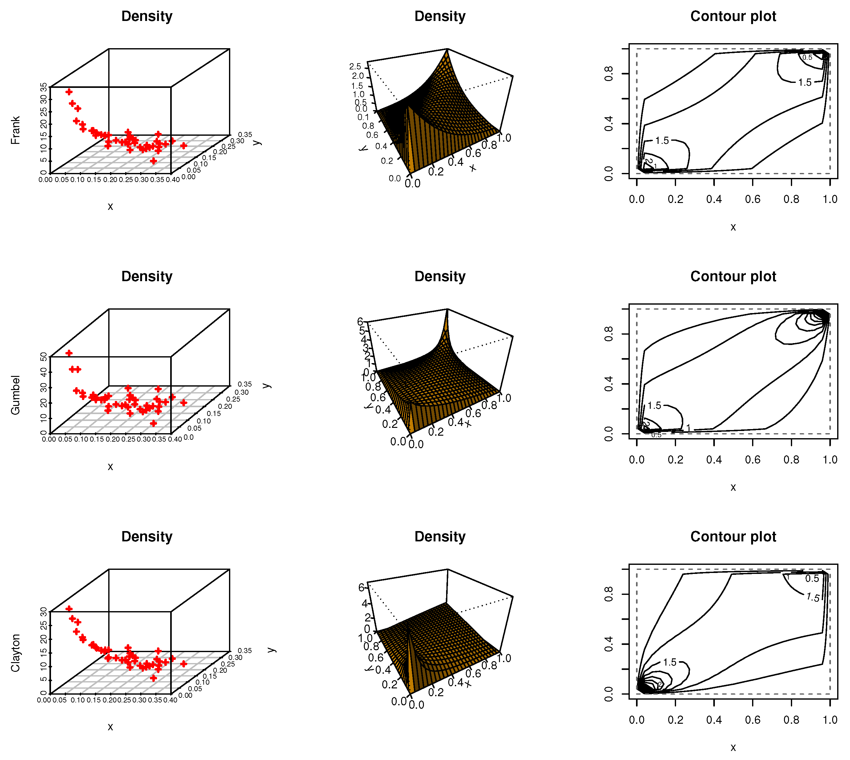
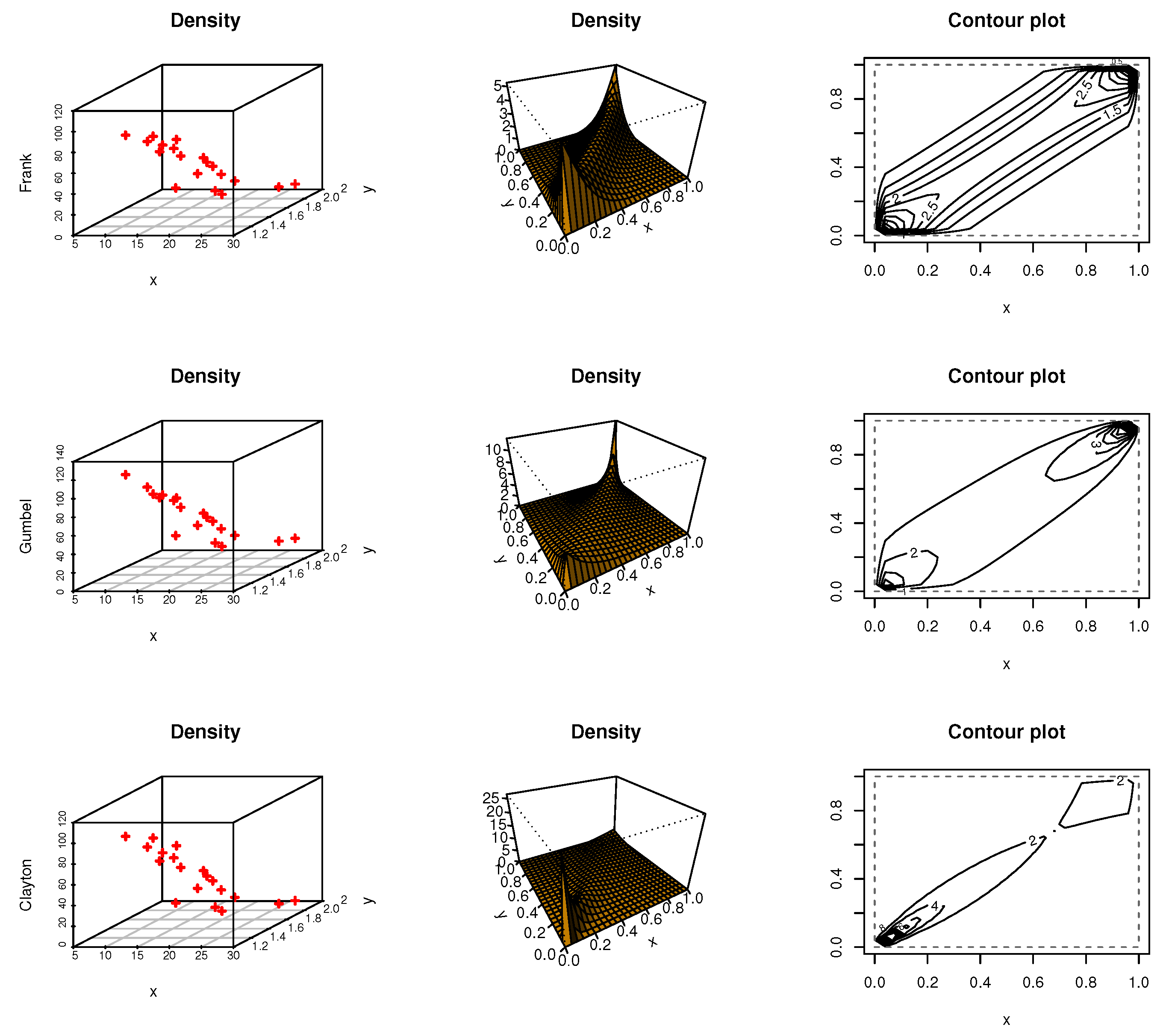
Figure 7 shows the correlation matrix for each dataset, kidney, iron material jobs, and diabetic nephropathy, respectively. All the data under study have a correlation value between 0.04 and 0.16. In addition, Table 5 shows goodness-of-fit measures such as Anderson–Darling (AD), Cramer–von Mises criterion (CVM), and the estimated copula parameter by the non-parametric method to test whether or not these copula are a good fit for this data. By the results of goodness of fit test for each copula, we note that p-values are more than 0.05, then these copula functions are a good fit for these datasets.
Figure 8, Figure 9 and Figure 10 discussed scatter, contour, and density plots for Frank, Gumbel, and Clayton for iron material jobs, diabetic nephropathy, and kidney patients data, respectively.
These included the Akaike information criterion (AIC), the Kolmogorov–Smirnov test, the corrected Akaike information criterion (CAIC), the Bayesian information criterion (BIC), and the Hannan–Quinn information criterion (HQIC). The three real data examples illustrate the suitability of the proposed distributions. Table 6 discussed MLE, StEr, and goodness of fit for different datasets.
Here, we fit the FBXL, CBXL, and GBXL models on each dataset based on Type II censored samples. In Table 7, Table 8 and Table 9, we provide the estimates and Standard Error (StEr) values for all parameters of each model. The Bayesian estimations have smaller StEr than MLE, Therefore, the Bayesian estimation is better than MLE. Also, when r decreases then the StEr of the parameter model increases.

8. Conclusions

In this paper, we introduce the utilization of bivariate models employing copula functions to examine industry data associated with iron material jobs, medical data related to diabetic nephropathy, and the recurrence process of infections among kidney patients. Our analysis of iron material jobs data reveals a significant relationship between the hole diameter and sheet thickness with the size of burrs. Burrs, when present, can adversely impact product performance and reliability by causing friction and wear, potentially leading to premature failure. Hence, it is crucial to manage burr size during the manufacturing process to ensure product quality. Additionally, our investigation into diabetic nephropathy data demonstrates a probabilistic correlation between the duration of diabetes and SrCr levels. Through the analysis of medical data, we establish this relationship in a probabilistic manner. Furthermore, our study of kidney patient data focuses on analyzing infection recurrence times in patients utilizing portable dialysis machines. These empirical findings provide the basis for our approach to the bivariate modeling of iron material jobs, diabetic nephropathy, and infection recurrence processes among kidney patients using various copula functions. Three different copula models were utilized, and their accuracy was assessed by fitting them to real-world data. We have introduced a novel category of BXL distributions derived from Frank, Gumbel, and Clayton copulas. Furthermore, we derived the reliability functions for the BXL distributions, utilizing various copulas under investigation. Consequently, these findings can be effectively applied in life testing data analysis. We employed both the maximum likelihood method and the Bayesian method utilizing the Metropolis–Hastings (M-H) algorithm for parameter estimation, considering both complete and censored samples. Therefore, our findings lead to the conclusion that Bayesian estimation emerges as the optimal estimator for the BXL distribution under various copulas. Monte Carlo simulation was employed to compare distributions, and the results indicate that, in the majority of cases, the bivariate XL based on the Clayton copula outperforms other models. The CBXL distribution has been identified as the most suitable model for fitting the kidney data and iron material jobs, whereas the FBXL distribution demonstrates the best fit for diabetic nephropathy.

Author Contributions

Conceptualization, M.E.Q. and E.M.A.; methodology, A.F., E.M.A. and M.E.Q.; software, E.M.A.; formal analysis, M.E.Q.; writing—original draft, M.E.Q.; writing—review and editing, A.F.; visualization, E.M.A.; project administration, A.F. and M.E.Q.; funding acquisition, A.F. All authors have read and agreed to the published version of the manuscript.

Funding

This research received no external funding.

Data Availability Statement

All data are available in the manuscript.

Conflicts of Interest

The authors declare no conflicts of interest.

Appendix A

By taking partial derivatives of Equation (35) with respect to the parameters of the model, we obtain the following:
F B X L ( φ ) a 1 = 2 n a 1 + i = 1 n 2 + a 1 + x i : n 1 i = 1 n x i : n 2 n 1 + a 1 θ i = 1 n A ( x i : n ) 2 i = 1 n θ A ( x i : n ) e θ u ( x i : n ) 1 e θ v ( y [ i : n ] ) e θ e θ u ( x i : n ) e θ v ( y [ i : n ] ) + e θ u ( x i : n ) + v ( y [ i : n ] ) ,
F B X L ( φ ) a 2 = 2 n a 2 + i = 1 n 2 + a 2 + y [ i : n ] 1 i = 1 n y [ i : n ] 2 n 1 + a 2 θ i = 1 n B ( y [ i : n ] ) 2 i = 1 n θ B ( y [ i : n ] ) e θ v ( y [ i : n ] ) 1 e θ u ( x i : n ) e θ e θ u ( x i : n ) e θ v ( y [ i : n ] ) + e θ u ( x i : n ) + v ( y [ i : n ] ) ,
F B X L ( φ ) θ = n θ i = 1 n u ( x i : n ) + v ( y [ i : n ] ) n e θ e θ 1 2 i = 1 n e θ + u ( x i : n ) e θ u ( x i : n ) + v ( y [ i : n ] ) e θ v ( y [ i : n ] ) u ( x i : n ) + v ( y [ i : n ] ) e θ u ( x i : n ) + v ( y [ i : n ] ) e θ e θ u ( x i : n ) e θ v ( y [ i : n ] ) + e θ u ( x i : n ) + v ( y [ i : n ] ) ,
where
A ( x i : n ) = a 1 u x i : n = x i : n e a 1 x i : n 1 + 1 1 + a 1 2 1 + a 1 x i : n 2 a 1 1 + a 1 ,
and
B ( y [ i : n ] ) = a 2 v y [ i : n ] = y [ i : n ] e a 2 y [ i : n ] 1 + 1 1 + a 2 2 1 + a 2 y [ i : n ] 2 a 2 1 + a 2 .
By taking partial derivatives of Equation (38) with respect to the parameters of the model, we obtain the following:
G B X L ( φ ) a 1 = 2 n a 1 + i = 1 n 2 + a 1 + x i : n 1 i = 1 n x i : n 2 n 1 + a 1 i = 1 n A ( x i : n ) u ( x i : n ) + i = 1 n A ( x i : n ) u ( x i : n ) ln u ( x i : n ) θ 1 ln u ( x i : n ) θ + ln v ( y [ i : n ] ) θ 1 θ 1 + θ 1 i = 1 n A ( x i : n ) u ( x i ) ln u ( x i : n ) + 2 1 θ i = 1 n θ A ( x i : n ) ln u ( x i : n ) θ 1 u ( x i : n ) ln u ( x i : n ) θ + ln v ( y [ i : n ] ) θ i = 1 n θ A ( x i : n ) ln u ( x i : n ) θ 1 u ( x i : n ) ln u ( x i : n ) θ + ln v ( y [ i : n ] ) θ 1 θ + θ 1 ,
G B X L ( φ ) a 2 = 2 n a 2 + i = 1 n 2 + a 2 + y [ i : n ] 1 i = 1 n y [ i : n ] 2 n 1 + a 2 i = 1 n B ( y [ i : n ] ) v ( y [ i : n ] ) + i = 1 n B ( y [ i : n ] ) v ( y i ) ln v ( y [ i : n ] ) θ 1 ln u ( x i : n ) θ + ln v ( y [ i : n ] ) θ 1 θ 1 + θ 1 i = 1 n B ( y [ i : n ] ) v ( y i ) ln v ( y [ i : n ] ) + 2 1 θ i = 1 n θ B ( y [ i : n ] ) ln v ( y [ i : n ] ) θ 1 u ( x i : n ) ln u ( x i : n ) θ + ln v ( y [ i : n ] ) θ i = 1 n θ B ( y [ i : n ] ) ln v ( y [ i : n ] ) θ 1 v ( y [ i : n ] ) ln u ( x i : n ) θ + ln v ( y [ i : n ] ) θ 1 θ + θ 1 ,
G B X L ( φ ) θ = i = 1 n G ( x i : n , y [ i : n ] ) + i = 1 n ln ln u ( x i : n ) + ln ln v ( y [ i : n ] ) + 1 θ i = 1 n ln u ( x i : n ) θ ln ln u ( x i : n ) + ln v ( y [ i : n ] ) θ ln ln v ( y [ i : n ] ) ln u ( x i : n ) θ + ln v ( y [ i : n ] ) θ 1 θ 2 i = 1 n ln ln u ( x i : n ) θ + ln v ( y [ i : n ] ) θ + i = 1 n G ( x i : n , y [ i : n ] ) + 1 ln u ( x i : n ) θ + ln v ( y [ i : n ] ) θ 1 θ + θ 1 ,
where
G ( x i : n , y [ i : n ] ) = θ ln u ( x i : n ) θ + ln v ( y [ i : n ] ) θ 1 θ = 1 θ ln u ( x i : n ) θ ln ln u ( x i : n ) + ln v ( y [ i : n ] ) θ ln ln v ( y [ i : n ] ) ln u ( x i : n ) θ + ln v ( y [ i : n ] ) θ 1 θ 1
By taking partial derivatives of Equation (39) with respect to the parameters of the model, we obtain the following:
C B X L ( φ ) a 1 = 2 n a 1 + i = 1 n 2 + a 1 + x i : n 1 i = 1 n x i : n 2 n 1 + a 1 1 + θ i = 1 n A ( x i : n ) u x i : n + 2 + 1 θ i = 1 n θ A ( x i : n ) u ( x i : n ) θ 1 u ( x i : n ) θ + v ( y [ i : n ] ) θ 1 ,
C B X L ( φ ) a 2 = 2 n a 2 + i = 1 n 2 + a 2 + y [ i : n ] 1 i = 1 n y [ i : n ] 2 n 1 + a 2 1 + θ i = 1 n B ( y [ i : n ] ) v y [ i : n ] + 2 + 1 θ i = 1 n θ B ( y [ i : n ] ) v ( y [ i : n ] ) θ 1 u ( x i : n ) θ + v ( y [ i : n ] ) θ 1 ,
C B X L ( φ ) θ = n 1 + θ i = 1 n ln u ( x i : n ) + ln v ( y [ i : n ] ) + 1 θ 2 i = 1 n ln u ( x i : n ) θ + v ( y [ i : n ] ) θ 1 + 1 θ i = 1 n u ( x i : n ) θ ln u ( x i : n ) + v ( y [ i : n ] ) θ ln v ( y [ i : n ] ) u ( x i : n ) θ + v ( y [ i : n ] ) θ 1 ,

Appendix B

By taking partial derivatives of Equation (42) with respect to the parameters of the model, we obtain the following:
F B X L C ( φ ) a 1 = ( n r ) D ( x r : n ) x r : n + 2 n a 1 + i = 1 r 2 + a 1 + x i : n 1 i = 1 r x i : n 2 n 1 + a 1 θ i = 1 r A ( x i : n ) 2 i = 1 r θ A e θ u ( x i : n ) 1 e θ v ( y [ i : n ] ) e θ e θ u ( x i : n ) e θ v ( y [ i : n ] ) + e θ u ( x i : n ) + v ( y [ i : n ] ) ,
F B X L C ( φ ) a 2 = 2 n a 2 + i = 1 r 2 + a 2 + y [ i : n ] 1 i = 1 r y [ i : n ] 2 n 1 + a 2 θ i = 1 r B ( y [ i : n ] ) 2 i = 1 r θ B e θ v ( y [ i : n ] ) 1 e θ u ( x i : n ) e θ e θ u ( x i : n ) e θ v ( y [ i : n ] ) + e θ u ( x i : n ) + v ( y [ i : n ] ) ,
F B X L C ( φ ) θ = n θ i = 1 r u ( x i : n ) + v ( y [ i : n ] ) n e θ e θ 1 2 i = 1 r e θ + u ( x i : n ) e θ u ( x i : n ) + v ( y [ i : n ] ) e θ v ( y [ i : n ] ) u ( x i : n ) + v ( y [ i : n ] ) e θ u ( x i : n ) + v ( y [ i : n ] ) e θ e θ u ( x i : n ) e θ v ( y [ i : n ] ) + e θ u ( x i : n ) + v ( y [ i : n ] ) ,
where
D ( x r : n ) = a 1 ln 1 + a 1 x r : n 1 + a 1 2 = x r : n 1 a 1 1 a 1 1 a 1 2 + a 1 x r : n ,
By taking partial derivatives of Equation (45) with respect to the parameters of the model, we obtain the following:
G B X L C ( φ ) a 1 = ( n r ) D ( x r : n ) x r : n + 2 n a 1 + i = 1 r 2 + a 1 + x i : n 1 i = 1 r x i : n 2 n 1 + a 1 i = 1 r A ( x i : n ) u ( x i : n ) + i = 1 r A ( x i : n ) u ( x i : n ) ln u ( x i : n ) θ 1 ln u ( x i : n ) θ + ln v ( y [ i : n ] ) θ 1 θ 1 + θ 1 i = 1 r A ( x i : n ) u ( x i : n ) ln u ( x i : n ) + 2 1 θ i = 1 r θ A ( x i : n ) ln u ( x i : n ) θ 1 u ( x i : n ) ln u ( x i : n ) θ + ln v ( y [ i : n ] ) θ i = 1 r θ A ( x i : n ) ln u ( x i : n ) θ 1 u ( x i : n ) ln u ( x i : n ) θ + ln v ( y [ i : n ] ) θ 1 θ + θ 1 ,
G B X L C ( φ ) a 2 = 2 n a 2 + i = 1 r 2 + a 2 + y [ i : n ] 1 i = 1 r y [ i : n ] 2 n 1 + a 2 i = 1 r B ( y [ i : n ] ) v ( y i : n ) + i = 1 r B ( y [ i : n ] ) v ( y [ i : n ] ) ln v ( y [ i : n ] ) θ 1 ln u ( x i : n ) θ + ln v ( y [ i : n ] ) θ 1 θ 1 + θ 1 i = 1 r B ( y [ i : n ] ) v ( y [ i : n ] ) ln v ( y [ i : n ] ) + 2 1 θ i = 1 r θ B ( y [ i : n ] ) ln v ( y [ i : n ] ) θ 1 u ( x i : n ) ln u ( x i : n ) θ + ln v ( y [ i : n ] ) θ i = 1 r θ B ( y [ i : n ] ) ln v ( y [ i : n ] ) θ 1 v ( y [ i : n ] ) ln u ( x i : n ) θ + ln v ( y [ i : n ] ) θ 1 θ + θ 1 ,
G B X L C ( φ ) θ = i = 1 r G ( x i : n , y [ i : n ] ) + i = 1 r ln ln u ( x i : n ) + ln ln v ( y [ i : n ] ) + 1 θ i = 1 r ln u ( x i : n ) θ ln ln u ( x i : n ) + ln v ( y [ i : n ] ) θ ln ln v ( y [ i : n ] ) ln u ( x i : n ) θ + ln v ( y [ i : n ] ) θ 1 θ 2 i = 1 r ln ln u ( x i : n ) θ + ln v ( y [ i : n ] ) θ + i = 1 r G ( x i : n , y [ i : n ] ) + 1 ln u ( x i : n ) θ + ln v ( y [ i : n ] ) θ 1 θ + θ 1 ,
where
G ( x i : n , y [ i : n ] ) = θ ln u ( x i : n ) θ + ln v ( y [ i : n ] ) θ 1 θ = 1 θ ln u ( x i : n ) θ ln ln u ( x i : n ) + ln v ( y [ i : n ] ) θ ln ln v ( y [ i : n ] ) ln u ( x i : n ) θ + ln v ( y [ i : n ] ) θ 1 θ 1
By taking partial derivatives of Equation (46) with respect to the parameters of the model, we obtain the following:
C B X L C ( φ ) a 1 = ( n r ) D ( x r : n ) x r : n + 2 n a 1 + i = 1 r 2 + a 1 + x i : n 1 i = 1 r x i 2 n 1 + a 1 1 + θ i = 1 r A ( x i : n ) u x i : n + 2 + 1 θ i = 1 r θ A ( x i : n ) u ( x i : n ) θ 1 u ( x i : n ) θ + v ( y [ i : n ] ) θ 1 ,
C B X L C ( φ ) a 2 = 2 n a 2 + i = 1 r 2 + a 2 + y [ i : n ] 1 i = 1 r y [ i : n ] 2 n 1 + a 2 1 + θ i = 1 r B ( y [ i : n ] ) v y [ i : n ] + 2 + 1 θ i = 1 r θ B ( y [ i : n ] ) v ( y [ i : n ] ) θ 1 u ( x i : n ) θ + v ( y [ i : n ] ) θ 1 ,
C B X L C ( φ ) θ = n 1 + θ i = 1 r ln u ( x i : n ) + ln v ( y [ i : n ] ) + 1 θ 2 i = 1 r ln u ( x i : n ) θ + v ( y [ i : n ] ) θ 1 + 1 θ i = 1 n u ( x i : n ) θ ln u ( x i : n ) + v ( y [ i : n ] ) θ ln v ( y [ i : n ] ) u ( x i : n ) θ + v ( y [ i : n ] ) θ 1 ,

References

  1. Ashkar, F.; Aucoin, F. Bivariate Models Constructed by the Marginal Transformation Method: With Applications in Hydrology. In Proceedings of the World Environmental and Water Resources Congress 2010: Challenges of Change, Providence, RI, USA, 16 May 2010; American Society of Civil Engineers: Reston, VA, USA, 2010; pp. 2467–2477. [Google Scholar]
  2. Nelsen, R.B. An Introduction to Copulas; Springer: Berlin/Heidelberg, Germany, 2007; ISBN 978-0387286594. [Google Scholar]
  3. Arnold, B.C.; Sarabia, J.M. Conditional specification of statistical models: Classical models, new developments and challenges. J. Multivar. Anal. 2022, 188, 104801. [Google Scholar] [CrossRef]
  4. Vincent Raja, A.; Gopalakrishnan, A. On the Analysis of Bivariate Lifetime Data: Some Models and Applications. Ph.D. Thesis, Cochin University of Science and Technology, Kochi, India, 2017. [Google Scholar]
  5. Marshall, A.W.; Olkin, I.A. Multivariate exponential model. J. Am. Stat. Assoc. 1967, 62, 30–44. [Google Scholar] [CrossRef]
  6. Pathak, A.K.; Vellaisamy, P. A bivariate generalized linear exponential distribution: Properties and estimation. Commun. -Stat.-Simul. Comput. 2022, 51, 5426–5446. [Google Scholar] [CrossRef]
  7. Ghosh, I.; Watts, D.; Chakraborty, S. Modeling Bivariate Dependency in Insurance Data via Copula: A Brief Study. J. Risk Financ. Manag. 2022, 15, 329. [Google Scholar] [CrossRef]
  8. Frees, E.W.; Valdez, E.A. Understanding relationships using copulas. N. Am. Actuar. J. 1998, 2, 1–25. [Google Scholar] [CrossRef]
  9. Otani, Y.; Imai, J. Pricing Portfolio Credit Derivatives with Stochastic Recovery and Systematic Factor. IAENG Int. J. Appl. Math. 2013, 43, 176–184. [Google Scholar]
  10. Nikoloulopoulos, A.K.; Joe, H.; Li, H. Vine copulas with asymmetric tail dependence and applications to financial return data. Comput. Stat. Data Anal. 2012, 56, 3659–3673. [Google Scholar] [CrossRef]
  11. Genest, C.; Nešlehová, J.; Quessy, J.F. Tests of symmetry for bivariate copulas. Ann. Inst. Stat. Math. 2012, 64, 811–834. [Google Scholar] [CrossRef]
  12. Winkelmann, R. Copula bivariate probit models: With an application to medical expenditures. Health Econ. 2012, 21, 1444–1455. [Google Scholar] [CrossRef]
  13. Flores, A.Q. Testing copula functions as a method to derive bivariate Weibull distributions. In Proceedings of the American Political Science Association (APSA), Annual Meeting, Toronto, ON, Canada, 3–6 September 2009; pp. 1–19. [Google Scholar]
  14. Abd Elaal, M.K.; Jarwan, R.S. Inference of bivariate generalized exponential distribution based on copula functions. Appl. Math. Sci. 2017, 11, 1155–1186. [Google Scholar]
  15. Baharith, L.; Alzahrani, H. New bivariate Pareto type II models. Entropy 2019, 21, 473. [Google Scholar] [CrossRef]
  16. El-Sherpieny, E.S.A.; Almetwally, E.M.; Muhammed, H.Z. Bayesian and non-bayesian estimation for the parameter of bivariate generalized Rayleigh distribution based on clayton copula under progressive Type II censoring with random removal. Sankhya A 2021, 85, 1–38. [Google Scholar] [CrossRef]
  17. Usman, U.; Aliyu, Y. Bivariate Nadarajah-Haghighi distribution derived from copula functions: Bayesian estimation and applications. Benin J. Stat. 2022, 5, 45. [Google Scholar]
  18. Qura, M.E.; Fayomi, A.; Kilai, M.; Almetwally, E.M. Bivariate power Lomax distribution with medical applications. PLoS ONE 2023, 18, e0282581. [Google Scholar] [CrossRef]
  19. Fayomi, A.; Almetwally, E.M.; Qura, M.E. A novel bivariate Lomax-G family of distributions: Properties, inference, and applications to environmental, medical, and computer science data. AIMS Math. 2023, 8, 17539–17584. [Google Scholar] [CrossRef]
  20. Fayomi, A.; Almetwally, E.M.; Qura, M.E. Exploring New Horizons: Advancing Data Analysis in Kidney Patient Infection Rates and UEFA Champions League Scores Using Bivariate Kavya–Manoharan Transformation Family of Distributions. Mathematics 2023, 11, 2986. [Google Scholar] [CrossRef]
  21. Balakrishnan, N.; Kim, J.A. EM Algorithm for Type-II Right Censored Bivariate Normal Data. In Parametric and Semiparametric Models with Applications to Reliability, Survival Analysis, and Quality of Life; Balakrishnan, N., Nikulin, M.S., Mesbah, M., Limnios, N., Eds.; Birkhäuser: Basel, Switzerland, 2004; pp. 177–210. [Google Scholar]
  22. Kim, S.W.; Ng, H.K.T.; Jang, H. Estimation of parameters in a bivariate generalized exponential distribution based on Type-II censored samples. Commun.-Stat.-Simul. Comput. 2016, 45, 3776–3797. [Google Scholar] [CrossRef]
  23. Almetwally, E.M. Parameter Estimation of Bivariate Models under Some Censoring Schemes; Cairo University: Giza, Egypt, 2019. [Google Scholar]
  24. Bai, X.; Shi, Y.; Liu, B.; Fu, Q. Statistical inference of Marshall-Olkin bivariate Weibull distribution with three shocks based on progressive interval censored data. Commun.-Stat.-Simul. Comput. 2019, 48, 637–654. [Google Scholar] [CrossRef]
  25. El-Morshedy, M.; Alhussain, Z.A.; Atta, D.; Almetwally, E.M.; Eliwa, M.S. Bivariate Burr X generator of distributions: Properties and estimation methods with applications to complete and type-II censored samples. Mathematics 2020, 8, 264. [Google Scholar] [CrossRef]
  26. Lin, Y.H.; Sun, L.H.; Tseng, Y.J.; Emura, T. The Pareto type I joint frailty-copula model for clustered bivariate survival data. Commun.-Stat.-Simul. Comput. 2022, 53, 2006–2030. [Google Scholar] [CrossRef]
  27. Haj Ahmad, H.; Almetwally, E.M.; Ramadan, D.A. Investigating the Relationship between Processor and Memory Reliability in Data Science: A Bivariate Model Approach. Mathematics 2023, 11, 2142. [Google Scholar] [CrossRef]
  28. Gramaje, A.; Thabtah, F.; Abdelhamid, N.; Ray, S.K. Patient discharge classification using machine learning techniques. Ann. Data Sci. 2021, 8, 755–767. [Google Scholar] [CrossRef]
  29. Tien, J.M. Internet of things, real-time decision making, and artificial intelligence. Ann. Data Sci. 2017, 4, 149–178. [Google Scholar] [CrossRef]
  30. Chouia, S.; Zeghdoudi, H. The XLindley distribution: Properties and application. J. Stat. Theory Appl. 2021, 20, 318–327. [Google Scholar] [CrossRef]
  31. Ahsan-ul-Haq, M.; Al-Bossly, A.; El-Morshedy, M.; Eliwa, M.S. Poisson XLindley distribution for count data: Statistical and reliability properties with estimation techniques and inference. Comput. Intell. Neurosci. 2022, 2022, 6503670. [Google Scholar] [CrossRef]
  32. Etaga, H.O.; Nwankwo, M.P.; Oramulu, D.O.; Anabike, I.C.; Obulezi, O.J. The Double XLindley Distribution: Properties and Applications. Sch. J. Phys. Math. Stat. 2023, 10, 192–202. [Google Scholar] [CrossRef]
  33. Musekwa, R.R.; Makubate, B. A flexible generalized XLindley distribution with application to engineering. Sci. Afr. 2024, 24, e02192. [Google Scholar] [CrossRef]
  34. Gemeay, A.M.; Beghriche, A.; Sapkota, L.P.; Zeghdoudi, H.; Makumi, N.; Bakr, M.E.; Balogun, O.S. Modified XLindley distribution: Properties, estimation, and applications. AIP Adv. 2023, 13, e095021. [Google Scholar] [CrossRef]
  35. Alotaibi, R.; Nassar, M.; Elshahhat, A. Computational Analysis of XLindley Parameters Using Adaptive Type-II Progressive Hybrid Censoring with Applications in Chemical Engineering. Mathematics 2022, 10, 3355. [Google Scholar] [CrossRef]
  36. Alotaibi, R.; Nassar, M.; Elshahhat, A. Reliability Estimation under Normal Operating Conditions for Progressively Type-II XLindley Censored Data. Axioms 2023, 12, 352. [Google Scholar] [CrossRef]
  37. Sklar, M. Fonctions de répartition à n dimensions et leurs marges. Annales de l’ISUP 1959, 8, 229–231. [Google Scholar]
  38. Joe, H. Dependence Modeling with Copulas; CRC Press: New York, NY, USA, 2014. [Google Scholar]
  39. Frank, M.J. On the simultaneous associativity of F(x; y) and x + yF(x; y). Aequationes Math. 1979, 99, 194–226. [Google Scholar] [CrossRef]
  40. Nelsen, R.B. Properties of a one-parameter family of bivariate distributions with specified marginals. Commun.-Stat.-Theory Methods 1986, 15, 3277–3285. [Google Scholar] [CrossRef]
  41. Genest, C. Frank’s family of bivariate distributions. Biometrika 1987, 74, 549–555. [Google Scholar] [CrossRef]
  42. Gumbel, E.J. Distributions des Valeurs Extrêmes en Plusieurs Dimensions; Publications de l’Institut de Statistique de l’Université de Paris: Paris, France, 1960; Volume 9, pp. 171–173. [Google Scholar]
  43. Hougaard, P. A class of multivanate failure time distributions. Biometrika 1986, 73, 671–678. [Google Scholar] [CrossRef]
  44. Hutchinson, T.P.; Lai, C.D. Continuous Bivariate Distributions Emphasising Applications; Rumsby Scientific Publishing: Adelaide, Australia, 1990. [Google Scholar]
  45. Clayton, D.G. A model for association in bivariate life tables and its application in epidemiological studies of familial tendency in chronic disease incidence. Biometrika 1978, 65, 141–151. [Google Scholar] [CrossRef]
  46. Cook, R.D.; Johnson, M.E. A family of distributions for modelling non-elliptically symmetric multivariate data. J. R. Stat. Soc. Ser. Stat. Methodol. 1981, 43, 210–218. [Google Scholar] [CrossRef]
  47. Oakes, D. A model for association in bivariate survival data. J. R. Stat. Soc. Ser. Stat. Methodol. 1982, 44, 414–422. [Google Scholar] [CrossRef]
  48. Basu, A.P. Bivariate failure rate. J. Am. Stat. Assoc. 1971, 66, 103–104. [Google Scholar] [CrossRef]
  49. David, H.A.; Nagaraja, H.N. Order Statistics, 2nd ed.; Wiley: New York, NY, USA, 2003. [Google Scholar]
  50. Kim, G.; Silvapulle, M.J.; Silvapulle, P. Comparison of semiparametric and parametric methods for estimating copulas. Comput. Stat. Data Anal. 2007, 51, 2836–2850. [Google Scholar] [CrossRef]
  51. Muhammed, H.Z.; Almetwally, E.M. Bayesian and non-Bayesian estimation for the bivariate inverse Weibull distribution under progressive type-II censoring. Ann. Data Sci. 2023, 10, 481–512. [Google Scholar] [CrossRef]
  52. Chen, M.H.; Shao, Q.M. Monte Carlo estimation of Bayesian credible and HPD intervals. J. Comput. Graph. Stat. 1999, 8, 69–92. [Google Scholar] [CrossRef]
  53. Dasgupta, R. On the distribution of burr with applications. Sankhya B 2011, 73, 1–19. [Google Scholar] [CrossRef]
  54. Skrotzki, W.; Kegler, K.; Tamm, R.; Oertel, C.G. Grain structure and texture of cast iron aluminides. Cryst. Res. Technol. J. Exp. Ind. Crystallogr. 2005, 40, 90–94. [Google Scholar] [CrossRef]
  55. Grover, G.; Sabharwal, A.; Mittal, J. Application of multivariate and bivariate normal distributions to estimate duration of diabetes. Int. J. Stat. Appl. 2014, 4, 46–57. [Google Scholar]
  56. McGilchrist, C.A.; Aisbett, C.W. Regression with frailty in survival analysis. Biometrics 1991, 47, 461–466. [Google Scholar] [CrossRef]
Figure 1. Plots of joint density FBXL distribution for some parameter values.
Mathematics 12 01774 g001
Figure 2. Plots of hazard rate function of the FBXL distribution for some parameter values.
Mathematics 12 01774 g002
Figure 3. Plots of joint density GBXL distribution for some parameter values.
Mathematics 12 01774 g003
Figure 4. Plots of hazard rate function of the GBXL distribution for some parameter values.
Mathematics 12 01774 g004
Figure 5. Plots of joint density CBXL distribution for some parameter values.
Mathematics 12 01774 g005
Figure 6. Plots of hazard rate function of the CBXL distribution for some parameter values.
Mathematics 12 01774 g006
Figure 7. Correlation matrix for each dataset.
Mathematics 12 01774 g007
Figure 8. Scatter, contour, and density plots for Frank, Gumbel, and Clayton with iron material jobs data.
Mathematics 12 01774 g008
Figure 9. Scatter, contour, and density plots for Frank, Gumbel, and Clayton with diabetic nephropathy data.
Mathematics 12 01774 g009
Figure 10. Scatter, contour, and density plots for Frank, Gumbel, and Clayton with kidney patients data.
Mathematics 12 01774 g010
Table 1. MB, MSE, and LACI for MLE and Bayesian based on TIICS for Frank, Clayton, and Gumbel copula: a 1 = 2 , a 2 = 2 , θ = 1.5 .
MLEBayesian
FrankClaytonGumbelFrankClaytonGumbel
nr MBMSELACICPMBMSELACICPMBMSELACICPMBMSELCCIMBMSELCCIMBMSELCCI
3525 a 1 0.41230.27761.286593.40%−0.06210.07221.025394.50%1.94134.45893.258994.65%0.01840.00200.1555−0.02060.00250.17490.03280.00270.1502
a 2 0.40810.27251.276695.13%−0.06660.06820.990594.67%2.72518.37653.823294.60%0.02270.00110.08590.00970.00090.10230.16280.02750.1144
θ 1.75674.44404.570694.17%−0.78391.39463.464294.13%−0.01040.04230.805694.00%0.22740.46612.3989−0.67780.67231.43760.31900.22791.2894
τ 0.15790.03390.370794.00%−0.21320.07320.653094.65%−0.28410.08980.373394.75%0.02140.00460.1555−0.15360.03410.1749−0.17070.04140.1502
ρ 0.22080.06520.502695.33%−0.29250.13550.876794.77%−0.33870.13110.502694.96%0.03020.00950.0859−0.20310.06000.1023−0.19630.05740.1144
32 a 1 0.39570.20430.856394.67%−0.08090.03840.699894.67%1.87753.91742.456195.33%0.01480.00110.1106−0.00030.00120.13410.02330.00160.1162
a 2 0.39780.21260.914695.00%−0.08090.04300.749196.33%2.63157.42472.772796.97%0.01240.00050.07300.00230.00050.08390.10010.01060.0940
θ 1.62283.24583.069295.67%−0.96791.13921.764095.00%−0.05220.02610.599695.30%0.03470.14101.3746−0.35650.25691.27520.19000.09180.8801
τ 0.15100.02720.261394.87%−0.23860.07070.460294.97%−0.26990.08200.315797.33%0.00300.00150.1106−0.07300.01060.1341−0.16200.04090.1162
ρ 0.21340.05390.358495.30%−0.32260.13060.638696.73%−0.35770.12400.432996.67%0.00410.00320.0730−0.09390.01760.0839−0.18230.05470.0940
35 a 1 0.37750.16500.589195.97%−0.09510.02430.484896.33%1.71633.29322.312294.00%0.01470.00100.1058−0.00020.00110.13060.00890.00140.1055
a 2 0.37830.16820.622095.17%−0.09370.02630.519895.93%2.42596.36862.727595.67%0.00690.00040.07290.00220.00040.10210.06060.00440.1078
θ 1.57512.76282.082495.50%−1.03981.14180.966496.97%−0.06690.01750.448093.67%0.02070.02840.6143−0.07360.04020.69120.07660.02830.5833
τ 0.14890.02430.179596.67%−0.24920.06810.303596.93%−0.30250.08100.235694.00%0.00200.00030.1576−0.01400.00120.1358−0.14030.04060.1549
ρ 0.21160.04870.246796.67%−0.33470.12420.432996.83%−0.32610.11370.319895.67%0.00290.00070.0920−0.01750.00190.1021−0.17960.04850.1078
10070 a 1 0.21100.17481.417695.33%−0.17760.14681.333495.00%1.74525.99986.751594.33%0.03060.00320.1823−0.05890.00610.20810.09300.01130.2049
a 2 0.21340.17551.416195.27%−0.18890.13401.231594.33%2.77047.29516.358294.37%0.05750.00410.10500.02830.00190.12220.41380.17260.1443
θ 1.45962.22472.036295.67%−0.86741.58502.079895.33%−0.22673.06486.818894.80%0.32900.47402.1841−1.00541.09580.79880.17500.07550.8011
τ 0.14200.03250.278796.33%−0.57250.35240.616895.20%−0.20310.09320.895396.33%0.03190.00470.1823−0.23900.06290.2081−0.20660.04860.2049
ρ 0.21520.06470.320695.47%−0.74750.60860.876895.33%−0.21240.12101.081994.67%0.04570.00990.1050−0.32030.11370.1222−0.23740.06600.1443
85 a 1 0.20810.09550.899796.33%−0.20360.07140.681296.33%1.51594.62636.009896.00%0.02800.00190.1292−0.02780.00210.14100.05650.00460.1400
a 2 0.16740.08280.921796.43%−0.21070.09370.874996.33%2.37436.70964.078796.53%0.03380.00160.08240.00540.00060.08830.24470.06070.1174
θ 1.31932.00142.015595.60%−0.92511.46080.891996.33%−0.85491.62543.725197.00%0.12370.13951.3874−0.64800.52851.14960.16230.06360.7992
τ 0.13990.03040.190696.63%−0.57470.34040.395596.53%−0.19330.09181.057696.60%0.01220.00140.1292−0.13870.02520.1410−0.18630.03960.1400
ρ 0.20520.06060.219496.73%−0.74900.58300.584096.73%−0.23620.10241.003396.73%0.01760.00310.0824−0.18080.04340.0883−0.21150.05250.1174
100 a 1 0.21140.05780.467896.90%−0.19530.04310.287396.67%0.82091.37073.417897.50%0.02780.00180.1636−0.00590.00190.16670.04090.00350.1572
a 2 0.18400.04560.443397.67%−0.21430.05950.476796.85%1.67643.58653.607496.83%0.02070.00130.1138−0.00160.00050.08010.16210.02730.1282
θ 1.07181.98902.090897.67%−0.79901.39520.429697.67%−0.72011.59632.956097.67%0.06230.03550.6594−0.18770.06720.68740.14710.04040.4827
τ 0.18930.03020.152397.60%−0.55980.33600.211397.67%−0.17970.08210.968797.85%0.00630.00040.1636−0.03420.00230.1667−0.17210.03470.1357
ρ 0.24090.05980.172297.97%−0.70830.56190.316296.95%−0.21440.10030.952497.33%0.00920.00080.1138−0.04250.00350.1017−0.20420.05060.1028
Table 2. MB, MSE, and LACI for MLE and Bayesian based on TIICS for Frank, Clayton, and Gumbel copula: a 1 = 0.5 , a 2 = 1.5 , θ = 2 .
MLEBayesian
Frank ClaytonGumbelFrankClaytonGumbel
nr MBMSELACICPMBMSELACICPMBMSELACICPMBMSELACIMBMSELACIMBMSELACI
3525 a 1 0.06570.01220.348793.50%−0.07170.01000.272694.50%0.20220.11051.034694.60%0.03350.00430.2303−0.03150.00400.21620.06340.01060.2922
a 2 0.43600.45702.026295.03%0.22810.19121.463295.33%5.305140.231713.635494.56%0.03560.00190.0966−0.00010.00110.12160.20310.04300.1593
θ 1.60946.56087.815193.33%−2.03174.28791.570094.33%0.58453.59077.069394.58%0.09120.44452.3307−1.13661.46191.53290.17680.35842.0608
τ 0.12180.03880.606894.50%−0.54570.32130.601695.00%−0.10560.02250.418595.16%0.00660.00410.2303−0.21100.05230.2162−0.16000.04400.2922
ρ 0.16050.06950.820895.33%−0.75070.61240.866395.43%−0.10930.02120.376395.04%0.00830.00830.0966−0.26710.08480.1216−0.17080.05430.1593
32 a 1 0.07040.01040.288894.67%−0.04910.00580.229995.67%0.19480.10710.913594.83%0.03180.00220.1321−0.00810.00170.16160.04890.00520.2047
a 2 0.31620.18561.147795.00%−0.03270.05910.944496.00%3.077915.56399.679095.33%0.02030.00090.0836−0.00110.00060.09000.13200.01830.1106
θ 1.83635.32565.482096.33%−1.84653.60261.722995.63%0.28900.74603.192395.30%0.12360.15741.4883−0.63630.55751.46060.14330.16281.4535
τ 0.15030.03370.412994.97%−0.45860.23440.608695.77%−0.09930.02130.406595.83%0.01140.00150.1321−0.10230.01500.1616−0.14850.03000.2047
ρ 0.20340.06090.547496.25%−0.62300.43810.876396.90%−0.14650.02040.350796.53%0.01600.00300.0836−0.12440.02250.0900−0.15130.03330.1106
35 a 1 0.07460.01010.277496.44%−0.04160.00460.205696.14%0.18350.09170.840496.00%0.03030.00200.13090.00070.00160.15900.02750.00380.2283
a 2 0.25680.12450.948996.47%−0.11850.05540.797695.90%1.92934.62063.717897.33%0.01310.00080.0750−0.00080.00060.08800.07980.00720.1121
θ 1.62304.55024.926996.53%−1.72613.21001.883597.17%−0.04280.33732.271696.67%0.02220.02880.6094−0.14490.05510.7166−0.00850.03880.7459
τ 0.14820.03090.345996.57%−0.41040.19200.602597.40%−0.08180.02070.400696.90%0.00200.00030.1391−0.02000.00100.1901−0.13900.02980.2003
ρ 0.20050.06010.445996.75%−0.55310.35410.860796.50%−0.13940.02090.318797.53%0.00290.00060.1075−0.02330.00140.1088−0.13760.03150.1102
10070 a 1 0.05810.00610.203194.57%−0.08270.00810.139694.38%0.13430.06690.867095.33%0.03440.00250.1308−0.05890.00430.10990.10420.01370.2101
a 2 0.37800.23001.157994.53%0.18930.08290.850794.33%5.566138.695210.893095.62%0.08000.00740.12500.01450.00180.15580.46400.21830.2119
θ 1.35103.11664.456894.67%−2.08704.38000.612694.33%0.16640.23021.765194.33%0.38820.50492.1920−1.53692.39080.53950.30380.44122.1553
τ 0.11530.02180.361494.70%−0.55180.31070.309194.83%−0.14120.02410.252795.65%0.03560.00440.1308−0.31540.10200.1099−0.12990.03100.2101
ρ 0.15820.04060.489495.33%−0.75980.59090.456494.93%−0.14050.02370.248296.17%0.05000.00880.1250−0.41030.17340.1558−0.13570.03590.2119
85 a 1 0.05330.00470.170696.00%−0.06910.00600.137095.67%0.25210.13291.032895.80%0.03440.00220.1245−0.03370.00210.12380.08890.01000.1804
a 2 0.28930.12310.778095.67%−0.01190.02730.646595.67%3.469517.64709.288796.00%0.04750.00280.0868−0.00990.00090.10860.30470.09450.1472
θ 1.06292.93733.330295.67%−1.97543.93440.703695.46%0.16150.19751.624196.67%0.18410.16461.3594−1.15751.39080.83090.25630.18821.4448
τ 0.14120.02440.261096.50%−0.49520.25210.326896.67%−0.14370.02690.309896.80%0.01730.00150.1245−0.20780.04600.1238−0.12180.02120.1804
ρ 0.19470.04580.347995.97%−0.67570.47180.485096.67%−0.14470.02840.338996.80%0.02450.00310.0868−0.26040.07280.1086−0.12100.02290.1472
100 a 1 0.06830.00620.155796.00%−0.05450.00440.146295.80%0.33160.13640.638096.84%0.03040.00200.0961−0.01440.00130.13020.04810.00370.1432
a 2 0.24240.07730.533496.84%−0.10430.02730.508396.95%1.76363.26771.556097.37%0.02390.00120.0998−0.00760.00080.10020.21490.04730.1190
θ 2.06314.70392.624296.67%−1.83313.39300.711296.93%−0.25610.22181.550197.16%0.03860.02960.6280−0.36340.15920.61190.00440.02830.5686
τ 0.17620.03340.191796.90%−0.42900.18940.287197.50%−0.27300.09770.597197.43%0.00370.00030.0961−0.05110.00320.1302−0.11690.02030.1432
ρ 0.24160.06240.248397.43%−0.57730.34500.423997.85%−0.30490.13300.784697.47%0.00520.00060.0998−0.05990.00450.1178−0.10700.02030.1019
Table 3. MB, MSE, and LACI for MLE and Bayesian based on TIICS for Frank, Clayton, and Gumbel copula: a 1 = 3 , a 2 = 1.5 , θ = 2 .
MLEBayesian
Frank ClaytonGumbelFrankClaytonGumbel
nr MBMSELACICPMBMSELACICPMBMSELACICPMBMSELACIMBMSELACIMBMSELACI
3525 a 1 0.52210.78512.807794.50%−0.18790.54122.789595.00%0.59281.78174.690493.67%0.01190.00150.1448−0.01850.00190.15500.02950.00300.1864
a 2 0.43230.45362.025494.53%0.32070.28851.689792.67%5.683733.224712.287894.67%0.03480.00190.09450.00700.00150.14810.19550.04100.2119
θ 1.61366.58997.830494.57%−1.93324.07262.271895.17%0.23861.17624.149394.63%0.20290.48242.5531−1.10361.41931.60750.19070.40392.1943
τ 0.12210.03890.607295.10%−0.51120.29030.667295.60%−0.14480.02660.293195.37%0.01740.00430.1448−0.20450.05040.1550−0.16000.04600.1864
ρ 0.16070.06970.821095.33%−0.70170.54970.939395.27%−0.14600.02540.252296.67%0.02380.00870.0945−0.25880.08160.1481−0.17180.05800.2119
32 a 1 0.54890.63312.259394.90%−0.09890.34852.282695.96%0.52401.29764.555896.38%0.00910.00120.1326−0.00160.00110.13400.02020.00160.1258
a 2 0.31400.18321.140895.33%0.05740.12751.382196.33%4.157629.105412.107496.67%0.01920.00090.08080.00350.00080.10840.11930.01580.1464
θ 1.82915.29545.476796.20%−1.75653.36002.055596.00%0.29320.64002.919396.83%0.04490.14181.4456−0.58960.49831.48030.13960.17971.5614
τ 0.14980.03350.413095.40%−0.42530.20540.614796.15%−0.13030.02600.372196.80%0.00370.00140.1326−0.09390.01320.1340−0.15330.03510.1258
ρ 0.20270.06060.547795.73%−0.57510.38040.873996.56%−0.13250.02470.238197.67%0.00490.00280.0808−0.11400.01980.1084−0.15840.04180.1464
35 a 1 0.50890.60472.146096.30%−0.09700.31612.172196.67%0.48341.06843.215797.03%0.00960.00110.14190.00060.00100.12590.01340.00120.1826
a 2 0.25760.12400.941496.67%−0.06240.08171.094396.33%2.05545.76984.875297.53%0.01130.00090.1074−0.00350.00070.10010.07690.00690.1271
θ 1.21534.47744.914396.53%−1.65533.02582.096696.95%0.14560.49952.712397.86%0.03750.03060.6566−0.13080.05040.64670.00620.03300.6777
τ 0.13810.03040.345896.67%−0.38640.17350.610097.27%−0.12730.02500.356098.03%0.00360.00030.1419−0.01810.00090.1588−0.16930.03090.1826
ρ 0.18240.05730.446296.87%−0.51890.31760.862597.63%−0.12870.02310.226698.15%0.00500.00060.1074−0.02110.00130.1115−0.17040.03200.1271
10070 a 1 0.44510.36711.612394.35%0.00650.41462.525294.50%0.14600.32882.174996.20%0.02020.00200.1594−0.05890.00530.16960.11200.01600.2334
a 2 0.37220.22571.158094.07%0.40760.29191.390892.67%3.172515.09726.388195.40%0.07600.00690.12840.02360.00240.15760.40730.17120.2789
θ 1.35743.14554.476794.00%−2.01844.10050.641894.67%0.01320.02430.609595.73%0.45120.61052.4706−1.50992.30990.55630.16140.31482.0776
τ 0.11580.02200.362694.63%−0.51500.27040.283095.00%−0.16490.02760.077896.30%0.04120.00520.1594−0.30660.09640.1696−0.15780.03950.2334
ρ 0.15880.04090.490894.80%−0.70510.50840.415696.00%−0.16360.02710.072495.67%0.05780.01030.1284−0.39770.16290.1576−0.16610.04680.2789
85 a 1 0.40040.27231.312595.33%−0.11110.34532.262995.67%0.12670.30504.685795.80%0.01510.00110.1197−0.02180.00160.12480.07530.00730.1483
a 2 0.28500.12020.773995.67%0.14750.12961.287996.80%2.894813.07798.160796.67%0.04050.00210.0758−0.00170.00100.11750.26400.07230.1947
θ 1.16293.03743.233394.97%−1.92033.72270.735996.80%0.01310.02150.588695.73%0.20310.15221.2686−1.11131.32061.01800.23940.21131.5752
τ 0.10410.02140.261295.64%−0.46850.22550.303495.73%−0.15700.02600.144395.98%0.01930.00140.1197−0.19870.04350.1248−0.12860.02500.1483
ρ 0.14950.04060.348296.25%−0.63610.41770.447797.66%−0.15560.02560.144597.17%0.02740.00280.0758−0.24890.06890.1175−0.12980.02810.1947
100 a 1 0.33020.25751.181896.36%−0.13880.21611.740096.97%0.11380.25894.174896.03%0.01410.00090.1052−0.00200.00150.11780.05440.00530.1884
a 2 0.24290.07720.529396.65%−0.07020.05830.906396.33%1.78903.42261.848096.25%0.02240.00110.0958−0.00960.00090.11830.18050.03420.1616
θ 1.05072.06512.617297.15%−1.78933.24410.809197.92%−0.01180.01660.529897.22%0.05850.03420.6971−0.35710.16060.69720.09870.04010.6252
τ 0.09180.02030.191697.26%−0.41190.17580.307497.27%−0.19450.02520.134797.20%0.00560.00030.1519−0.05040.00330.1776−0.14660.02320.1884
ρ 0.12400.03620.248497.35%−0.55220.31810.450997.63%−0.15210.02500.125997.53%0.00800.00070.0958−0.05910.00460.1183−0.14470.02320.1616
Table 4. MB, MSE, and LACI for MLE and Bayesian based on TIICS for Frank, Clayton, and Gumbel copula: a 1 = 0.75 , a 2 = 1.5 , θ = 1.2 .
MLEBayesian
Frank ClaytonGumbelFrankClaytonGumbel
nr MBMSELACICPMBMSELACICPMBMSELACICPMBMSELACIMBMSELACIMBMSELACI
3525 a 1 0.13700.02980.411394.27%−0.00350.00740.336594.70%0.40830.20390.756994.57%0.06620.00720.19960.00720.00330.21430.07880.00930.2097
a 2 0.30590.14770.911995.33%0.00470.03460.729595.33%1.81003.83572.934394.26%0.03150.00180.1032−0.00330.00110.12840.23160.05590.1754
θ 1.47233.49284.514794.60%−0.51710.78852.831096.00%0.08390.02560.534094.80%0.12050.42292.3276−0.46960.37611.36330.08090.02370.5077
τ 0.13880.02950.397994.57%−0.16050.05100.623095.27%−0.33260.11690.310795.67%0.01100.00440.1996−0.12090.02350.2143−0.22010.05670.2097
ρ 0.19710.05890.554895.67%−0.22610.09770.846495.67%−0.42170.19010.435094.96%0.01540.00930.1032−0.16460.04340.1284−0.26970.08730.1754
32 a 1 0.13230.02240.275096.00%−0.00940.00340.224996.60%0.41710.18850.472496.33%0.05440.00420.1328−0.00370.00140.14830.06780.00600.1327
a 2 0.29930.11760.655794.67%−0.00350.01760.520295.67%1.72793.14391.560996.33%0.03130.00150.0874−0.00290.00050.08680.22730.05270.1172
θ 1.34852.41873.038496.00%−0.68200.61471.516995.84%0.05870.01240.370295.37%0.11550.12801.2541−0.40380.24231.03400.04780.01200.4550
τ 0.13160.02240.279896.60%−0.18560.04630.426596.93%−0.34440.10220.234096.76%0.01180.00140.1328−0.09720.01430.1483−0.20420.05060.1327
ρ 0.18900.04580.394597.47%−0.25630.08890.597996.67%−0.43690.18100.332996.53%0.01720.00310.0874−0.13040.02590.0868−0.24980.08100.1172
35 a 1 0.12690.01840.189396.53%−0.01380.00180.158496.67%0.40860.17440.337697.43%0.04630.00400.1206−0.00290.00090.11070.05830.00570.1092
a 2 0.28580.09460.446296.95%−0.01350.00850.358197.53%1.65732.83591.171697.67%0.03040.00120.08840.00240.00040.09840.20830.04810.1186
θ 1.30671.98412.062997.53%−0.73550.59310.895997.47%0.05190.00720.263797.86%0.07380.03310.6684−0.24910.09120.70600.03180.00650.3507
τ 0.12960.01920.192197.85%−0.19320.04260.284297.47%−0.34650.10190.168597.94%0.00770.00040.1206−0.05510.00470.1107−0.19280.04820.1092
ρ 0.18710.03980.271597.47%−0.26470.08080.406097.95%−0.43900.17960.240697.87%0.01140.00080.0884−0.07230.00810.0984−0.23410.08120.1186
10070 a 1 0.31130.15220.922494.70%0.01060.03460.728794.07%0.88831.02461.903694.53%0.04600.00390.15600.00160.00190.16580.06570.00610.1545
a 2 0.30760.14860.911395.33%0.00960.03640.747694.00%1.86854.18253.260994.53%0.03050.00170.11430.00070.00090.12450.22570.05310.1649
θ 1.46373.46944.518196.00%−0.52650.77452.765794.63%0.08100.02450.525394.83%0.17040.35071.9366−0.43060.33631.41220.07320.02010.4815
τ 0.13800.02940.399095.67%−0.16170.05070.614294.80%−0.33420.11780.307695.33%0.01670.00370.1560−0.11020.02100.1658−0.21500.05440.1545
ρ 0.19600.05860.556995.67%−0.22750.09720.835995.33%−0.42380.19170.431295.33%0.02400.00800.1143−0.14980.03870.1245−0.26300.08350.1649
85 a 1 0.29860.11360.613196.60%−0.00050.01590.494095.67%0.93390.96061.166296.33%0.04290.00300.1227−0.00080.00130.14550.06090.00490.1453
a 2 0.30010.11800.656295.83%0.00000.01700.510994.97%1.75103.27661.799295.40%0.02920.00130.08070.00380.00070.09920.22330.05100.1370
θ 1.34162.40033.038996.14%−0.67840.61491.542696.67%0.05900.01170.356095.73%0.08020.14241.4092−0.34690.22301.10510.05930.01090.4111
τ 0.13100.02230.280396.90%−0.18460.04570.422896.67%−0.34380.10210.223296.67%0.00800.00160.1227−0.08460.01320.1455−0.23720.05260.1453
ρ 0.18810.04560.395496.53%−0.25480.08760.590696.80%−0.43600.17970.316996.67%0.01150.00340.0807−0.11390.02400.0992−0.29090.08190.1370
100 a 1 0.28580.09320.420496.40%−0.01130.00810.350996.95%0.92490.89170.745596.67%0.04050.00240.15190.00230.00120.14600.07740.00430.1458
a 2 0.28640.09500.445797.16%−0.00930.00880.366797.16%1.66122.85271.197697.47%0.03610.00120.09800.00340.00060.10160.27500.04770.1252
θ 1.30081.96772.058997.40%−0.74040.60140.905497.57%0.05110.00660.247997.50%0.06190.03240.6198−0.23210.07900.58060.04170.00610.3393
τ 0.12900.01900.191996.90%−0.19500.04350.290697.53%−0.34680.10020.158997.57%0.00650.00040.1519−0.05080.00390.1460−0.27880.08000.1458
ρ 0.18630.03950.271297.40%−0.26740.08280.416097.57%−0.43930.16330.227197.75%0.00950.00080.0980−0.06660.00680.1016−0.34550.12340.1252
Table 5. Goodness-of-fit measures for each dataset.
Data FrankGumbelClayton
KidneyCVM4.01794.07564.0425
AD27.241127.187327.2226
parameter1.01371.11660.3033
statistic0.26800.30350.1442
p-Value0.43300.39130.7540
Iron material jobsCVM7.34497.34107.3162
AD42.413842.453242.2753
parameter1.16051.11250.3302
statistic0.20140.27250.1675
p-Value0.58130.36720.7003
Diabetic nephropathyCVM0.33520.16750.2884
AD1.59270.81881.3654
parameter0.26121.25490.0359
statistic0.45310.27210.4602
p-Value0.15720.33070.1302
Table 6. MLE, StEr, and goodness of fit for different datasets.
FBXLCBXLGBXL
Data EstimatesStErEstimatesStErEstimatesStEr
Kidney a 1 0.01620.00210.01570.00200.01810.0024
a 2 0.01930.00260.01810.00250.03650.0031
θ 0.86820.75390.22980.11591.02190.0242
AIC728.7794724.2553870.3779
CAIC729.7025725.1784871.3010
BIC732.9830728.4589874.5815
HQIC730.1242725.6001871.7227
Iron material jobs a 1 6.66250.91586.82190.88099.00180.9731
a 2 7.22630.99697.43920.964011.74401.0177
θ 3.52151.16191.00950.37821.55240.1622
AIC−170.5505−171.7684−84.1483
CAIC−170.0288−171.2466−83.6265
BIC−164.8144−166.0323−78.4122
HQIC−168.3662−169.5841−81.9639
Diabetic nephropathy a 1 0.11130.01680.12410.01750.15100.0168
a 2 0.74800.09830.78710.10001.19980.1253
θ 8.86482.12194.03091.13382.34740.4139
AIC186.6374186.8399207.6029
CAIC188.2374188.4399209.2029
BIC189.4708189.6732210.4362
HQIC187.1170187.3194208.0824
Table 7. MLE and Bayesian based on Type II censored for diabetic nephropathy patients.
MLEBayesian
r EstimatesStErLowerUpperEstimatesStErLowerUpper
19FBXL a 1 0.11130.01680.07830.14430.11210.01400.08470.1395
a 2 0.74800.09830.55540.94060.75300.08130.59370.9124
θ 8.86482.12194.705813.02398.66602.10064.548912.7831
CBXL a 1 0.12410.01750.08980.15850.12540.01290.10010.1507
a 2 0.78710.10000.59110.98320.81810.08100.65930.9769
θ 4.03091.13381.80866.25313.45721.12181.25845.6561
GBXL a 1 0.15100.01680.11810.18400.15090.01460.12230.1794
a 2 1.19970.12530.95401.44541.21330.10731.00301.4236
θ 2.34740.41391.53613.15872.16320.35731.46292.8635
15FBXL a 1 0.09380.01770.05920.12850.09430.01540.06410.1245
a 2 0.57350.11270.35260.79430.58070.09640.39180.7697
θ 11.09662.79715.614416.578911.02052.50056.119615.9215
CBXL a 1 0.10180.01890.06480.13870.10160.01560.07090.1322
a 2 0.58990.12040.35390.82590.58080.10090.38310.7786
θ 4.32711.27621.82586.82854.15891.13671.93096.3868
GBXL a 1 0.14500.01770.11030.17970.14570.01530.11570.1756
a 2 1.03530.13380.77321.29751.05680.11790.82561.2880
θ 2.68590.61501.48063.89122.50210.49791.52623.4779
12FBXL a 1 0.08560.02140.04370.12750.08640.02010.04700.1258
a 2 0.47270.14240.19360.75180.47580.13610.20900.7426
θ 15.17794.29636.757123.598614.85274.21386.593723.1117
CBXL a 1 0.08930.02090.04840.13020.08840.01820.05260.1241
a 2 0.46860.14280.18870.74850.47030.11800.23910.7015
θ 5.11321.44272.28547.94095.46551.34032.83858.0926
GBXL a 1 0.14150.01870.10480.17810.13950.01650.10720.1719
a 2 0.89070.14120.61411.16740.91230.12230.67251.1521
θ 3.51370.96801.61655.41093.03790.76181.54484.5310
Table 8. MLE and Bayesian based on Type II censored for kidney patients.
MLEBayesian
r EstimatesStErLowerUpperEstimatesStErLowerUpper
30FBXL a 1 0.01620.00210.01210.02030.01620.00210.01210.0203
a 2 0.01930.00260.01430.02430.01940.00250.01450.0243
θ 0.86810.39140.10101.63530.96260.26150.45001.4752
CBXL a 1 0.01570.00200.01170.01970.01580.00200.01180.0198
a 2 0.01810.00250.01320.02300.01840.00240.01360.0231
θ 0.22980.11590.00270.45690.22830.06910.09290.3636
GBXL a 1 0.01810.00240.01330.02280.01740.00220.01320.0216
a 2 0.03650.00310.03040.04250.03680.00300.03090.0426
θ 1.02190.02420.97451.06941.02790.01950.98981.0661
25FBXL a 1 0.02190.00300.01600.02790.02220.00290.01640.0279
a 2 0.01890.00280.01340.02440.01920.00270.01400.0245
θ 1.44080.63590.19462.68711.34440.46990.42352.2654
CBXL a 1 0.02110.00290.01540.02690.02150.00280.01610.0269
a 2 0.01790.00270.01260.02320.01810.00260.01290.0232
θ 0.29420.14510.00970.57860.32740.12870.07520.5796
GBXL a 1 0.02160.00410.01360.02960.02050.00320.01430.0267
a 2 0.03780.00440.02920.04630.03870.00380.03120.0462
θ 0.95960.10910.74571.17350.92850.08240.76701.0900
20FBXL a 1 0.02300.00340.01630.02970.02310.00340.01650.0297
a 2 0.02040.00370.01310.02770.02100.00370.01370.0283
θ 1.32070.58020.18342.45801.15520.47140.23122.0791
CBXL a 1 0.02220.00330.01570.02870.02260.00320.01640.0288
a 2 0.01890.00340.01220.02560.01850.00290.01290.0242
θ 0.32330.12660.07510.57160.28830.12100.05120.5254
GBXL a 1 0.02280.00580.01160.03410.02010.00370.01290.0273
a 2 0.04610.00890.02870.06350.05220.00790.03670.0678
θ 0.87530.17200.53811.21250.74530.10880.53210.9585
Table 9. MLE and Bayesian based on Type II censored for iron material jobs data.
MLEBayesian
r EstimatesStErLowerUpperEstimatesStErLowerUpper
50FBXL a 1 6.66250.91584.86758.45756.67720.86044.99078.3637
a 2 7.22630.99695.27259.18017.23020.93165.40419.0562
θ 3.52151.16191.24425.79893.40211.14481.15835.6459
CBXL a 1 6.82190.88095.09538.54856.75260.83565.11498.3903
a 2 7.43920.96405.54979.32867.54390.93485.71169.3762
θ 1.00950.37820.26831.75071.14660.35420.45241.8408
GBXL a 1 9.00180.97317.094510.90908.91930.91997.116310.7223
a 2 11.74401.01779.749213.738811.90080.917710.102213.6995
θ 1.55240.16221.23451.87041.51900.14181.24101.7970
45FBXL a 1 6.03500.91644.23907.83116.01320.85644.33477.6917
a 2 6.57011.08534.44298.69746.59360.98734.65858.5286
θ 3.85591.41411.08426.62763.60401.23001.19326.0148
CBXL a 1 6.33010.89594.57418.08616.52770.83724.88688.1687
a 2 7.18171.00345.21509.14847.25560.94805.39759.1137
θ 0.94160.40050.15651.72660.81410.37460.08001.5482
GBXL a 1 8.27471.05136.214210.33528.22881.04846.174010.2836
a 2 11.27801.04489.230113.325811.35051.00059.389513.3115
θ 1.49140.20311.09341.88951.46800.19981.07651.8596
38FBXL a 1 5.17570.98663.24217.10945.20210.86313.51056.8937
a 2 5.82981.46962.94958.71025.90741.17123.61198.2029
θ 3.29461.34300.66245.92682.99041.06190.90915.0717
CBXL a 1 5.40010.99813.44397.35645.42020.87433.70667.1339
a 2 6.90661.11584.71979.09356.76471.11144.58648.9430
θ 0.61840.25870.11131.12560.48400.13830.21290.7550
GBXL a 1 3.53591.46480.66486.40703.44461.14171.20695.6823
a 2 30.34534.882320.776039.914531.30044.165423.136239.4646
θ 0.35390.13070.09790.61000.35750.12090.12060.5944
Disclaimer/Publisher’s Note: The statements, opinions and data contained in all publications are solely those of the individual author(s) and contributor(s) and not of MDPI and/or the editor(s). MDPI and/or the editor(s) disclaim responsibility for any injury to people or property resulting from any ideas, methods, instructions or products referred to in the content.

