A Learnheuristic Algorithm Based on Thompson Sampling for the Heterogeneous and Dynamic Team Orienteering Problem

Abstract

The team orienteering problem (TOP) is a well-studied optimization challenge in the field of Operations Research, where multiple vehicles aim to maximize the total collected rewards within a given time limit by visiting a subset of nodes in a network. With the goal of including dynamic and uncertain conditions inherent in real-world transportation scenarios, we introduce a novel dynamic variant of the TOP that considers real-time changes in environmental conditions affecting reward acquisition at each node. Specifically, we model the dynamic nature of environmental factors—such as traffic congestion, weather conditions, and battery level of each vehicle—to reflect their impact on the probability of obtaining the reward when visiting each type of node in a heterogeneous network. To address this problem, a learnheuristic optimization framework is proposed. It combines a metaheuristic algorithm with Thompson sampling to make informed decisions in dynamic environments. Furthermore, we conduct empirical experiments to assess the impact of varying reward probabilities on resource allocation and route planning within the context of this dynamic TOP, where nodes might offer a different reward behavior depending upon the environmental conditions. Our numerical results indicate that the proposed learnheuristic algorithm outperforms static approaches, achieving up to $25\%$ better performance in highly dynamic scenarios. Our findings highlight the effectiveness of our approach in adapting to dynamic conditions and optimizing decision-making processes in transportation systems.

1. Introduction

The orienteering problem (OP), the TOP, and their extensions are among the most studied routing problems with profits [1], constituting a popular class of NP-hard optimization problems in the Operations Research literature. The TOP is a natural extension of the OP introduced by Butt and Cavalier [2]. The first paper specifically addressing the TOP is credited to Chao et al. [3]. The goal in the TOP is to determine the routes for a fixed number of vehicles within a given time budget, maximizing the total gain collected from the subset of visited nodes [4,5]. Several TOP variants have been proposed and studied, among others: (i) the TOP with time windows, where each node can only be visited during a limited time period [6,7]; (ii) the time-dependent TOP, where the traveling time between two nodes depends on the time of the day [8]; and (iii) several stochastic variants, which introduce stochastic attributes for both the traveling time and the score at each node [9,10,11]. In this paper, we propose a novel variant of the TOP that incorporates a probability in the collection of the reward at each node. The acquisition or non-acquisition of rewards dynamically updates in real time depending on external circumstances (context information), such as real-time traffic conditions, weather influences, and varying electric vehicle battery levels. This TOP with dynamic conditions (DTOP) is motivated by the rapidly evolving field of urban logistics and transportation, particularly in the context of smart city development [12].

Recent advancements in electric vehicles (EVs) and Internet of things (IoT) technologies support the need for efficient and environmentally sustainable solutions [13]. Since static models often fail to capture the complexities of real-world scenarios, dynamic models are also required when considering the TOP. Traffic congestion, for instance, is a major factor that can vary significantly within short time periods, directly impacting travel times and route efficiency. By accounting for these dynamic elements, our approach aims to provide more realistic and effective routing solutions. Integrating EVs into transportation not only addresses environmental concerns but also introduces novel dimensions in route optimization and resource allocation [14]. For this reason, this paper analyzes how these factors influence the probabilistic nature of node rewards in the DTOP. Thus, this paper focuses on integrating real-time data analytics with advanced optimization techniques to solve the DTOP. The use of learnheuristic algorithms, which combine metaheuristics with machine learning [15], offers a novel way to tackle the inherent dynamism and complexity of the DTOP, especially when considering real-time changes in urban environments [16]. Notice that, despite the paper mainly focuses on EVs, the same concepts apply if traditional internal-combustion engine vehicles are considered, since the optimization problem would be a simplified version of the one for EVs.

The main goals of this work are (i) to extend the traditional TOP by incorporating dynamic acquisition/non-acquisition of the possible reward at each node; (ii) to introduce a hybrid learnheuristic algorithm for solving the proposed heterogeneous DTOP; (iii) to integrate the aforementioned algorithm with real-time data analytics to enhance the efficiency and sustainability of decision making in transportation; (iv) to use a Thompson sampling approach in order to make more informed decisions; and (v) to perform a series a numerical experiments that allows for measuring the impact of varying reward probabilities in the context of the heterogeneous DTOP. The remaining of the paper is structured as follows: Section 2 presents some related work, thus setting the stage for subsequent discussions. The mathematical model of the DTOP is described in Section 3, whereas Section 4 explains the modeling of the rewarding probabilities based on the type of node. Section 5 explores the methodology, elaborating on the computational model and optimization techniques employed. Section 6 describes the computational experiments, whereas Section 7 analyzes the obtained results. Finally, Section 8 concludes the paper with a discussion of the results, standing out the efficacy of the approach, and suggesting lines for future research.

2. Related Work

One of the main practical applications of DTOP involves the use of drones. Macrina et al. [17], Otto et al. [18], Rojas Viloria et al. [19], and Peyman et al. [20] provide excellent overviews on routing problems with drones. In particular, Mufalli et al. [21] examine sensor assignment and routing for unmanned aerial vehicles (UAVs) with limited battery life and sensor weight, aiming to maximize intelligence gathering. Lee and Ahn [22] introduce a data-efficient deep reinforcement learning method for addressing a multi-start TOP scenario, enabling UAV mission re-planning. Their approach utilizes a policy network that continuously learns to adapt to changing conditions through iterative updates based on experience from previous UAV mission planning problems. Sundar et al. [23] propose a branch-and-price method to solve the TOP with fixed-wing drones, whereas their approach offers optimal solutions in most cases, its dependence on exact methods impeded real-time solutions, which are essential for dynamic systems. Routing problems with dynamic inputs involve adapting to real-time changes such as variations in travel times, resource availability, customer demands, and other dynamic conditions that affect route planning.

As mentioned in the introduction, the TOP is an extension of the OP that involves multiple vehicles [3] and can include additional constraints such as time windows [4]. Regarding the deterministic versions of the TOP, Poggi et al. [24], Dang et al. [25], and Keshtkaran et al. [26] demonstrate the effectiveness of branch-and-cut algorithms in solving classical TOPs using exact methods. Among population-based metaheuristics, particle swarm optimization has shown promising results, as evidenced in Dang et al. [27], Dang et al. [28], and Muthuswamy and Lam [29]. Genetic algorithms (GAs) have also been utilized to solve the classical TOP [30,31]. Furthermore, trajectory-based metaheuristics have been employed by Archetti et al. [32]. These authors propose two tabu search algorithms and a variable neighborhood search (VNS) algorithm to solve the TOP, comparing them and finding VNS to be more efficient and effective for this problem. Campos et al. [33] propose a greedy randomized adaptive search procedure (GRASP) with path relinking [34] to solve the OP.

Regarding stochastic or dynamic versions of the TOP, Reyes-Rubiano et al. [35] consider a variant where rewards are initially unknown and must be estimated using a learning mechanism. To solve this, the authors propose a biased-randomized (BR) heuristic, which incorporates a learning mechanism and predictive estimation to adapt to variations in observed rewards. However, this assumption may not hold in all real-world scenarios, particularly when rewards are highly dynamic or context-dependent. A preliminary approach to the dynamic TOP is presented in the work by Panadero et al. [11]. The authors consider rewards dependent on the order of customers’ visits, with earlier visits yielding larger rewards. Still, the scenario is not updated in real time. Li et al. [36] consider the TOP with dynamic traveling times and mandatory nodes, presenting an interesting extension of the TOP with applications in waste collection management. Similarly, Panadero et al. [10] discuss a variant where travel times are modeled as random variables. The authors introduce a VNS metaheuristic that incorporates simulation to solve it, emphasizing the algorithm’s effectiveness in combining savings and rewards for candidate selection. A different variant is proposed by Bayliss et al. [16]. Here, the travel time between nodes depends on the path already traveled by the vehicle. Still, these authors do not consider real-time changing environments, which limits their approach when considering dynamic scenarios.

Finally, it is worth mentioning the work by Gomez et al. [37], where a learnheuristic algorithm is applied with dynamic conditions to a different problem, the capacitated dispersion problem (CDP). For the CDP, their work introduces a real-time changing environment to test the algorithm’s performance on classical instances. All in all, these previous studies have significantly contributed to improving the solutions for the deterministic TOP, as well as its stochastic or dynamic extensions. However, these models do not consider context-dependent reward conditions within a real-time changing environment. Hence, to the best of our knowledge, ours is the first study to incorporate these dynamic conditions into the TOP.

3. Describing the DTOP

This section provides both an illustrative example of the DTOP being considered in this paper as well as a formal model that describes the general case.

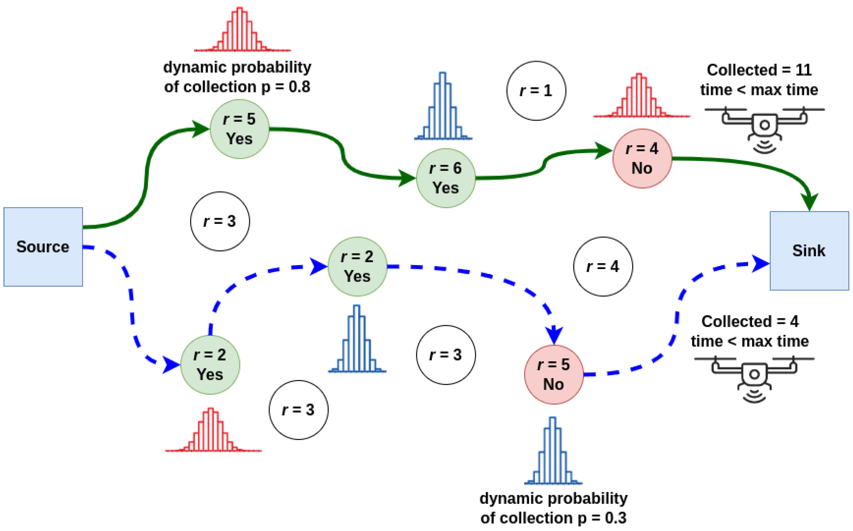
3.1. An Illustrative Example of the DTOP

Figure 1 presents an illustrative example of a simple DTOP. The figure depicts the trajectories of two vehicles, each of them visiting three nodes. From each visited node i in a set N, a vehicle can retrieve (or not) a certain reward $r_i>0$ with a given probability $p_i$. Hence, the actual reward collected by visiting a node $i\in N$ can be $r_i$ with probability $p_i$, or 0 with probability $1-p_i$ (Bernoulli experiment). This probability of success, $p_i$, depends upon the status of some environmental factors (e.g., battery level, weather conditions, etc.) at the time when the node is visited. Nodes with a ‘Yes’ label represent successful reward acquisition, whereas nodes with a ‘No’ label indicate visited nodes where no rewards were obtained. Nodes left unvisited are colored in white. Not all nodes exhibit the same probability values, $p_i$, under varying environmental conditions. To accommodate this variability, we introduce the concept of node types, where each type represents a group of nodes sharing the same probability $p_i$ for a given set of factor values. In other words, nodes within the same type exhibit consistent reward probabilities under similar conditions. Therefore, in our analysis, we consider $k_{max}>1$ distinct types of nodes. This approach results in a DTOP with heterogeneous nodes, meaning that nodes differ in their associated probabilities of reward based on their type.

3.2. A Mathematical Model for the DTOP

This section introduces a mathematical model for the DTOP. The proposed model builds upon the one proposed by Evers et al. [38] for the static TOP. Consider a directed graph $G=(N,A)$, consisting of a set of nodes N, and a set of arcs A. The set $N=\{0,1,2,\dots ,n+1\}$ includes the origin depot (node 0), the destination depot (node $n+1$), and n intermediate nodes offering possible rewards. The set $A=\left\{\right(i,j\left)\right|i,j\in N,i\ne j\}$ represents the connection arcs between nodes. Assume D is the set of heterogeneous vehicles, with each vehicle $d\in D$ starting its route from the origin depot, serving a subset of intermediate nodes, and eventually proceeding to the destination depot. The traveling time for each arc $(i,j)\in A$ is predefined: $t_{ij}=t_{ji}>0$. Each vehicle embarks on a route and can only serve a limited number of nodes due to a travel time constraint for the total route duration, $t_{max}>0$, i.e., each vehicle must reach the endpoint before this time expires. Visiting an intermediate node for the first time yields a reward $r_i>0$ with a probability $p_i$. This probability depends upon several dynamic conditions, including the weather at the node $w_i$, the congestion of the node $c_i$, and the battery level of the vehicle when it reaches the node $b_i$, i.e., $p_i=\varphi (w_i,c_i,b_i)$ for an unknown (black-box) function $\varphi$ emulating reality. The objective is to maximize the total expected rewards collected by all vehicles. Notice that the origin and destination depot do not have any associated reward. For each arc $(i,j)\in A$ and each vehicle $d\in D$, we define a binary variable $x_{ij}^d$, which takes the value 1 if and only if vehicle d traverses the edge $(i,j)$, while otherwise taking the value 0. Additionally, we introduce the variable $y_i^d\ge 0$ to indicate the position of an intermediate node i in the tour made by vehicle d, being $y_0^d=0$ for the origin depot and $y_i^d=0$ if node i is not visited by vehicle d. Then, the mathematical model of the DTOP can be formulated as follows:

$$\begin{array}{cc}\hfill & max\sum _{d\in D}\sum _{(i,j)\in A}{p}_j·r_j·x_{ij}^d\hfill \end{array}$$

(1)

$$\begin{array}{cccc}\mathrm{subject}\mathrm{to}\text{:}\hfill & \sum _{d\in D}\sum _{i\in N}{x}_{ij}^d\le 1\hfill & \hfill & \forall j\in N\hfill \end{array}$$

(2)

$$\begin{array}{cccc}\hfill & y_i^d-y_j^d+1\le (1-x_{ij}^d)\left|N\right|\hfill & \hfill & \forall i,j\in N\forall d\in D\hfill \end{array}$$

(3)

$$\begin{array}{cccc}\hfill & \sum _{(i,j)\in A}{t}_{ij}{x}_{ij}^d\le t_{max}\hfill & \hfill & \forall d\in D\hfill \end{array}$$

(4)

$$\begin{array}{cccc}\hfill & \sum _{i\in N}{x}_{ij}^d=\sum _{h\in N}{x}_{jh}^d\hfill & \hfill & \forall d\in D\forall j\in N\hfill \end{array}$$

(5)

$$\begin{array}{cccc}\hfill & \sum _{j\in N}{x}_{0j}^d=1\hfill & \hfill & \forall d\in D\hfill \end{array}$$

(6)

$$\begin{array}{cccc}\hfill & \sum _{i\in N}{x}_{i(n+1)}^d=1\hfill & \hfill & \forall d\in D\hfill \end{array}$$

(7)

$$\begin{array}{cccc}\hfill & y_j^d\ge 0\hfill & \hfill & \forall j\in N\forall d\in D\hfill \end{array}$$

(8)

$$\begin{array}{cccc}\hfill & x_{ij}^d\in \{0,1\}\hfill & \hfill & \forall (i,j)\in A\forall d\in D\hfill \end{array}$$

(9)

Unlike the traditional TOP, which aims to maximize the total collected rewards, Equation (1) in our model incorporates a probabilistic factor, $p_j$, that accounts for the dynamic nature of real-world scenarios. This factor reflects the probability of obtaining the reward $r_j$ at node j based on the current status of the environmental conditions. Constraints (2) ensure that each node in the network is serviced at most once, avoiding repetitive visits by any vehicle. To prevent the formation of subtours within the routes, Constraints (3) are imposed. The travel time constraint for each vehicle, given in Constraints (4), ensures that the total travel time for any route does not exceed a predefined maximum. Flow balance across the network is maintained by Constraints (5), which stipulate that the number of times a vehicle enters a node must equal the number of times it exits. Each vehicle’s route is required to start at the origin depot and end at the destination depot, as defined in Constraints (6) and (7). Lastly, the non-negative and binary nature of the variables $y_j^d$ and $x_{ij}^d$, respectively, are established in Constraints (8) and (9).

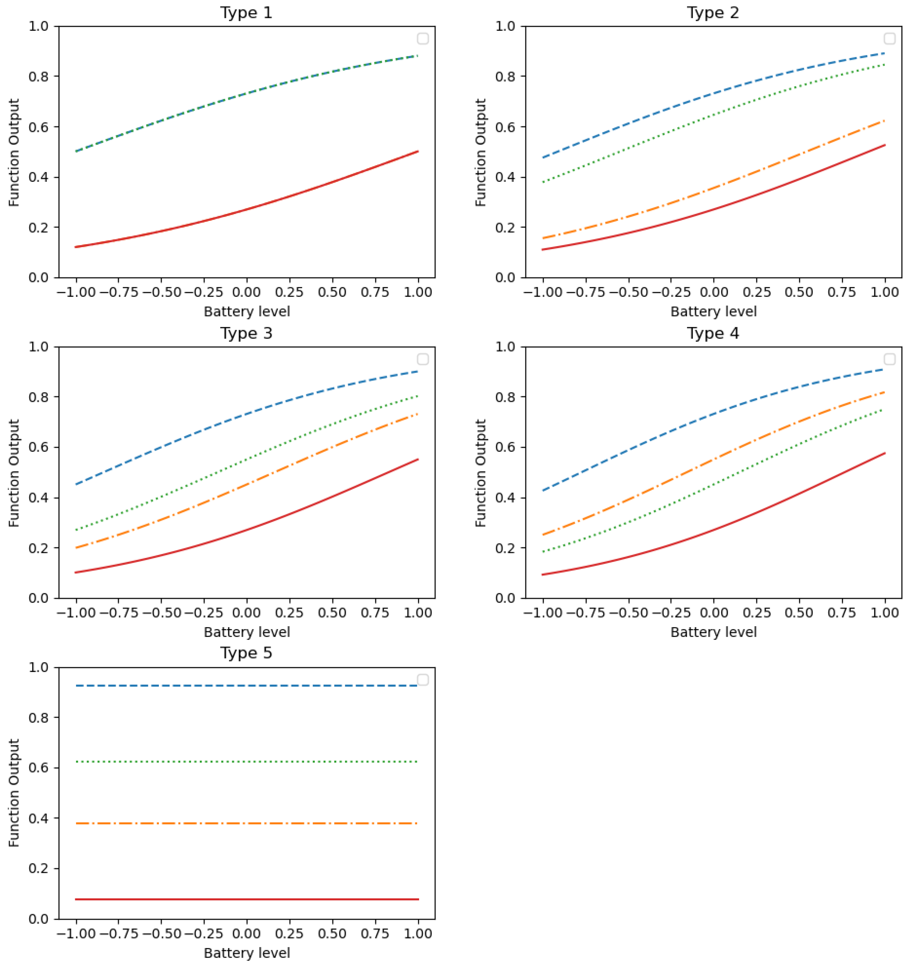
4. Modeling Probabilities of Reward for Different Types of Nodes

To emulate real-life environmental conditions, a ‘black-box’ function is implemented. The term black-box refers to the fact that the function internal behavior is not accessible to the solving algorithm, which will only be able to provide inputs to the black-box function and obtain outputs, thus emulating a real-life environment with unknown internal behavior. In our numerical experiments, this black-box has been implemented using a logistic regression model [39]. In particular, our black-box model considers factors such as weather conditions, congestion levels, and the remaining battery percentage of an electric vehicle, as follows:

$$\varphi (w,c,b)=\frac{1}{1+e^{{\beta }_0+{\beta }_1·w+{\beta }_2·c+{\beta }_3·b}}$$

(10)

where:

• Parameter $w\in \{0,1\}$ implies the meteorological conditions: a value 0 denotes good meteorological conditions, whereas a value 1 expresses bad ones.
• Parameter $c\in \{0,1\}$ represents the congestion level in the urban network: a value 1 denotes severe congestion on the node, whereas a value 0 expresses the lack of it.
• Parameter $b\in [0,1]$ indicates the remaining battery percentage of an electric vehicle: a value 1 denotes that the battery is full of energy, whereas a value 0 express that the battery is empty.

The black-box function utilizes a set of $\beta$ coefficients, namely ${\beta }_0$, ${\beta }_1$, ${\beta }_2$, and ${\beta }_3$, to model the effect of these variables on the routing process:

• Coefficient ${\beta }_0$ acts as a baseline intercept term, representing the default scenario when all variables are at their baseline levels.
• Coefficient ${\beta }_1$ modulates the influence of meteorological conditions (w).
• Coefficient ${\beta }_2$ reflects the impact of congestion (c) at the specific node being visited.
• Coefficient ${\beta }_3$ adjusts the outcome based on the remaining battery percentage (b).

In the proposed DTOP, the environmental conditions can change while the vehicles are in motion. For example, a node that starts off without congestion when the route begins may become congested as the vehicles progress, making it less attractive to visit. Moreover, not all nodes react the same way to these changes in environmental conditions, particularly in terms of their associated probabilities $p_i$. To account for this variability among nodes, we categorize them into $k_{max}$ different types based on their likelihood of providing rewards under different environmental circumstances. To ensure consistency and reproducibility in our experiments, we assign each node $i\in \{1,2,\dots ,n\}$ a specific type using the following expression:

$$\mathrm{type}\mathrm{of}\mathrm{node}i=imod{k}_{max}$$

(11)

In Equation (11), the operation $imod{k}_{max}$ calculates the remainder when i is divided by $k_{max}$. This approach enables us to classify nodes into $k_{max}$ distinct categories, each representing a unique aspect of the black-box function. Utilizing modular division ensures an even distribution of these node types across the network and adds complexity to the reward system.

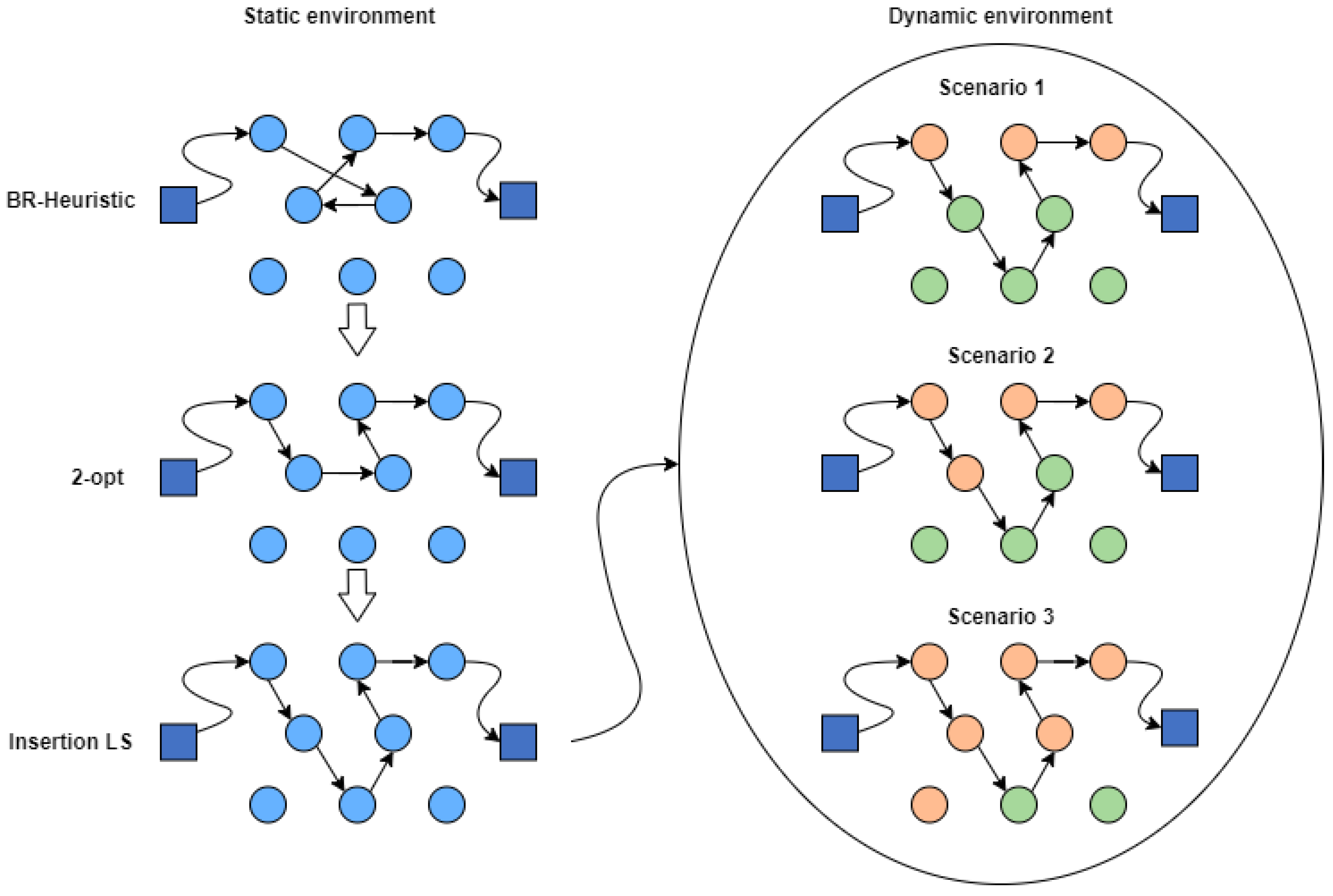
5. Solution Approaches for the Heterogeneous DTOP

In order to solve the heterogeneous DTOP, we propose a learnheuristic algorithm that capitalizes on the strengths of Thomson sampling [40] for dealing with the unkonwn values of the probabilities $p_i$. In particular, Thomson sampling is employed to build a ‘white-box’ reinforcement learning mechanism that predicts the performance of the black-box function, which is unknown for the algorithm. To assess the effectiveness of the learnheuristic algorithm, we first describe a traditional constructive algorithm that does not consider either dynamism or real-time conditions. Hence, this can be denoted as a static algorithm. Next, we propose a dynamic algorithm where nodes are selected in real time based on the information provided by the Thomson sampling.

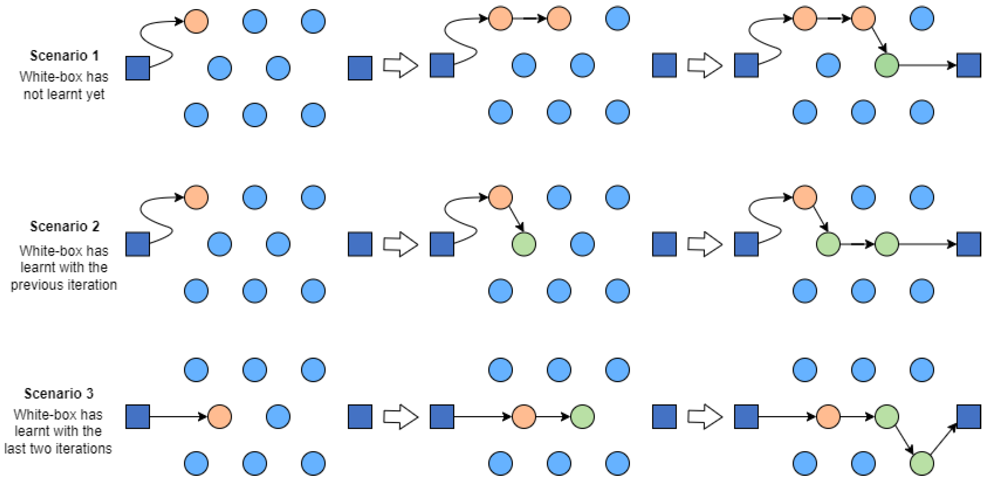
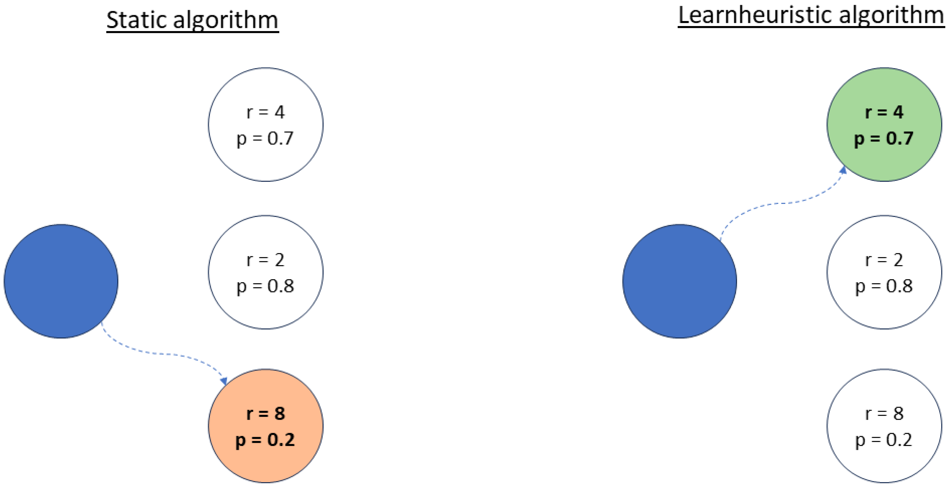
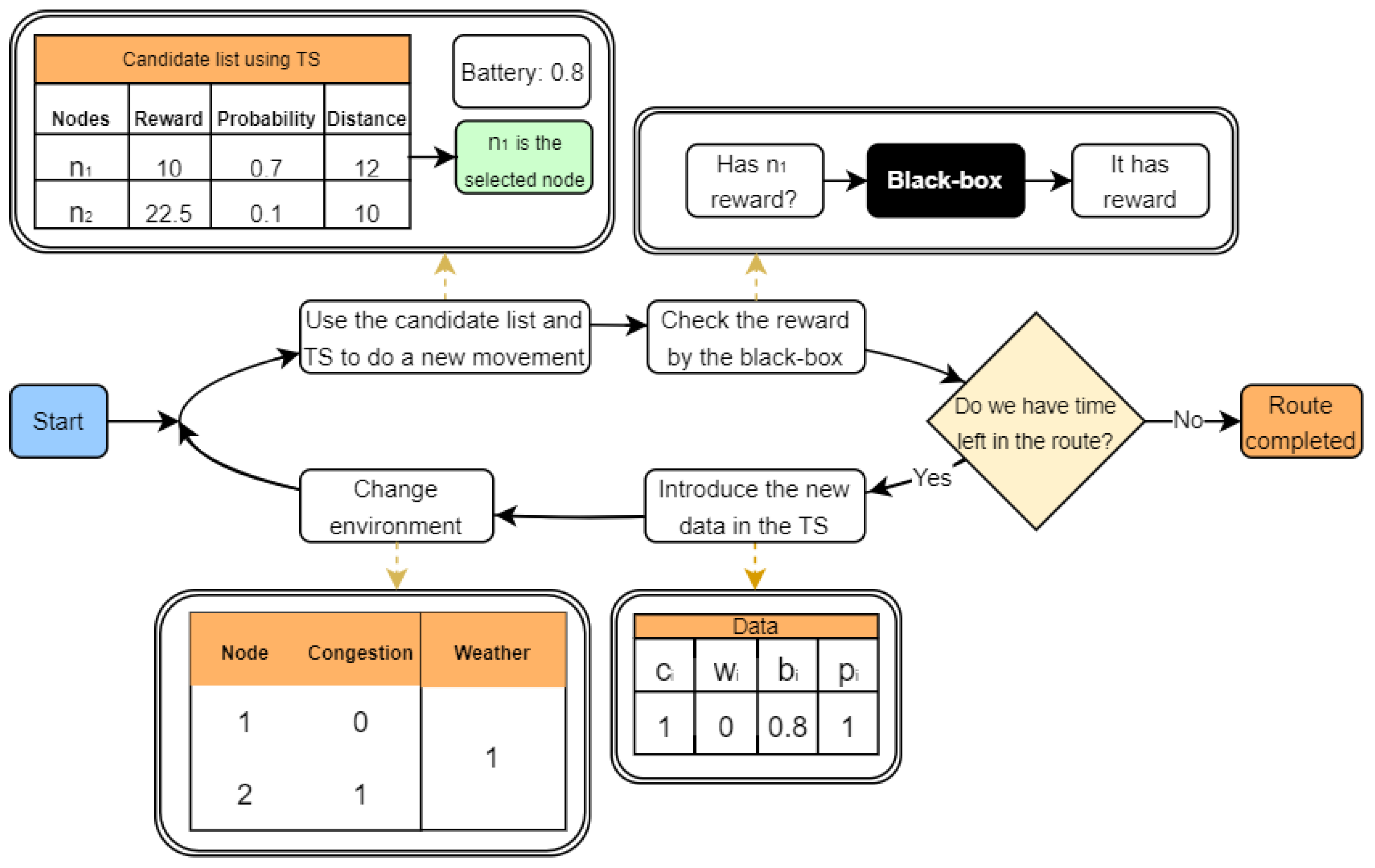
5.1. Online Contextual Thompson Sampling

Thompson sampling [41] is a heuristic strategy used in decision-making scenarios like the multi-armed bandit problem (MABP) [42]. This method is used for choosing actions according to their expected rewards, which are continuously updated using Beta probability distributions based on previous successes and failures [43]. In the context of the heterogeneous DTOP discussed in this article, each node type is analogous to an arm in a contextual MABP setup. To estimate the success probability of each node, we apply a regularized Bayesian logistic regression as described in Chapelle and Li [44]. Thus, for each node type $k\in \{1,2,\dots ,k_{max}\}$, the probability ${\pi }_k\left(x\right)$ under the vector of factor values x is estimated as

$${\pi }_k\left(x\right)=\frac{1}{1+exp(-f(x\left)\right)}$$

(12)

where

$$f\left(x\right)={\beta }_0+{\beta }_1·x+ϵ$$

(13)

and the weights ${\beta }_i$ are distributed as independent Gaussian probability distributions, as follows:

$${\beta }_i=\mathcal{N}(m_i,\alpha ·q_i^{-1})$$

(14)

This algorithm is particularly effective in online settings and features an adjustable learning rate $\alpha >0$. For $\alpha >1$, the model incentivizes exploration, and for $\alpha <1$, the model is more exploitative. The process for fitting this model is outlined in Chapelle and Li [44]. Examples of the latest use of Thompson Sampling can be found in [45,46].

5.2. A Static Constructive Heuristic

Algorithm 1 shows the main procedure of the static constructive heuristic without considering the predictions provided by the white-box to deal with the dynamic conditions of the problem. The algorithm employs a parameter $\gamma$, which allow us to define a geometric probability distribution associated with a BR approach [47], performed in get_candidate function in line 6, as well as a parameter $\delta$, used to calculate the efficiency list [10]. To determine the $\delta$ parameter, we execute the constructive heuristic 10 times, adjusting $\delta$ within the range of 0 to 1 in increments of 0.1 for each run. The $\delta$ value that produces the best solution is then utilized for the entire execution. In line 1, the algorithm is initialized, setting empty to $Routes$. Then, whereas not all routes are completed, each one is constructed (line 2). Line 3 initializes a route to complete. The function evaluate_efficiency (line 5) evaluates each node and is described in Equation (15). BR appproach is performed in line 6 to obtain a candidate. Then, that candidate is added to the route R in line 7. Function exceed_max_distance (line 8) determines when a route R under construction if finished, and then can mark the route R as complete and can be aggregated to the solution (lines 9, 10, 11). Update the objective function with the built route (line 14).

Algorithm 1 Constructive Static Solution ($\gamma$, $\delta$)

1: $Routes\leftarrow \varnothing$ 2: while all_routes_complete$\left(Routes\right)$ do 3:     $R\leftarrow \varnothing$ 4:     while is_incomplete$\left(R\right)$ do 5:         $candidates\leftarrow$ evaluate_efficiency$(N,\delta )$ 6:         $i\leftarrow$ get_candidate$(candidates,\gamma )$ 7:         $R\leftarrow R\cup \left\{i\right\}$ 8:         if exceed_max_distance$(i,R)$ then 9:            Mark R as complete. 10:            $R\leftarrow R\setminus \left\{i\right\}$ 11:            $Routes\leftarrow Routes\cup R$ 12:            $break$ 13:         end if 14:         Update_OF$\left(R\right)$ 15:     end while 16: end while 17: return Routes

The constructive static solution approach begins by initializing an empty set named $Routes$. The algorithm proceeds iteratively while the number of routes is less than the number of vehicles available. For every vehicle, the algorithm first calculates a set of candidate nodes that could potentially be added to the current route. This set of candidates is determined by the evaluate_efficiency function according to the following expression:

$$eval\left(i\right)=\delta ·\left(1-\frac{distance(last\_node(v),i)}{max\_distance(\mathit{N}\setminus \mathit{R})}\right)+(1-\delta )·\frac{r_i}{max\_reward(\mathit{N}\setminus \mathit{R})}$$

(15)

where last_node$\left(v\right)$ corresponds to the last node visited in the route and $r_i$ corresponds with the reward of node i. Both values are normalized by the $max\_distance$ and $max\_reward$ of the nodes not in the solution set (R). Once the candidates are determined, the algorithm selects the most suitable candidate node i using the $get\_candidate$ function. This function can be a greedy one where you select the best node or, like in our case, a BR one that allows us to select a node randomly but assigns higher probabilities to the most ‘promising’ ones. It then adds the node to the vehicle’s route and updates the route details and the objective function ($OF$) accordingly. However, if adding the node exceeds the maximum distance, the current route of vehicle R is marked as complete and is added to the set Routes. This process is repeated until all routes are completed. The algorithm concludes by returning the set Routes, which contains the constructed routes for all vehicles. Once a preliminary solution is obtained, the local search algorithm is employed to enhance it.

A 2-opt local search is employed to derive a solution aimed at reducing the total travel time to reduce travel time and allow for the inclusion of new nodes in the solution. Specifically, whenever a proposed arc swap yields a better solution than the current configuration. Subsequently, we attempt to incorporate additional nodes using the methodology outlined in Algorithm 1, continuing this process until the maximum allowable distance is reached. Figure 2 shows the process flow of the static algorithm. The initial step involves constructing a solution via the BR, as outlined in Algorithm 1. Following the construction of an initial solution, it is refined through a 2-opt optimization. Subsequently, an additional local search (LS) is conducted to ascertain any further enhancements, culminating in the iteration’s final solution. Lastly, this solution is tested within a dynamic environment to evaluate the performance of the static solution under changing conditions.

The static constructive algorithm exhibits a complexity that can be analyzed by the constructive node selection process, which uses $O(n^2·log\left(n\right))$. This is attributed to the operations involved in identifying the closest node to a given point and subsequently sorting these values, where n represents the number of nodes. Constraint checks, such as the maximum distance, are performed at each step of route construction, maintaining the $O(m·n)$ complexity, where m represents the number of vehicles. The application of a 2-opt local search post-construction, typically $O\left(n^2\right)$ for route optimization, further influences the overall complexity. Thus, the algorithm’s total complexity can be approximated as $O(m·n^2·log\left(n\right)+m·n+n^2)$, acknowledging that the heuristic and probabilistic elements introduce variability that may affect the actual performance in practice. It is essential to emphasize that the static algorithm, generates a single static solution before its exposure to a dynamic environment. This solution, once obtained, is subjected to simulations across various dynamic scenarios. However, the complexity and time required to derive this static solution remain independent of the number of dynamic scenarios in which it is subsequently simulated.

5.3. A Learnheuristic Constructive Heuristic

The dynamism inherent in the problem presents a new challenge: the algorithm should adapt its performance using contextual data. This learning mechanism is detailed in Section 5.1. The algorithm receives inputs from a predictive white-box model, providing feedback on the likelihood of encountering rewards at different nodes. The primary distinction between this new Algorithms 2 and Algorithm 1 lies in the way the node efficiency is computed (line 6), described in Equation (16).

Algorithm 2 Constructive Dynamic Solution ($\gamma$, $\delta$)

1: $Routes\leftarrow \varnothing$ 2: $weather,congestion=$ new_environment() 3: while all_routes_complete$\left(Routes\right)$ do 4:     $R\leftarrow \varnothing$ 5:     while is_incomplete$\left(R\right)$ do 6:         candidates ← evaluate_efficiency_with_wb$(N,\delta )$ 7:         $i\leftarrow$ get_candidate$(candidates,\gamma )$ 8:         $R\leftarrow R\cup \left\{i\right\}$ 9:         if exceed_max_distance$(i,R)$ then 10:            Mark R as complete 11:            $R\leftarrow R\setminus \left\{i\right\}$ 12:            $Route\leftarrow Route\cup R$ 13:            $break$ 14:         end if 15:         Update_OF$\left(R\right)$ 16:         weather, congestion = new_environment() 17:     end while 18: end while 19: return $Routes$

In the dynamic context, we introduce the $\pi \in [0,1]$ parameter, derived from the white-box model based on factors like weather, node congestion, and battery level. The node evaluation formula is as follows:

$$eval\left(i\right)=\delta ·\left(1-\frac{distance(last\_node(v),i)}{max\_distance(\mathit{N}\setminus \mathit{R})}\right)+(1-\delta )·{\pi }_i·\frac{r_i}{max\_reward(\mathit{N}\setminus \mathit{R})}$$

(16)

Therefore, whereas the static algorithm operates by generating multiple solutions initially and then evaluating these solutions within a dynamic context, the dynamic (learnheuristic) algorithm is characterized by its ability to operate in a constantly evolving environment. It does not generate multiple solutions. Instead, it adapts and recalculates solutions as the environment changes with each node selection. The algorithm is required to make real-time decisions without the ability to plan multiple steps. One critical consideration in the dynamic algorithm is the avoidance of local search methods. This is due to the potential reduction in rewards and increased complexity by the real-time changes in the environment. Every inclusion of a node into an emerging solution alters the environment. Figure 3 shows the flow of the learnheuristic algorithm. Throughout its execution, the algorithm records data pertaining to each visited node including congestion levels, weather conditions, and battery status as well as the node’s state regarding reward availability. This information is systematically compiled by vehicles through sensors and communication technologies embedded in them, sent to the central system, and utilized to calibrate the Thompson sampling model, improving its predictive accuracy for future iterations and generating a data traffic scheme specific to the IoT framework.

In Figure 4, the principal distinctions in the decision-making process for choosing a node are illustrated. The static algorithm, which does not utilize any predictive models, selects nodes based on distance and reward, regardless of the associated probability of actually receiving that reward. This approach may lead to choices where the likelihood of obtaining a reward is quite low. In contrast, the learnheuristic algorithm incorporates predictive analytics into its decision-making process. It utilizes information from a Thompson sampling predictor to make more informed choices. This method allows for a more strategic selection of nodes, taking into account not only the reward amount but also the probability of successfully obtaining that reward based on the predicted probability values.

The complexity of the dynamic algorithm reflects its adaptability to a changing environment. The node selection process, similar to the static algorithm, maintains a complexity of $O(n^2·log\left(n\right))$, considering the sorting and evaluation steps. However, the unique characteristic of this dynamic algorithm lies in its real-time adaptation to environmental changes, necessitating frequent recalculations with each node selection. In fitting a Thompson sampling model, the complexity primarily arises from two operations: updating the probability distributions of rewards and sampling from these distributions. Assuming constant-time operations for updates and sampling, the complexity for each type of node, in a scenario with $k_{max}$ node types, can be approximated as $O\left(n\right)$ per iteration. Additionally, the avoidance of local search methods, while reducing complexity in one aspect, is offset by the continuous recalibration based on the evolving environment and the systematic recording and utilization of data for the Thompson sampling model. Consequently, the baseline complexity of the dynamic algorithm can be approximated at $O(n^2·log\left(n\right)+n)$ for the node selection process and prediction of Thompson sampling. This complexity must be multiplied by the number of dynamic scenarios that have to be run.

6. Numerical Experiments

This section outlines the computational experiments we conducted to evaluate the efficacy and performance of the previously discussed algorithms. All algorithms were implemented using Python version $3.11$ and executed on a Google cloud platform computing instance [48] equipped with an AMD EPYC 7B12 CPU @ $2.25$ GHz, 4 GB of RAM, and a Debian 11 operating system. For experimental purposes, we utilized the benchmark set proposed by [3], as it is widely employed in the literature to assess the performance of algorithms designed to solve the classical version of the TOP. This benchmark set is divided into seven different subsets, containing a total of 320 instances. Within each subset, the node locations and rewards remain constant across all instances. However, the number of vehicles, m, as well as the time threshold, $T_{max}$, can vary. The naming convention for each instance follows the format pa.b.c, where (i) a represents the identifier of the subset; (ii) b is the number of vehicles, which varies between 2 and 4; and (iii) c denotes an alphabetical order for each instance. We performed 100 iterations for each instance except for those belonging to subset $p7$, for which we conducted 1000 iterations due to their larger size. Each run has its own parameters for congestion and weather, defined by the seed. For each node added to the solution, the parameters change by incrementing the seed by 1. In the experiments, three distinct seeds were used to create the environments of the instances. Once a simulation has run, the seed will change by adding 10,000 to generate a different scenario. Figure 5 illustrates the random sampling process in the problem. We selected a node to visit based on Thompson Sampling (TS), which provides the probability of a node having a reward. From the list of candidates, we chose one of these nodes. The black box indicates whether the selected node has a reward associated with it. Using this information, we updated the TS data, refining the model to generate more accurate results. We then adjusted the nodes’ environment, accounting for potential changes in congestion and weather conditions. We continued this process until the drone ran out of battery, thereby completing the solution.

We compared the effectiveness of the proposed dynamic approach against a static one, where the latter operates without integrating the learned insights from the white-box model. For the static method, we chose the PJHeuristic [10], a powerful and widely validated heuristic for solving the deterministic TOP. Specifically, the deterministic method assumes that $\pi \left(n_i\right)=1,\forall i\in V$.

For conducting the numerical experiments, it is necessary to establish the black-box parameters, which determine the varying probabilities of earning rewards at each node, depending on environmental conditions. In the design of the experiment carried out, the betas have been selected in such a way that the probability curves were sufficiently different depending on the established magnitude of difference (Low, Medium, High) and had coherent probabilities. In our analysis, the variables have been standardized to a range of $-1$ to 1 in order to ensure consistency and comparability. In order to create node types that are stable in terms of probability when all conditions are neutral, ${\beta }_0$ is set to 0 for all scenarios. For instance, ${\beta }_1$ is assigned a negative sign, indicating that better weather conditions improve the probability of receiving a reward. Similarly, ${\beta }_2$, which is linked to traffic congestion, also follows this standardized scale. On the other hand, ${\beta }_3$ carries a positive sign, reflecting an increase in the probability of reward when the battery is fully charged (represented by 1) and a decrease when the battery is low (represented by $-1$). This standardization of values facilitates a clearer understanding and interpretation of their impact on reward probabilities. In our experiments, we have set $k_{max}=5$, i.e., a total of five types of nodes have been considered, each with distinct parameters and behaviors. For example, the probability associated with type node 5 is independent of the battery level. We have also established three sets of dynamism, each representing a different level of variability. With higher levels of dynamism, environmental conditions play a more significant role in determining the probability of receiving a reward.

Table 1. Black-box’s parameters employed with Equation (10).

Node Type	Low			Medium			High
	${\mathit{\beta }}_{\mathbf{1}}$	${\mathit{\beta }}_{\mathbf{2}}$	${\mathit{\beta }}_{\mathbf{3}}$	${\mathit{\beta }}_{\mathbf{1}}$	${\mathit{\beta }}_{\mathbf{2}}$	${\mathit{\beta }}_{\mathbf{3}}$	${\mathit{\beta }}_{\mathbf{1}}$	${\mathit{\beta }}_{\mathbf{2}}$	${\mathit{\beta }}_{\mathbf{3}}$
N1	0	−1	1	0	−1.2	1.2	0	−2	1
N2	−0.2	−0.8	1.1	−0.4	1	1.4	−0.6	−1.5	2
N3	−0.4	−0.6	1.2	−0.6	−0.8	1.6	−1.2	−1	3
N4	−0.6	−0.4	1.3	−0.8	−0.6	1.8	−1.8	−0.8	4
N5	−1	−1.5	0	−1.5	−2	0	−2	−3	0

provides detailed information on the probability of each node providing the possible reward. This probability is calculated based on various scenarios that combine factors such as weather, congestion, and battery level. Notice that the battery level significantly influences this probability for most types of nodes. Figure 6 depicts a graphical representation of the five different types of nodes in the low-level scenario. The color coding represents different environmental conditions to generate heterogeneous nodes: blue lines indicate good weather and no congestion, green lines represent bad weather without congestion, yellow lines indicate good weather with congestion, and red lines denote bad weather coupled with severe congestion. This color scheme provides a clear visual representation of how different environmental factors affect the probability of receiving rewards at each node. Node types can be more affected by some environmental conditions than others.

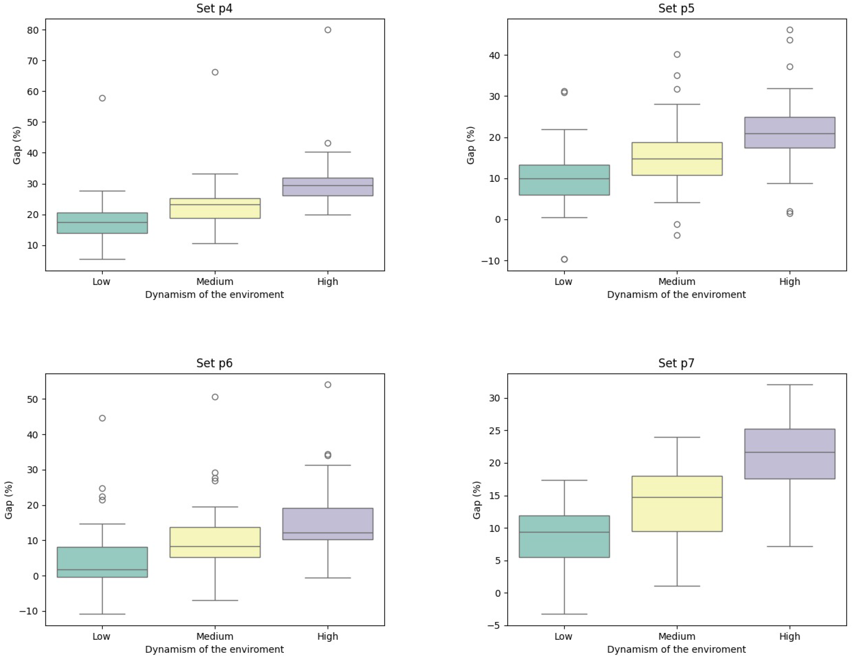
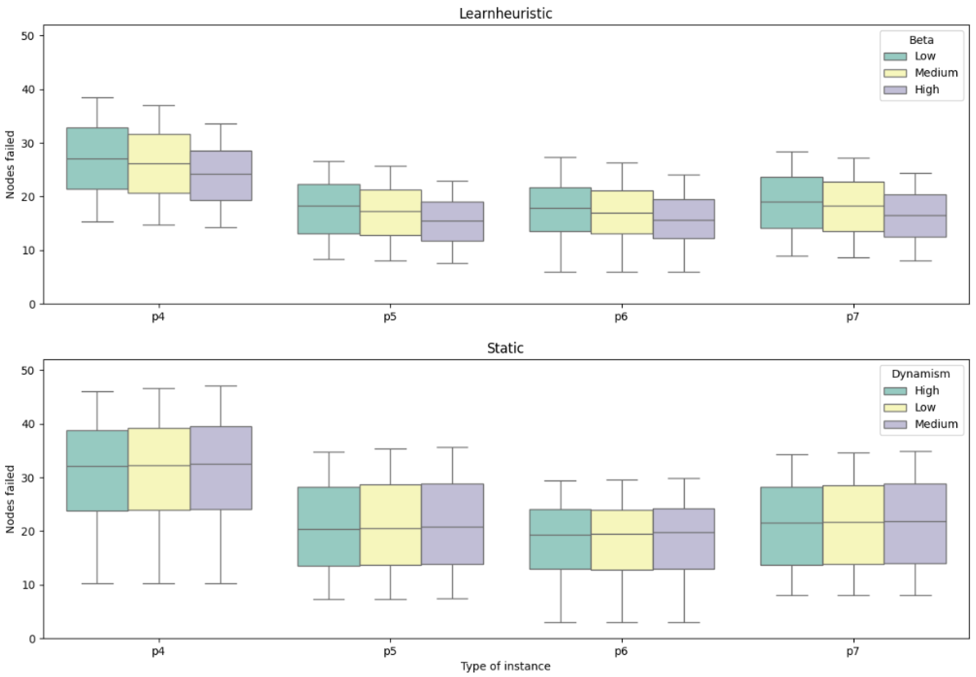
7. Analysis of Results

As observed in

Table 2. Comparative results between learnheuristic and static algorithms.

Instance	Static									Learnheuristic									Gap (%)
	Low (1)			Medium (2)			High (3)			Low (4)			Medium (5)			High (6)
	Time	OF	Dyn. OF	Time	OF	Dyn. OF	Time	OF	Dyn. OF	Time	OF	Dyn. OF	Time	OF	Dyn. OF	Time	OF	Dyn. OF	(1)–(4)	(2)–(5)	(3)–(6)
p4.2	12.07	901.90	431.54	12.02	876.17	428.36	12.03	901.90	437.75	23.06	804.40	492.11	23.00	800.48	512.88	22.77	796.39	551.54	14.04%	19.73%	25.99%
p4.3	10.71	804.40	384.37	10.64	804.40	381.14	10.66	804.40	388.59	19.71	728.19	449.91	19.68	726.84	464.95	19.57	724.11	503.12	17.05%	21.99%	29.47%
p4.4	9.30	677.13	323.75	9.31	652.40	321.59	9.24	652.40	329.19	16.15	632.55	389.08	16.12	632.55	404.64	16.07	630.45	436.25	20.18%	25.83%	32.52%
p5.2	4.98	995.00	460.21	4.99	995.00	456.15	4.98	995.00	470.05	9.59	808.99	491.18	9.58	805.59	509.95	9.59	804.18	554.34	6.73%	11.79%	17.93%
p5.3	4.53	843.56	391.34	4.51	843.56	387.32	4.49	843.56	398.28	8.50	703.94	430.44	8.48	700.71	445.13	8.47	698.28	480.76	9.99%	14.93%	20.71%
p5.4	4.17	718.94	331.94	4.16	718.94	328.33	4.17	718.94	337.54	7.49	607.85	372.75	7.49	607.20	386.45	7.49	602.68	416.14	12.29%	17.70%	23.28%
p6.2	4.84	868.60	411.58	4.83	868.60	406.55	4.84	868.60	411.90	9.54	703.31	424.62	9.53	704.34	441.83	9.53	702.32	476.01	3.17%	8.68%	15.56%
p6.3	4.74	766.58	363.46	4.71	766.58	358.49	4.69	766.58	364.34	9.08	670.13	391.32	9.06	667.54	403.94	9.06	662.22	426.72	7.67%	12.68%	17.12%
p6.4	4.37	664.00	315.66	4.44	664.00	310.76	4.42	664.00	317.22	8.51	633.14	354.50	8.52	631.78	365.79	8.45	622.72	384.12	12.31%	17.71%	21.09%
p7.2	82.17	700.16	332.47	84.15	700.16	329.20	84.10	700.16	335.54	157.27	581.28	360.32	157.12	579.53	373.86	155.19	570.09	401.66	8.37%	13.57%	19.70%
p7.3	77.82	650.45	307.38	77.33	650.45	304.01	77.41	650.45	310.06	136.70	544.72	335.94	136.43	543.56	349.74	135.88	316.64	469.32	9.29%	15.04%	51.37%
p7.4	67.27	547.23	259.14	67.15	547.21	256.89	67.05	547.21	262.05	108.88	472.65	293.58	109.25	472.42	306.31	107.99	467.08	332.55	13.29%	19.24%	26.90%
Average	23.92	761.49	359.40	24.02	757.29	355.73	24.01	759.43	363.54	42.87	657.60	398.81	42.86	656.04	413.79	42.50	633.10	452.71	11.20%	16.57%	25.14%
Instance	Static						Learnheuristic						Gap (%)
	Low (1)		Medium (2)		High (3)		Low (4)		Medium (5)		High (6)		(1)–(4)	(2)–(5)	(3)–(6)
	Nodes	Fails	Nodes	Fails	Nodes	Fails	Nodes	Fails	Nodes	Fails	Nodes	Fails
p4.2	60.62	33.23	60.62	33.52	60.62	32.93	59.62	27.59	59.19	26.36	58.71	23.93	−16.97%	−21.37%	−27.33%
p4.3	56.77	31.65	56.77	31.94	56.77	31.47	56.68	27.19	56.49	26.36	56.14	24.11	−14.10%	−17.48%	−23.39%
p4.4	51.33	29.31	51.33	29.52	51.33	29.00	52.76	26.77	52.71	25.94	52.46	24.07	−8.66%	−12.12%	−16.99%
p5.2	38.50	21.61	38.50	21.78	38.50	21.29	36.60	17.05	36.51	16.23	36.47	14.50	−21.10%	−25.46%	−31.93%
p5.3	36.48	20.91	36.48	21.07	36.48	20.67	36.07	17.70	35.99	16.96	35.92	15.41	−15.34%	−19.49%	−25.45%
p5.4	34.65	20.39	34.65	20.53	34.65	20.17	35.57	18.52	35.57	17.87	35.47	16.38	−9.20%	−12.98%	−18.79%
p6.2	38.50	21.18	38.50	21.40	38.50	21.20	37.89	17.63	37.85	16.88	37.78	15.25	−16.75%	−21.14%	−28.05%
p6.3	39.17	22.00	39.17	22.26	39.17	22.03	40.49	20.63	40.38	19.92	40.25	18.67	−6.24%	−10.53%	−15.23%
p6.4	38.13	21.81	38.13	22.06	38.13	21.80	42.89	23.51	42.87	22.82	42.59	21.52	7.83%	3.43%	−1.28%
p7.2	41.50	22.95	41.50	23.13	41.50	22.72	39.77	18.43	39.60	17.67	39.12	15.78	−19.70%	−23.60%	−30.55%
p7.3	38.54	21.81	38.54	21.97	38.54	21.61	38.64	19.19	38.52	18.45	38.23	16.65	−12.03%	−16.03%	−22.93%
p7.4	35.63	20.70	35.63	20.84	35.63	20.49	37.65	19.87	37.60	19.21	37.19	17.52	−3.99%	−7.83%	−14.46%
Average	42.49	23.96	42.49	24.17	42.49	23.78	42.89	21.17	42.77	20.39	42.53	18.65	−11.35%	−15.38%	−21.36%

, on average, the solutions obtained from the dynamic approach outperform the deterministic solutions when they are evaluated in dynamic scenarios for all the tested cases. Specifically, in dynamic environments, the performance gap between these methodologies ranges from 11.20% in low-dynamism scenarios to 25.14% in highly dynamic scenarios, whereas the static algorithm shows enhanced efficiency in static scenarios (column OF), the learnheuristic algorithm outperforms it in dynamic contexts. It is noteworthy that the computational time of the static method only accounts for the generation of a single solution, whereas the dynamic approach iteratively produces multiple solutions, specifically, 100 distinct iterations for instances other than $p_7$ and 1000 iterations for $p_7$ instances. Consequently, in data-rich environments, the dynamic algorithm can yield superior outcomes in a comparably shorter time frame. All disaggregated data by instance, including detailed performance metrics and analysis results, are publicly available at: https://github.com/juanfran143/Dynamic_TOP (accessed on 2 May 2024).

Figure 7 and Figure 8 depict the comparative results of our learnheuristic approach and the deterministic method employed. Specifically, Figure 7 illustrates the gaps between the static and learnheuristic approaches for the four different sets of tested instances and levels of environmental dynamism, where the discontinuous line represents the base deterministic solution obtained using the PJHeuristic and simulated in the dynamic scenario. Each subplot corresponds to a specific instance and not only clarifies the trend of an increasing performance gap with escalating levels of environmental dynamism—from low to medium to high— but also highlights that the vast majority of these gaps are positive. This indicates that the learnheuristic algorithm has a better capacity to adapt and generally yields superior results in dynamic settings. On the other hand, Figure 8 depicts the distribution of fail nodes, highlighting the algorithm’s robustness in maintaining node integrity across instances $p4$ to $p7$. Thus, the learnheuristic approach demonstrates a greater capacity to avoid nodes with a higher likelihood of failure in more dynamic environments, and whereas the probability of obtaining a reward in low-dynamic settings is approximately 0.6, this probability can increase to 0.9 in highly dynamic environments. The analysis of node failures and performance discrepancies across various instance types enhances our understanding of algorithmic efficacy in dynamic scenarios. Notice that near-optimal solutions obtained using a deterministic approach can be sub-optimal or even infeasible (with a total collected reward of 0) in dynamic scenarios. Thus, the proposed learnheuristic is able to provide solutions with superior performance in such scenarios. Although we have used PJHeuristic as the deterministic approach because it is widely used in the literature to solve the TOP, its behavior in dynamic scenarios can be extrapolated to any other deterministic heuristic due to the lack of mechanisms to consider dynamic components during their optimization procedures.

8. Conclusions and Future Work

This study has analyzed the Dynamic Team Orienteering Problem, focusing on the comparative effectiveness of learnheuristic approaches against static methods under varying degrees of dynamism. Our findings revealed that the learnheuristic approach shows a significant enhancement in performance, which grows as the level of dynamism increases. In environments characterized by low dynamism, both the learnheuristic and static algorithms exhibited similar levels of performance, with the learnheuristic algorithm showing a modest improvement, reflected in a gap of $11.20\%$. However, as the dynamism shifted to a medium level, the learnheuristic algorithm began to outshine its static version, delivering more significantly improved solutions with a gap of $16.57\%$.

A critical consideration, however, is the accessibility of real-time data. Despite the learnheuristic approach having excellent results, it is crucial to acknowledge that not all companies have access to real-time data, and the additional costs associated with acquiring such data may not be justifiable for every business. In scenarios where companies must assume a static environment due to the lack of real-time information, the deterministic algorithm provides a better solution, as it is specifically customized for these circumstances. This highlights a limitation of the learnheuristic approach in contexts where dynamic data are unavailable to obtain.

The advantage of the learnheuristic approach became particularly evident in high dynamism scenarios, where its capacity to adeptly adapt to rapid changes and complex decision-making processes in real-time urban settings was unparalleled, showing an improvement of $25.14\%$ compared to the static algorithm. Despite the longer computational times associated with the learnheuristic method, the gains in accuracy and adaptability in dynamically challenging environments justified the trade-off. The algorithm’s ability to process and respond to live data streams significantly contributed to its superior performance in managing the intricacies of urban logistics and electric vehicle integration. In the problem described, failing at a node means not obtaining the reward. However, there are other possible variants of the problem where either a minimum level of reliability is required, or failing to obtain the reward could lead to a negative impact on the objective function. This learnheuristic approach has even greater potential in these scenarios.

Future research will aim at retaining the learnheuristic robustness and precision. Additionally, improving the complexity and operational efficiency of the algorithm is a key area for enhancement, as the current algorithm’s runtime is nearly twice that of static algorithms. Further exploration into integrating more detailed real-time data and extending the application of these algorithms to larger and more intricate urban settings are also topics to be explored in more detail.

References

1. Archetti, C.; Speranza, M.G.; Vigo, D. Chapter 10: Vehicle routing problems with profits. In Vehicle Routing: Problems, Methods, and Applications, 2nd ed.; SIAM: Philadelphia, PA, USA, 2014; pp. 273–297. [Google Scholar]
2. Butt, S.E.; Cavalier, T.M. A heuristic for the multiple tour maximum collection problem. Comput. Oper. Res. 1994, 21, 101–111. [Google Scholar] [CrossRef]
3. Chao, I.M.; Golden, B.L.; Wasil, E.A. The team orienteering problem. Eur. J. Oper. Res. 1996, 88, 464–474. [Google Scholar] [CrossRef]
4. Vansteenwegen, P.; Souffriau, W.; Van Oudheusden, D. The orienteering problem: A survey. Eur. J. Oper. Res. 2011, 209, 1–10. [Google Scholar] [CrossRef]
5. Gunawan, A.; Lau, H.C.; Vansteenwegen, P. Orienteering problem: A survey of recent variants, solution approaches and applications. Eur. J. Oper. Res. 2016, 255, 315–332. [Google Scholar] [CrossRef]
6. Vansteenwegen, P.; Souffriau, W.; Berghe, G.V.; Van Oudheusden, D. Iterated local search for the team orienteering problem with time windows. Comput. Oper. Res. 2009, 36, 3281–3290. [Google Scholar] [CrossRef]
7. Lin, S.W.; Vincent, F.Y. A simulated annealing heuristic for the team orienteering problem with time windows. Eur. J. Oper. Res. 2012, 217, 94–107. [Google Scholar] [CrossRef]
8. Verbeeck, C.; Sörensen, K.; Aghezzaf, E.H.; Vansteenwegen, P. A fast solution method for the time-dependent orienteering problem. Eur. J. Oper. Res. 2014, 236, 419–432. [Google Scholar] [CrossRef]
9. Ilhan, T.; Iravani, S.M.; Daskin, M.S. The orienteering problem with stochastic profits. Iie Trans. 2008, 40, 406–421. [Google Scholar] [CrossRef]
10. Panadero, J.; Juan, A.A.; Bayliss, C.; Currie, C. Maximising reward from a team of surveillance drones: A simheuristic approach to the stochastic team orienteering problem. Eur. J. Ind. Eng. 2020, 14, 485–516. [Google Scholar] [CrossRef]
11. Panadero, J.; Barrena, E.; Juan, A.A.; Canca, D. The stochastic team orienteering problem with position-dependent rewards. Mathematics 2022, 10, 2856. [Google Scholar] [CrossRef]
12. Yu, Q.; Adulyasak, Y.; Rousseau, L.M.; Zhu, N.; Ma, S. Team orienteering with time-varying profit. Informs J. Comput. 2022, 34, 262–280. [Google Scholar] [CrossRef]
13. Ejaz, W.; Anpalagan, A.; Ejaz, W.; Anpalagan, A. Internet of Things enabled electric vehicles in smart cities. In Internet of Things for Smart Cities: Technologies, Big Data and Security; Springer International Publishing: Cham, Switzerland, 2019; pp. 39–46. [Google Scholar]
14. Martins, L.d.C.; Tordecilla, R.D.; Castaneda, J.; Juan, A.A.; Faulin, J. Electric vehicle routing, arc routing, and team orienteering problems in sustainable transportation. Energies 2021, 14, 5131. [Google Scholar] [CrossRef]
15. Arnau, Q.; Juan, A.A.; Serra, I. On the use of learnheuristics in vehicle routing optimization problems with dynamic inputs. Algorithms 2018, 11, 208. [Google Scholar] [CrossRef]
16. Bayliss, C.; Juan, A.A.; Currie, C.S.; Panadero, J. A learnheuristic approach for the team orienteering problem with aerial drone motion constraints. Appl. Soft Comput. 2020, 92, 106280. [Google Scholar] [CrossRef]
17. Macrina, G.; Pugliese, L.D.P.; Guerriero, F.; Laporte, G. Drone-aided routing: A literature review. Transp. Res. Part Emerg. Technol. 2020, 120, 102762. [Google Scholar] [CrossRef]
18. Otto, A.; Agatz, N.; Campbell, J.; Golden, B.; Pesch, E. Optimization approaches for civil applications of unmanned aerial vehicles (UAVs) or aerial drones: A survey. Networks 2018, 72, 411–458. [Google Scholar] [CrossRef]
19. Rojas Viloria, D.; Solano-Charris, E.L.; Muñoz-Villamizar, A.; Montoya-Torres, J.R. Unmanned aerial vehicles/drones in vehicle routing problems: A literature review. Int. Trans. Oper. Res. 2021, 28, 1626–1657. [Google Scholar] [CrossRef]
20. Peyman, M.; Martin, X.A.; Panadero, J.; Juan, A.A. A Sim-Learnheuristic for the Team Orienteering Problem: Applications to Unmanned Aerial Vehicles. Algorithms 2024, 17, 200. [Google Scholar] [CrossRef]
21. Mufalli, F.; Batta, R.; Nagi, R. Simultaneous sensor selection and routing of unmanned aerial vehicles for complex mission plans. Comput. Oper. Res. 2012, 39, 2787–2799. [Google Scholar] [CrossRef]
22. Lee, D.H.; Ahn, J. Multi-start team orienteering problem for UAS mission re-planning with data-efficient deep reinforcement learning. Appl. Intell. 2024, 54, 4467–4489. [Google Scholar] [CrossRef]
23. Sundar, K.; Sanjeevi, S.; Montez, C. A branch-and-price algorithm for a team orienteering problem with fixed-wing drones. Euro J. Transp. Logist. 2022, 11, 100070. [Google Scholar] [CrossRef]
24. Poggi, M.; Viana, H.; Uchoa, E. The team orienteering problem: Formulations and branch-cut and price. In Proceedings of the 10th Workshop on Algorithmic Approaches for Transportation Modelling, Optimization, and Systems (ATMOS’10). Schloss Dagstuhl-Leibniz-Zentrum fuer Informatik, Liverpool, UK, 9 September 2010. [Google Scholar]
25. Dang, D.C.; El-Hajj, R.; Moukrim, A. A branch-and-cut algorithm for solving the team orienteering problem. In Proceedings of the Integration of AI and OR Techniques in Constraint Programming for Combinatorial Optimization Problems: 10th International Conference, CPAIOR 2013, Yorktown Heights, NY, USA, 18–22 May 2013; Springer: Berlin/Heidelberg, Germany, 2013; pp. 332–339. [Google Scholar]
26. Keshtkaran, M.; Ziarati, K.; Bettinelli, A.; Vigo, D. Enhanced exact solution methods for the team orienteering problem. Int. J. Prod. Res. 2016, 54, 591–601. [Google Scholar] [CrossRef]
27. Dang, D.C.; Guibadj, R.N.; Moukrim, A. A PSO-based memetic algorithm for the team orienteering problem. In Proceedings of the Applications of Evolutionary Computation: EvoApplications 2011: EvoCOMNET, EvoFIN, EvoHOT, EvoMUSART, EvoSTIM, and EvoTRANSLOG, Torino, Italy, 27–29 April 2011; Springer: Berlin/Heidelberg, Germany, 2011; pp. 471–480. [Google Scholar]
28. Dang, D.C.; Guibadj, R.N.; Moukrim, A. An effective PSO-inspired algorithm for the team orienteering problem. Eur. J. Oper. Res. 2013, 229, 332–344. [Google Scholar] [CrossRef]
29. Muthuswamy, S.; Lam, S.S. Discrete particle swarm optimization for the team orienteering problem. Memetic Comput. 2011, 3, 287–303. [Google Scholar] [CrossRef]
30. Ferreira, J.; Quintas, A.; Oliveira, J.A.; Pereira, G.A.; Dias, L. Solving the team orienteering problem: Developing a solution tool using a genetic algorithm approach. In Proceedings of the Soft Computing in Industrial Applications: Proceedings of the 17th Online World Conference on Soft Computing in Industrial Applications, Online, 3–14 December 2012; Springer: Berlin/Heidelberg, Germany, 2014; pp. 365–375. [Google Scholar]
31. Bouly, H.; Dang, D.C.; Moukrim, A. A memetic algorithm for the team orienteering problem. 4OR 2010, 8, 49–70. [Google Scholar] [CrossRef]
32. Archetti, C.; Hertz, A.; Speranza, M.G. Metaheuristics for the team orienteering problem. J. Heuristics 2007, 13, 49–76. [Google Scholar] [CrossRef]
33. Campos, V.; Martí, R.; Sánchez-Oro, J.; Duarte, A. GRASP with path relinking for the orienteering problem. J. Oper. Res. Soc. 2014, 65, 1800–1813. [Google Scholar] [CrossRef]
34. Laguna, M.; Marti, R. GRASP and path relinking for 2-layer straight line crossing minimization. Informs J. Comput. 1999, 11, 44–52. [Google Scholar] [CrossRef]
35. Reyes-Rubiano, L.; Juan, A.; Bayliss, C.; Panadero, J.; Faulin, J.; Copado, P. A biased-randomized learnheuristic for solving the team orienteering problem with dynamic rewards. Transp. Res. Procedia 2020, 47, 680–687. [Google Scholar] [CrossRef]
36. Li, Y.; Peyman, M.; Panadero, J.; Juan, A.A.; Xhafa, F. IoT analytics and agile optimization for solving dynamic team orienteering problems with mandatory visits. Mathematics 2022, 10, 982. [Google Scholar] [CrossRef]
37. Gomez, J.F.; Uguina, A.R.; Panadero, J.; Juan, A.A. A learnheuristic algorithm for the capacitated dispersion problem under dynamic conditions. Algorithms 2023, 16, 532. [Google Scholar] [CrossRef]
38. Evers, L.; Glorie, K.; Van Der Ster, S.; Barros, A.I.; Monsuur, H. A two-stage approach to the orienteering problem with stochastic weights. Comput. Oper. Res. 2014, 43, 248–260. [Google Scholar] [CrossRef]
39. Osisanwo, F.; Akinsola, J.; Awodele, O.; Hinmikaiye, J.; Olakanmi, O.; Akinjobi, J. Supervised machine learning algorithms: Classification and comparison. Int. J. Comput. Trends Technol. 2017, 48, 128–138. [Google Scholar]
40. Russo, D.J.; Van Roy, B.; Kazerouni, A.; Osband, I.; Wen, Z. A tutorial on Thompson sampling. Found. Trends Mach. Learn. 2018, 11, 1–96. [Google Scholar] [CrossRef]
41. Thompson, W.R. On the likelihood that one unknown probability exceeds another in view of the evidence of two samples. Biometrika 1933, 25, 285–294. [Google Scholar] [CrossRef]
42. Zhao, Q. Multi-Armed Bandits: Theory and Applications to Online Learning in Networks; Springer Nature: Berlin/Heidelberg, Germany, 2022. [Google Scholar]
43. Gupta, A.K.; Nadarajah, S. Handbook of Beta Distribution and Its Applications; CRC Press: Boca Raton, FL, USA, 2004. [Google Scholar]
44. Chapelle, O.; Li, L. An empirical evaluation of thompson sampling. Adv. Neural Inf. Process. Syst. 2011, 24, 1–9. [Google Scholar]
45. Askhedkar, A.R.; Chaudhari, B.S. Multi-Armed Bandit Algorithm Policy for LoRa Network Performance Enhancement. J. Sens. Actuator Netw. 2023, 12, 38. [Google Scholar] [CrossRef]
46. Jose, S.T.; Moothedath, S. Thompson sampling for stochastic bandits with noisy contexts: An information-theoretic regret analysis. arXiv 2024, arXiv:2401.11565. [Google Scholar]
47. Dominguez, O.; Juan, A.A.; Faulin, J. A biased-randomized algorithm for the two-dimensional vehicle routing problem with and without item rotations. Int. Trans. Oper. Res. 2014, 21, 375–398. [Google Scholar] [CrossRef]
48. Arif, T.M. Introduction to Deep Learning for Engineers: Using Python and Google Cloud Platform; Springer Nature: Berlin/Heidelberg, Germany, 2022. [Google Scholar]
Figure 1. A simple example of a DTOP solution with two routes under dynamic conditions.
Mathematics 12 01758 g001
Figure 2. Logical process of the static approach and its evaluation under a dynamic environment.
Mathematics 12 01758 g002
Figure 3. Logical process of the proposed learnheuristic approach.
Mathematics 12 01758 g003
Figure 4. Choosing the next node: static vs. dynamic algorithms.
Mathematics 12 01758 g004
Figure 5. Random sampling in dynamic TOP.
Mathematics 12 01758 g005
Figure 6. Black-box probabilities in the low-level scenario. Each node has a completely different behavior against the environment conditions.
Mathematics 12 01758 g006
Figure 7. Gap for each set of instances.
Mathematics 12 01758 g007
Figure 8. Boxplot of fail nodes across different instance types.
Mathematics 12 01758 g008