
Deterministic and Stochastic Nonlinear Model for Transmission Dynamics of COVID-19 with Vaccinations Following Bayesian-Type Procedure

 , , and
Abstract
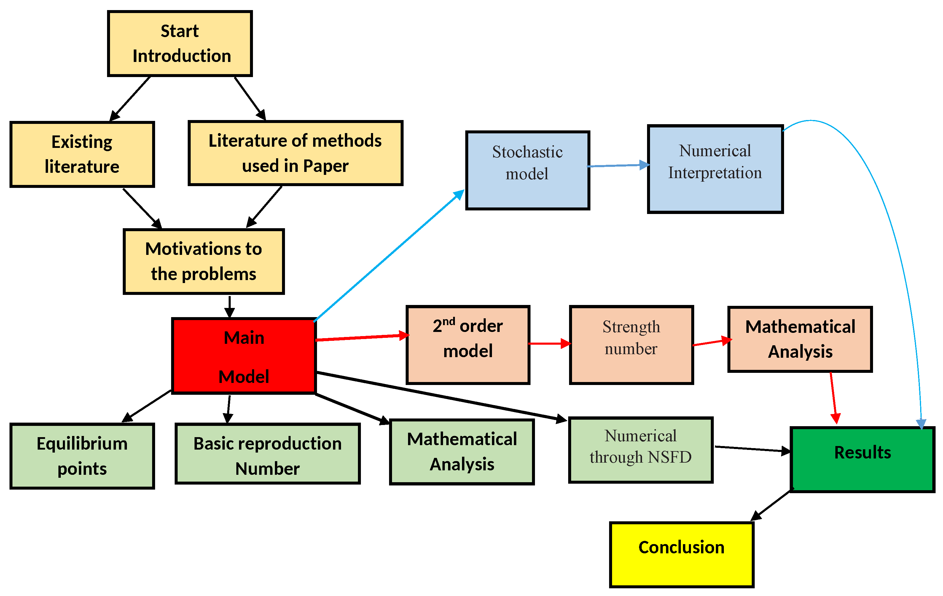
1. Introduction
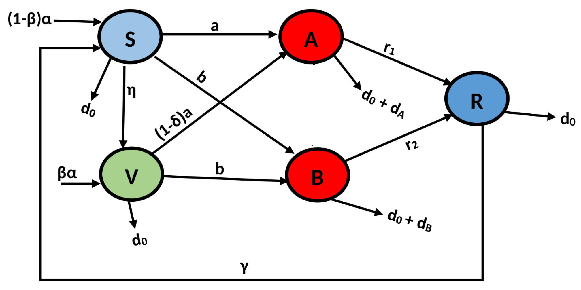
Model Formulation
2. Fundamental Analysis
3. Uniqueness and Existence
4. Mathematical Analysis of Deterministic Model
4.1. Disease-Free Equilibrium Points
4.2. Endemic Equilibrium
4.3. Expression for
- (i)
- If or/and , then there is no positive equilibrium.
- (ii)
- If or/and There exists a unique positive equilibrium called the endemic equilibrium.
5. Stability Analysis
5.1. Local Stability
5.2. Global Stability
- 1.
- A unique single variant of the delta infection equilibrium if and only if .
- 2.
- A unique single variant of the omicron infection equilibrium if and only if .
- 3.
- A double infection equilibrium when .
6. Second-Order Derivative Model
6.1. Strength Number
6.2. Mathematical Analysis
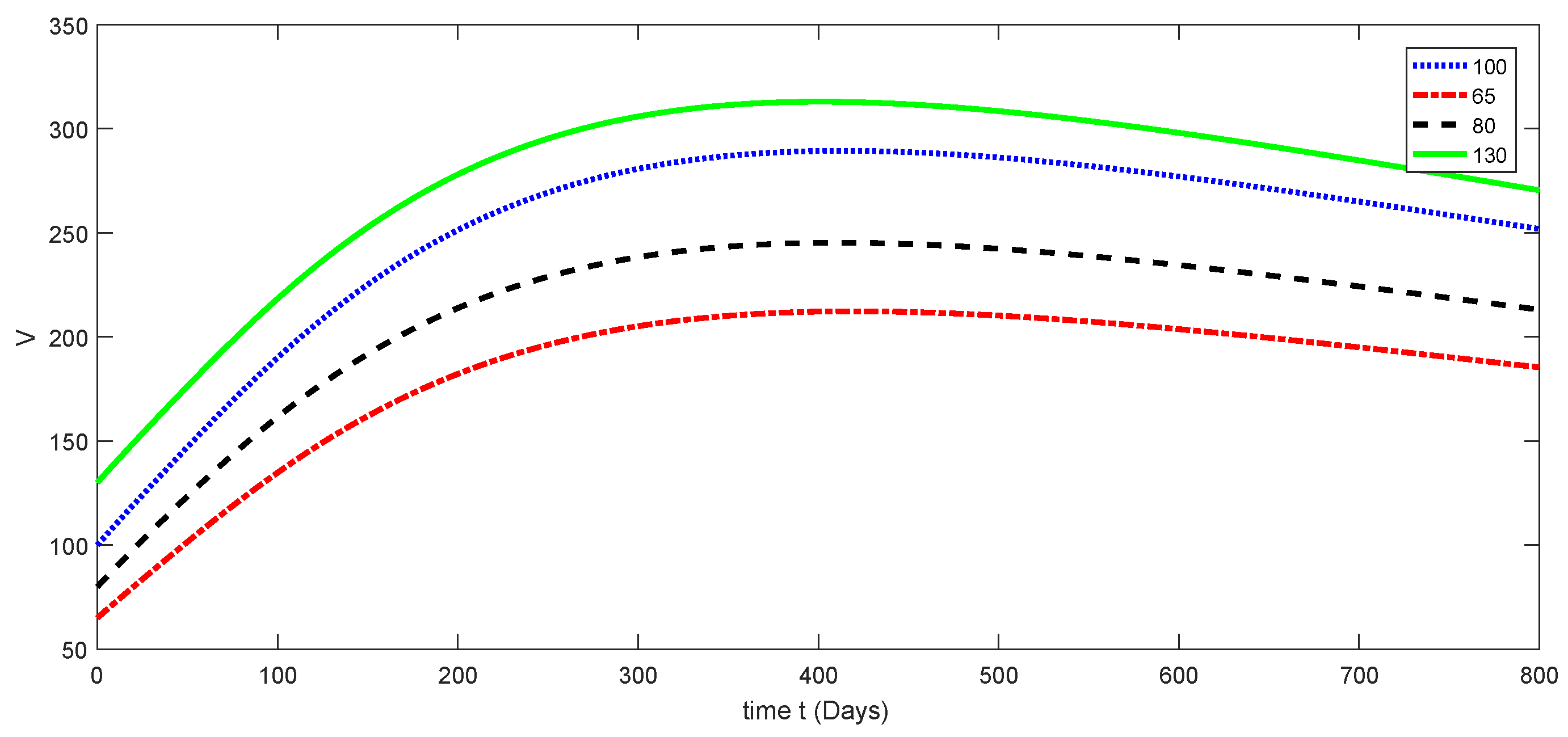
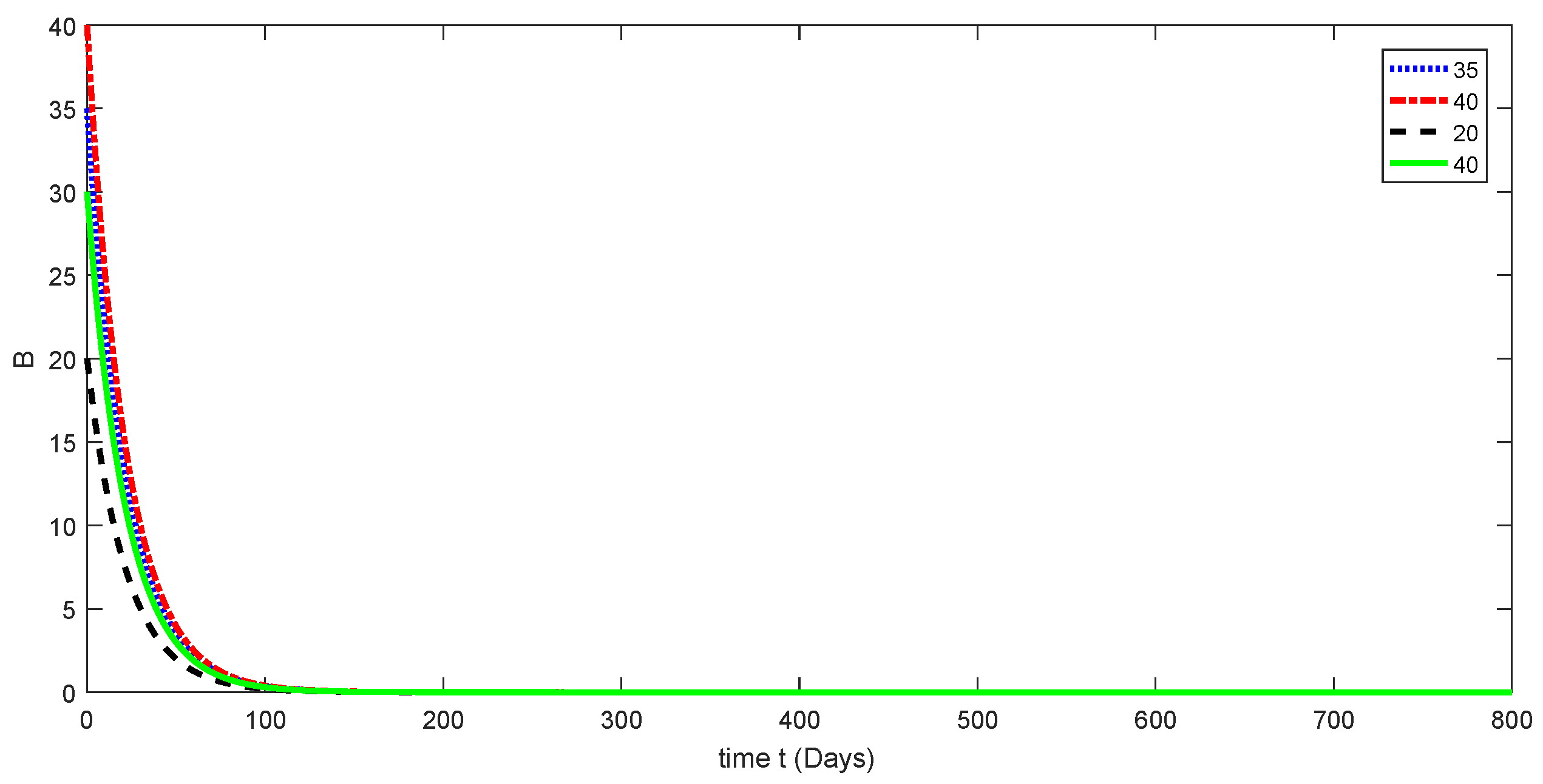
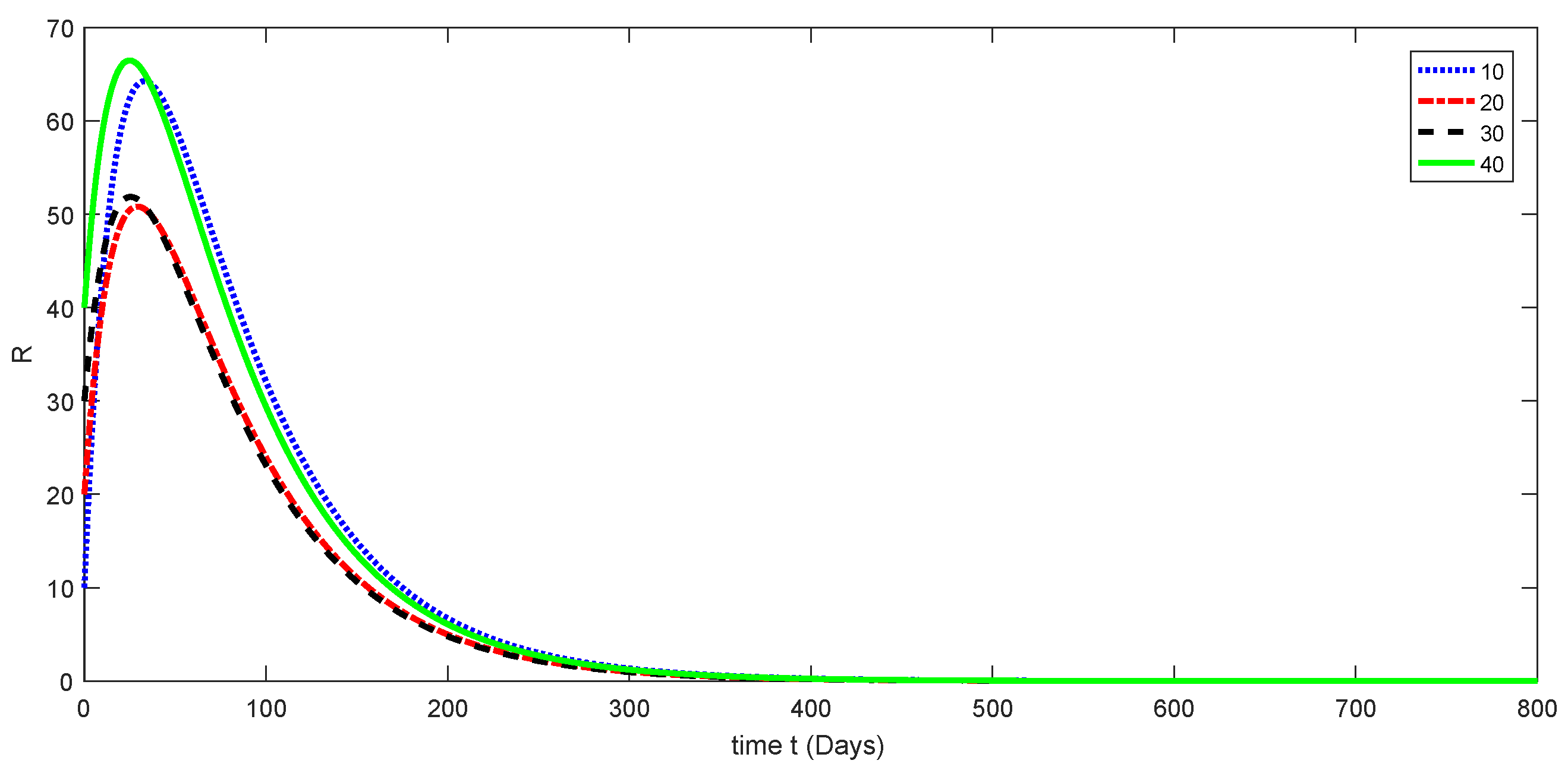
7. Numerical Results and Discussion for Deterministic Model
8. Stochastic form of the Proposed Model
Existence and Uniqueness of (23)
- (i)
- (ii)
- then
9. Basic Reproduction Number for Stochastic Model
10. Stability Analysis of Stochastic Model
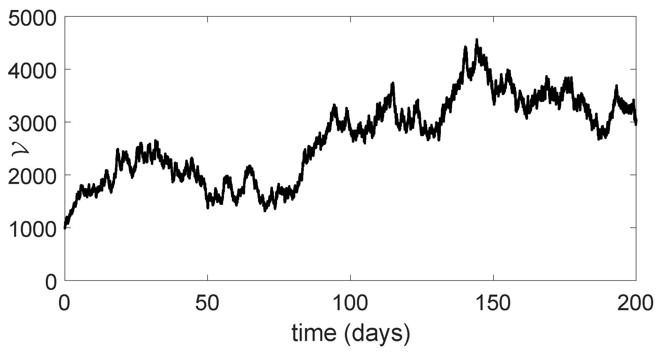
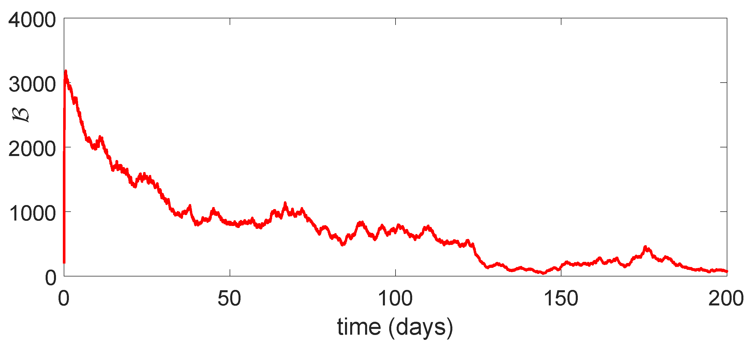
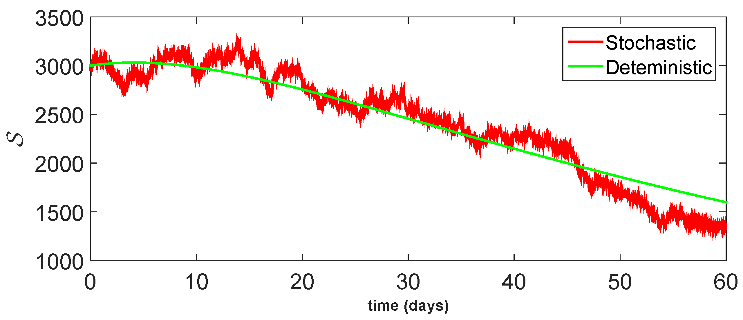
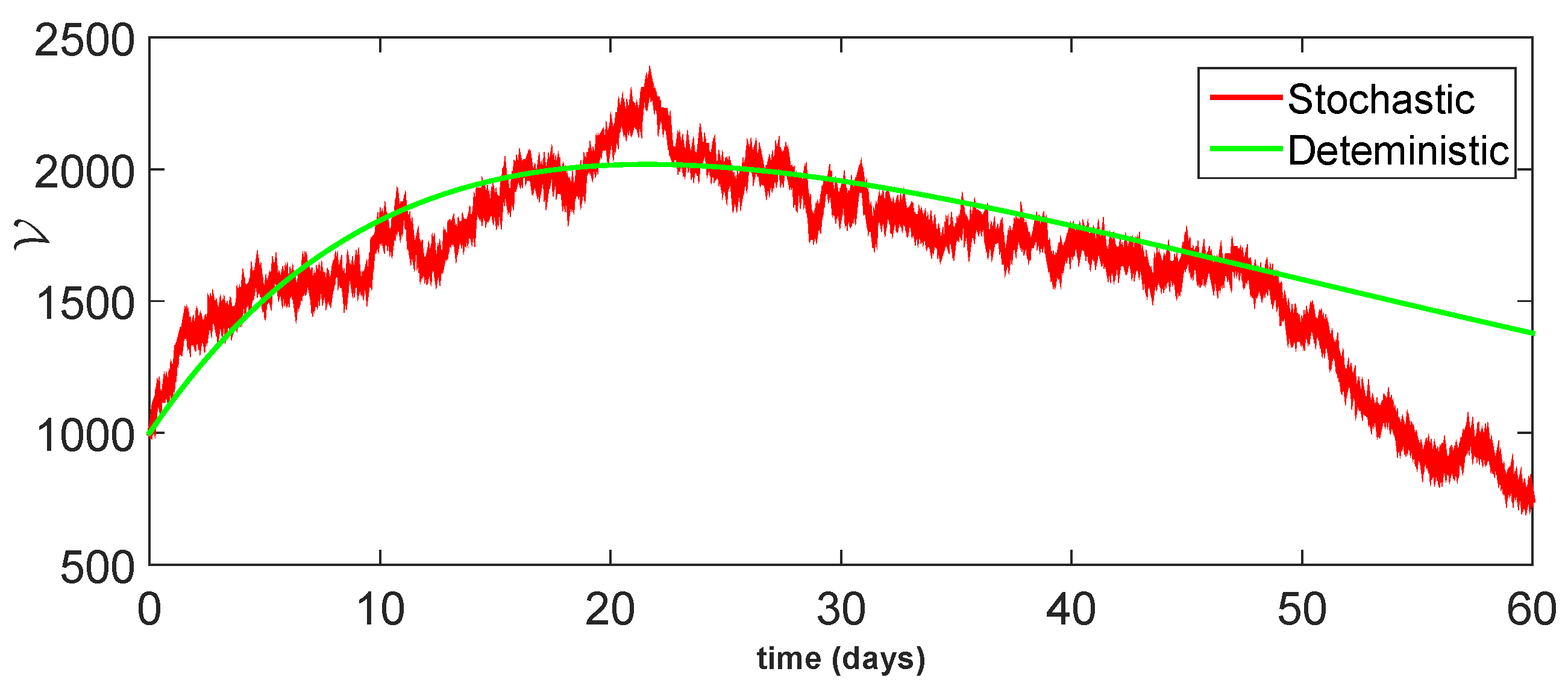
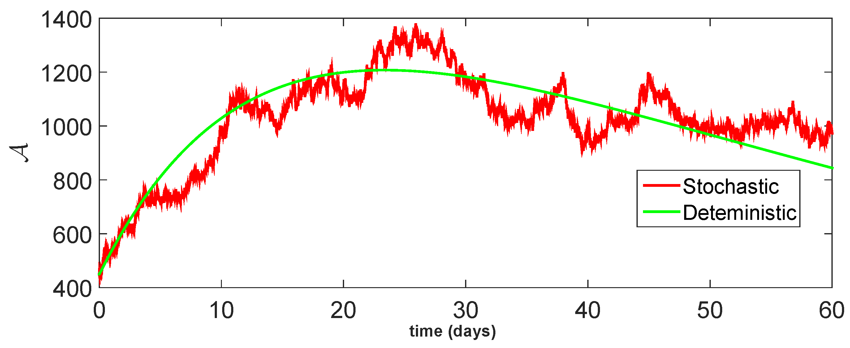
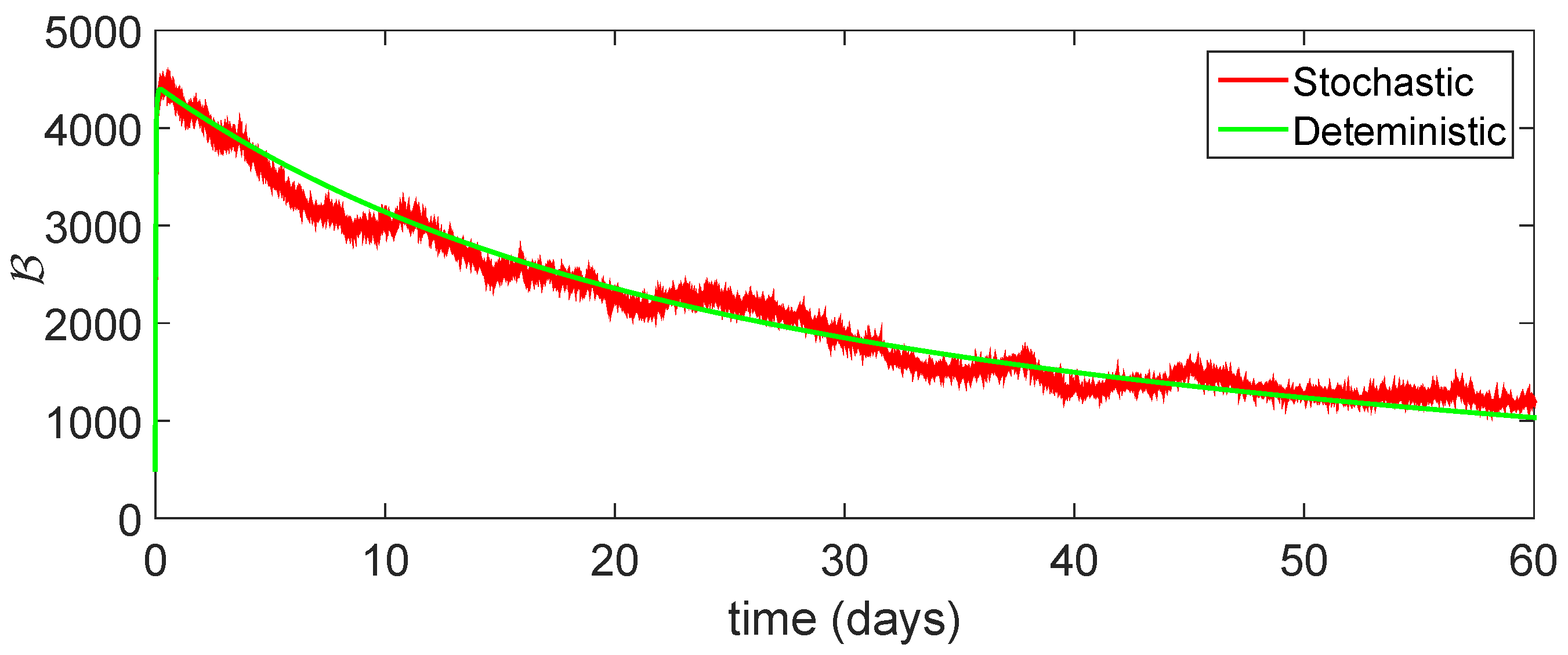
11. Stochastic Model and Numerical Interpretation
12. Conclusions
Author Contributions
Funding
Data Availability Statement
Acknowledgments
Conflicts of Interest
References
- Menachery, V.D., Jr.; Yount, B.L.; Debbink, K.; Agnihothram, S.; Gralinski, L.E.; Plante, J.A.; Graham, R.L.; Scobey, T.; Ge, X.-Y.; Donaldson, E.F.; et al. A SARS-like cluster of circulating bat coronaviruses shows potential for human emergence. Nat. Med. 2015, 21, 1508. [Google Scholar] [CrossRef]
- World Health Organization. Coronavirus Disease 2019 (COVID-19) Situation Report, 67; World Health Organization: Geneva, Switzerland, 2020. [Google Scholar]
- Li, Q.; Guan, X.; Wu, P.; Wang, X.; Zhou, L.; Tong, Y.; Ren, R.; Kathy, S.M.; Eric, H.Y.; Wong, J.Y.; et al. Early transmission dynamics in Wuhan, China, of novel coronavirus-infected pneumonia. N. Engl. J. Med. 2020, 382, 1199–1207. [Google Scholar] [CrossRef] [PubMed]
- World Health Organization. Coronavirus Disease 2019 (COVID-19): Situation Report, 72; World Health Organization: Geneva, Switzerland, 2020. [Google Scholar]
- Wu, Z.; McGoogan, J.M. Characteristics of and important lessons from the coronavirus disease 2019 (COVID-19) outbreak in china: Summary of a report of 72 314 cases from the Chinese center for disease control and prevention. JAMA 2020, 323, 1239–1242. [Google Scholar] [CrossRef] [PubMed]
- Gumel, A.B.; Iboi, E.A.; Ngonghala, C.N.; Elbasha, E.H. A primer on using mathematics to understand COVID-19 dynamics: Modeling, analysis and simulations. Inf. Dis. Mod. 2020, 6, 148–168. [Google Scholar] [CrossRef] [PubMed]
- Ewah, P.A.; Oyeyemi, A.Y.; Oyeyemi, A.L.; Oghumu, S.N.; Awhen, P.A.; Ogaga, M.; Edet, L.I. Comparison of exercise and physical activity routine and health status among apparently healthy Nigerian adults before and during COVID-19 lockdown: A self-report by social media users. Bull. Natl. Res. Cent. 2022, 46, 155. [Google Scholar] [CrossRef] [PubMed]
- Al-Raeei, M. The forecasting of COVID-19 with mortality using SIRD epidemic model for the United States, Russia, China, and the Syrian Arab Republic. AIP Adv. 2020, 10, 065325. [Google Scholar] [CrossRef]
- Olivares, A.; Staffetti, E. Uncertainty quantification of a mathematical model of COVID-19 transmission dynamics with mass vaccination strategy. Chaos Solitons Fractals 2021, 146, 110895. [Google Scholar] [CrossRef] [PubMed]
- Bala, S.; Gimba, B. Global sensitivity analysis to study the impacts of bed-nets, drug treatment, and their efficacies on a two-strain malaria model. Math. Comput. Appl. 2019, 24, 32. [Google Scholar] [CrossRef]
- Chung, K.W.; Lui, R. Dynamics of two-strain influenza model with cross-immunity and no quarantine class. J. Math. Biol. 2016, 73, 1467–1489. [Google Scholar] [CrossRef]
- Olayiwola, M.O.; Adedokun, K.A. A novel tuberculosis model incorporating a Caputo fractional derivative and treatment effect via the homotopy perturbation method. Bull. Natl. Res. Cent. 2023, 47, 121. [Google Scholar] [CrossRef]
- Chamchod, F.; Britton, N.F. On the dynamics of a two-strain influenza model with isolation. Math. Model. Nat. Phenom. 2012, 7, 49–61. [Google Scholar] [CrossRef]
- Rashkov, P.; Kooi, B.W. Complexity of host-vector dynamics in a two-strain dengue model. J. Biol. Dyn. 2021, 15, 35–72. [Google Scholar] [CrossRef] [PubMed]
- Li, X.Z.; Liu, J.X.; Martcheva, M. An age-structured two-strain epidemic model with super-infection. Math. Biosci. Eng. 2010, 7, 123–147. [Google Scholar] [PubMed]
- Ashrafur Rahman, S.M.; Zou, X. Flu epidemics: A two-strain flu model with a single vaccination. J. Biol. Dyn. 2011, 5, 376–390. [Google Scholar] [CrossRef]
- Allen, L.; Langlais, M.; Phillips, C.J. The dynamics of two viral infections in a single host population with applications to hantavirus. Math. Biosci. 2003, 186, 191–217. [Google Scholar] [CrossRef] [PubMed]
- Nuno, M.; Chowell, G.; Wang, X.; Castillo-Chavez, C. On the role of cross-immunity and vaccines on the survival of less fit flu strains. Theor. Popul. Biol. 2007, 71, 20–29. [Google Scholar] [CrossRef] [PubMed]
- Lazebnik, T.; Bunimovich-Mendrazitsky, S. Generic approach for mathematical model of multi-strain pandemics. PLoS ONE 2022, 17, e0260683. [Google Scholar] [CrossRef] [PubMed]
- Yagan, O.; Sridhar, A.; Eletreby, R.; Levin, S.; Plotkin, J.B.; Poor, H.V. Modeling and analysis of the spread of COVID-19 under a multiple-strain model with mutations. Harv. Data Sci. Rev. 2021, 4. [Google Scholar] [CrossRef]
- Massard, M.; Eftimie, R.; Perasso, A.; Saussereau, B. A multi-strain epidemic model for COVID-19 with infected and asymptomatic cases: Application to french data. J. Theoret. Biol. 2022, 545, 111117. [Google Scholar] [CrossRef]
- Atangana, A. Modelling the spread of COVID-19 with new fractal-fractional operators: Can the lockdown save mankind before vaccination? Chaos Solitons Fractals 2020, 136, 109860. [Google Scholar] [CrossRef]
- Lou, Y.; Salako, R.B. Control strategies for a multi-strain epidemic model. Bull. Math. Biol. 2022, 84, 10. [Google Scholar] [CrossRef] [PubMed]
- Puga, G.F.; Monteiro, L.H.A. The co-circulation of two infectious diseases and the impact of vaccination against one of them. Ecol. Complex. 2021, 47, 100941. [Google Scholar] [CrossRef]
- Shah, K.; Abdeljawad, T. Study of a mathematical model of COVID-19 outbreak using some advanced analysis. Waves Random Complex Media 2022, 2022, 1–18. [Google Scholar] [CrossRef]
- Ahmad, S.; Ullah, A.; Al-Mdallal, Q.M.; Khan, H.; Shah, K.; Khan, A. Fractional order mathematical modeling of COVID-19 transmission. Chaos Solitons Fractals 2020, 139, 110256. [Google Scholar] [CrossRef] [PubMed]
- Tchoumi, S.Y.; Rwezaura, H.; Tchuenche, J.M. Dynamic of a two-strain COVID-19 model with vaccination. Results Phys. 2022, 39, 105777. [Google Scholar] [CrossRef] [PubMed]
- Rwezaura, H.; Mtisi, E.; Tchuenche, J.M. A mathematical analysis of influenza with treatment and vaccination. Infect. Dis. Model. Res. Prog. 2010, 2010, 31–84. [Google Scholar]
- Van den Diressche, P.; Watmough, J. Reproduction number and sub threshold equilibria for compartmental models of disease transmission. Math. Biosci. 2002, 180, 29–48. [Google Scholar] [CrossRef]
- Khan, M.A.; Atangana, A. Modeling the dynamics of novel coronavirus (2019-nCov) with fractional derivative. Alex. Eng. J. 2020, 59, 2379–2389. [Google Scholar] [CrossRef]
- Gonzalez-Parra, G.; Martínez-Rodríguez, D.; Villanueva-Micó, R.J. Impact of a new SARS-CoV-2 variant on the population: A mathematical modeling approach. Math. Comput. Appl. 2021, 26, 25. [Google Scholar] [CrossRef]
- Pilishvili, T. Interim estimates of vaccine effectiveness of Pfizer-BioNTech and Moderna COVID-19 vaccines among health care personnel-33 US sites, January-March 2021. MMWR. Morb. Mortal. Wkly. Rep. 2021, 70, 753–758. [Google Scholar] [CrossRef]
- Tesfaye, A.W.; Satana, T.S. Stochastic model of the transmission dynamics of COVID-19 pandemic. Adv. Differ. Equ. 2021, 2021, 457. [Google Scholar] [CrossRef] [PubMed]


| Parameters | Physical Meaning and Representation |
|---|---|
| Susceptible compartment | |
| Vaccinated compartment | |
| Delta virus infected compartment | |
| Omicron virus infected compartment | |
| Recovered compartment | |
| Birth rate | |
| Disease death rate of delta virus | |
| Natural death rate | |
| Disease death rate of omicron virus | |
| Vaccination rate | |
| k | Contact rate |
| Transmission of delta virus | |
| Transmission of omicron virus | |
| Delta virus vaccine efficacy | |
| Loss of immunity | |
| Vaccination rate | |
| Recovery from delta virus | |
| Recovery of omicron virus |
| Parameters | Approximate Values [31,32] |
|---|---|
| 0.0016 | |
| 0.0000683 | |
| 0.0032 | |
| 0.0032 | |
| 0.011 | |
| k | 0.024 |
| 0.127 | |
| 0.127 | |
| 0.16 | |
| 0.01111 | |
| 0.09 | |
| 0.09 | |
| 0.09 |
| Error Analysis | ||
|---|---|---|
| Compartment | Error of Approximation for Deterministic Model | Error of Approximation for Stochastic Model |
| 0.05432 | 0.00345 | |
| 0.03214 | 0.008765 | |
| 0.01236 | 0.001129 | |
| 0.06754 | 0.003214 | |
| 0.00769 | 0.000341 | |
Disclaimer/Publisher’s Note: The statements, opinions and data contained in all publications are solely those of the individual author(s) and contributor(s) and not of MDPI and/or the editor(s). MDPI and/or the editor(s) disclaim responsibility for any injury to people or property resulting from any ideas, methods, instructions or products referred to in the content. |
© 2024 by the authors. Licensee MDPI, Basel, Switzerland. This article is an open access article distributed under the terms and conditions of the Creative Commons Attribution (CC BY) license (https://creativecommons.org/licenses/by/4.0/).
Share and Cite
Jeelani, M.B.; Din, R.U.; Alhamzi, G.; Hleili, M.; Alrabaiah, H. Deterministic and Stochastic Nonlinear Model for Transmission Dynamics of COVID-19 with Vaccinations Following Bayesian-Type Procedure. Mathematics 2024, 12, 1662. https://doi.org/10.3390/math12111662
Jeelani MB, Din RU, Alhamzi G, Hleili M, Alrabaiah H. Deterministic and Stochastic Nonlinear Model for Transmission Dynamics of COVID-19 with Vaccinations Following Bayesian-Type Procedure. Mathematics. 2024; 12(11):1662. https://doi.org/10.3390/math12111662
Chicago/Turabian StyleJeelani, Mohammadi Begum, Rahim Ud Din, Ghaliah Alhamzi, Manel Hleili, and Hussam Alrabaiah. 2024. "Deterministic and Stochastic Nonlinear Model for Transmission Dynamics of COVID-19 with Vaccinations Following Bayesian-Type Procedure" Mathematics 12, no. 11: 1662. https://doi.org/10.3390/math12111662
APA StyleJeelani, M. B., Din, R. U., Alhamzi, G., Hleili, M., & Alrabaiah, H. (2024). Deterministic and Stochastic Nonlinear Model for Transmission Dynamics of COVID-19 with Vaccinations Following Bayesian-Type Procedure. Mathematics, 12(11), 1662. https://doi.org/10.3390/math12111662