Convolutional Neural Networks for Local Component Number Estimation from Time–Frequency Distributions of Multicomponent Nonstationary Signals

Abstract

Frequency-modulated (FM) signals, prevalent across various applied disciplines, exhibit time-dependent frequencies and a multicomponent nature necessitating the utilization of time-frequency methods. Accurately determining the number of components in such signals is crucial for various applications reliant on this metric. However, this poses a challenge, particularly amidst interfering components of varying amplitudes in noisy environments. While the localized Rényi entropy (LRE) method is effective for component counting, its accuracy significantly diminishes when analyzing signals with intersecting components, components that deviate from the time axis, and components with different amplitudes. This paper addresses these limitations and proposes a convolutional neural network-based (CNN) approach for determining the local number of components using a time–frequency distribution of a signal as input. A comprehensive training set comprising single and multicomponent linear and quadratic FM components with diverse time and frequency supports has been constructed, emphasizing special cases of noisy signals with intersecting components and differing amplitudes. The results demonstrate that the estimated component numbers outperform those obtained using the LRE method for considered noisy multicomponent synthetic signals. Furthermore, we validate the efficacy of the proposed CNN approach on real-world gravitational and electroencephalogram signals, underscoring its robustness and applicability across different signal types and conditions.

1. Introduction

In various scientific domains, such as gravitational wave detection [1], radar systems [2,3], tire sensor signal processing [4] and biomedical signal processing [5,6], signals frequently exhibit nonlinear frequency modulation (FM), characterized by time-dependent frequencies known as instantaneous frequencies (IFs). Time–frequency distributions (TFDs) are essential tools for representing signal energy in the joint time–frequency (TF) domain [7]. Quadratic TFDs (QTFDs), widely utilized in practical contexts, frequently yield undesirable oscillatory artifacts, referred to as cross-terms, notably evident in signals comprising multiple components. While methods such as two-dimensional (2D) low-pass filters in the ambiguity function (AF) can suppress cross-terms, they may compromise the quality of useful components, known as auto-terms. Given the diversity of signals, various TFD methods have emerged over time [7,8,9,10].

Many methods in time–frequency signal analysis, such as IF estimation methods, signal decomposition, and TFD reconstruction methods, necessitate prior knowledge of the local number of signal components, i.e., signal complexity [7,11,12,13,14]. Traditionally, global concentration and entropy measures are employed on a whole TFD to assess global signal complexity [7]. However, to assess local changes of signal complexity, the authors in [15,16] proposed the localized version of the Rényi entropy, namely the localized Rényi entropy (LRE), which estimates the local number of components for a given TFD. Given that the original LRE has been implemented over time slices of a TFD, it has been also named as the short-term Rényi entropy (STRE) [15,16]. This approach does not require any prior knowledge about the signal, making it applicable to signals with different FM components. The information about the local number of components has found utility in several applications, including image-based and blind source separation algorithms for IF estimation [6], QTFD optimization [17], sparse TFD reconstruction [18,19,20,21,22,23] and signal denoising [24,25], to name a few.

Despite many applications and advantages, the LRE suffers from several drawbacks. Firstly, experiments confirm the method’s limitation when signal components overlap [15,16,26]. Secondly, the LRE may fail to recognize components with very low amplitudes, prompting the proposal of an iterative approach to enhance detection accuracy [27]. Thirdly, constant reference signal requirements are not suitable when observed signal components deviate from the time axis, necessitating localization via frequency slices [18,19,22]. Consequently, the authors in [18,19] proposed the usage of the narrow-band Rényi entropy (NBRE), which should be used alongside the STRE in TFD reconstruction methods. Finally, the authors in [22] additionally emphasized the requirement of the usage of both, the STRE and NBRE, in IF estimation algorithms, and proposed a method that divides TFD into segments that require different localization and specific LRE approach.

However, these challenges are not entirely solved within a single method. The main advantages and disadvantages of all three versions of the LRE are given in

Table 1. Comparison of LRE versions: original STRE, Iterative LRE, and NBRE.

LRE Version	Advantages	Disadvantages
Original (STRE) [15,16]	1. Used in many applications 2. Robust against noise	1. Limited by overlapping components 2. Struggles with low amplitudes 3. Constant reference signal unsuitable for certain signal components
Iterative LRE [27]	Detects components with lower amplitudes	1. Sensitive to noise 2. Less effective for close or intersecting components 3. Emphasizes unresolved interference terms
NBRE [18,19]	1. Provides number of local components in frequency slices 2. More suitable than STRE for certain signal components	Same limitations as STRE

. Additionally, the combined usage of the STRE and NBRE requires careful user inspection of the signal’s TFD, or an additional method mentioned above [22], which can be time-consuming and imprecise for components at and in the vicinity of their intersection. Additionally, it is noteworthy that both the STRE and NBRE may yield inaccuracies when applied to multicomponent signals exhibiting diverse component characteristics, thereby underscoring the imperative for the development of a unified approach.

This study aims to address the aforementioned limitations by proposing an effective method for local component counting in TFDs through the utilization of convolutional neural networks (CNNs). CNNs have demonstrated considerable potential across various applications, particularly in time–frequency signal analysis. Shang et al. [28] demonstrate the application of a CNN-LSTM hybrid network for signal processing ultrasonic guided lamb waves, to detect damage, corrosion, or welding defects in the metallic pipelines. Authors reach an accuracy of up to 94.8%, showing high performance, especially on higher signal-to-noise ratios. CNNs have also been applied on the scalogram images by Zaman et al. [29], to detect and diagnose faults in the operation of centrifugal pumps. Authors demonstrate an improvement in accuracy of 14% above the state-of-the-art score. Applications on spectrogram images are not uncommon—Patil et al. [30] demonstrate the application of CNNs architectures trained on vibration spectrograms to determine the health of milling tool inserts. They use the pre-defined CNNs, such as VGG16, and achieve accuracies of approximately 98%. A similar approach is used by Jung et al. [31], with spectrograms of sound-based data, coming from the engine used to detect faults in the rotor. Authors apply CNNs with transfer learning on the spectrograms produced with STFT, gaining models with accuracy above 99%. These examples demonstrate the high applicability of CNNs on images generated with time–frequency analysis.

In this research, our goal is to demonstrate that training datasets for the proposed CNN can be constructed from synthetic single and multicomponent signals, encompassing both linear FM (LFM) and quadratic FM (QFM) components, to achieve improvements over the LRE method and robust performance across a wide spectrum of signals. Special emphasis is placed on signal scenarios featuring diverse time and frequency supports, closely spaced and intersecting components, and variations in component amplitudes, where existing methods have exhibited significantly diminished accuracy. We also show that incorporating additive white Gaussian noise (AWGN) into the training process reduces the CNN’s sensitivity to noise. This approach allows users to simply provide the signal’s TFD, eliminating the need for additional parameter tuning or the use of additional LRE variants and component separation techniques. In addition to the synthetic signal examples, our study demonstrates the enhanced accuracy of estimated local numbers of components for real-world electroencephalogram (EEG) and gravitational signal examples, previously unseen by CNN. The key contributions of this study are summarized as follows:

• Development of a novel CNN-based framework for accurate local component counting in TFDs, overcoming the limitations of traditional LRE methods.
• Introduction of a comprehensive training dataset comprising synthetic signals with LFM and QFM components, facilitating the robust generalization of the CNN across a wide range of synthetic and real-world signal types and complexities.
• Incorporation of AWGN into the training process, improving the CNN’s robustness to noise.
• Simplification of the local component counting process by eliminating the need for additional parameter tuning within the LRE method and the use of additional iterative LRE and NBRE approaches, streamlining the application for end-users.

The remainder of the paper is structured as follows. Section 2.1 introduces adaptive time–frequency distributions. Section 2.2 defines the LRE method and highlights its limitations. The methodology of the proposed CNN is outlined in Section 2.3. Section 3 presents the experimental simulation results and provides a discussion. Finally, Section 4 presents the conclusions of the paper.

2. Materials and Methods

2.1. Adaptive Time–Frequency Distributions

The representation of a nonstationary signal comprising $NC$ components, denoted as $z\left(t\right)$, is established as the analytical counterpart of a real signal, delineated as [7]

$$z\left(t\right)=\sum _{k=1}^{NC}{z}_k\left(t\right)=\sum _{k=1}^{NC}{A}_k\left(t\right)e^{j{\phi }_k\left(t\right)},$$

(1)

where $z_k\left(t\right)$ is the k-th signal component, while $A_k\left(t\right)$ and ${\phi }_k\left(t\right)$ denote the k-th signal component’s instantaneous amplitude and phase, respectively.

The ideal TFD, denoted as $\hat{\mathrm{Y}}(t,f)$, assumes the form of a unit delta function that traces the crests of ridges representing the IF, $f_{0_k}\left(t\right)$, for each component. This concept is articulated as [7]

$$\hat{\mathrm{Y}}(t,f)=\sum _{k=1}^{NC}{A}_k^2\left(t\right)\delta (f-f_{0_k}\left(t\right)),$$

(2)

$$f_{0_k}\left(t\right)=\frac{1}{2\pi }\frac{d}{dt}argz\left(t\right)=\frac{1}{2\pi }\frac{d{\phi }_k\left(t\right)}{dt},$$

(3)

where $f_{0_k}\left(t\right)$ signifies the dominant frequency of the k-th component at a specific time. However, achieving the ideal TFD is often unattainable due to the imprecise localization and potential influence of cross-terms in practical scenarios, as acknowledged in the literature [7].

The Wigner–Ville distribution (WVD) stands as a core TFD method, offering a near-perfect estimate of IF for signals dominated by a single LFM component in the TF plane [7]. The WVD is defined as the Fourier transform (FT) of the instantaneous auto-correlation function (IACF) $R_z(t,\tau )=z\left(t+\frac{\tau }{2}\right)z^{\ast }\left(t-\frac{\tau }{2}\right)$ as [7]

$$W{V}_z(t,f)={\int }_{-\infty }^{\infty }{R}_z(t,\tau )e^{-j2\pi f\tau }d\tau .$$

(4)

Despite its efficacy, the susceptibility to cross-terms in multicomponent signals necessitates effective suppression techniques. Utilizing the AF, denoted as $A_F(\nu ,\tau )$ [7]

$$A_F(\nu ,\tau )={\int }_{-\infty }^{\infty }{\int }_{-\infty }^{\infty }W{V}_z(t,f)e^{j2\pi (f\tau -\nu t)}dtdf,$$

(5)

and a 2D low-pass filter, denoted with $w(\nu ,\tau )$

$${\mathcal{A}}_F(\nu ,\tau )=A_F(\nu ,\tau )w(\nu ,\tau ),$$

(6)

$$\mathrm{Y}(t,f)={\int }_{-\infty }^{\infty }{\int }_{-\infty }^{\infty }{\mathcal{A}}_F(\nu ,\tau )e^{-j2\pi (f\tau -\nu t)}d\nu d\tau ,$$

(7)

offers a pathway to define a class of TFDs known as QTFDs, represented by $\mathrm{Y}(t,f)$ [7]. Usually, simple multiplication in the AF is computationally less demanding than using double convolution, denoted with double asterisk ∗, in the TF domain as [7]

$$\mathrm{Y}(t,f)=g\left(t\right)\underset{t}{\ast }H\left(f\right)\underset{f}{\ast }W{V}_z(t,f)=W{V}_z(t,f)\underset{t}{\ast }\underset{f}{\ast }\gamma (t,f),$$

(8)

where $\gamma (t,f)$ denotes the separable kernel for smoothing the WVD in the TF domain. One of such TFDs using the independent smoothing kernels is the smoothed-pseudo Wigner–Ville distribution (SPWV), defined as [7]

$$SPW{V}_z(t,f)={\int }_{-\infty }^{\infty }h\left(\tau \right){\int }_{-\infty }^{\infty }g(u-t)z\left(u+\frac{\tau }{2}\right)·z^{\ast }\left(u-\frac{\tau }{2}\right)du{e}^{-j2\pi f\tau }d\tau .$$

(9)

QTFDs aim to strike a balance between concentrating autoterms and attenuating cross-terms, a challenge well-documented in the literature [7].

To address the limitations of conventional TFDs, an approach called the adaptive directional TFD (ADTFD) is introduced, as outlined by [14,32]. For each point in the TF plane, this technique adapts the direction of the kernel ${\gamma }_{\theta }(t,f)$, expressed as

$${\mathrm{Y}}_{\left(a\right)}(t,f)=\mathrm{Y}(t,f)\underset{t}{\ast }\underset{f}{\ast }{\gamma }_{\theta }(t,f),$$

(10)

where ${\gamma }_{\theta }(t,f)$ represents the smoothing kernel controlled by $\theta$ [14,32]. In our research, we utilized the extended modified B distribution (EMB) as the basis QTFD, with its $w\left(\nu ,\tau \right)$ separable kernel defined according to the established parameters [7]

$$w\left(\nu ,\tau \right)=\frac{{\int }_{-\infty }^{\infty }{\cos \mathrm{h}}^{-2{\beta }_{EMB}}\left(t\right)e^{j2\pi \nu t}dt}{{\int }_{-\infty }^{\infty }{\cos \mathrm{h}}^{-2{\beta }_{EMB}}\left(t\right)dt}{\cos \mathrm{h}}^{-2{\alpha }_{EMB}}\left(\tau \right),$$

(11)

where ${\alpha }_{EMB}={\beta }_{EMB}=0.25$ serve as the smoothing parameters in time and frequency as in [14,32,33,34]. The chosen smoothing kernel, ${\gamma }_{\theta }(t,f)$, is the double-derivative directional Gaussian filter (DGF), as introduced in previous studies [14,32,33,34]:

$${\gamma }_{\theta }(t,f)=\frac{ab}{2\pi }\frac{d^2}{d{f}_{\theta }^2}{e}^{-a^2{t}_{\theta }^2-b^2{f}_{\theta }^2}.$$

(12)

The degree of smoothing along the time and frequency axes are regulated by the parameters a and b, respectively [14]. For each TF point, the orientation angle of ${\gamma }_{\theta }(t,f)$ is adjusted locally by maximizing the correlation with TF ridges as

$$\theta (t,f)=arg\underset{\theta }{max}\left|\left|\mathrm{Y}(t,f)\right|\underset{t}{\ast }\underset{f}{\ast }{\gamma }_{\theta }(t,f)\right|,$$

(13)

where $\theta \in [-\pi /2,\pi /2]$ [14].

The optimization of smoothing kernel parameters and shape is crucial for optimal performance and depends on the signal under analysis. Previous studies have suggested ranges for parameters a and b to balance the intensity of smoothing and prevent component merging. Additionally, the window length $WL$ affects the performance of ADTFD, with smaller values failing to resolve close components but preserving short-duration signals’ energy, and larger values achieving the opposite effect.

To automate parameter optimization, we employed the locally adaptive ADTFD (LOADTFD) method proposed by [33], which selects TF points with minimal values from a set of ADTFDs and their respective parameters. This results in a LOADTFD that effectively preserves short-duration signals’ energy while enhancing resolution and suppressing interference. In our study, we selected parameter values $(a,b)$ from a predefined set, while $WL$ was tuned for each combination of $(a,b)$ using the energy concentration measure [35]

$$M_z^S=\frac{1}{N_t{N}_f}{\left({\int }_{-\infty }^{\infty }{\int }_{-\infty }^{\infty }|{\displaystyle \frac{{\mathrm{Y}}_{\left(a\right)}(t,f)}{{\int }_{-\infty }^{\infty }{\int }_{-\infty }^{\infty }{\mathrm{Y}}_{\left(a\right)}dtdf}}{|}^{\frac{1}{2}}dtdf\right)}^2,$$

(14)

where $N_t$ and $N_f$ represent the numbers of time samples and frequency bins, respectively. For the pairs $(3,6)$ and $(2,20)$, the range is set to $[N_t/8:4:N_t/4]$, while for the pairs $(3,8)$ and $(2,30)$, it is set to $[N_t/4:4:3N_t/8]$, as suggested in prior work [33].

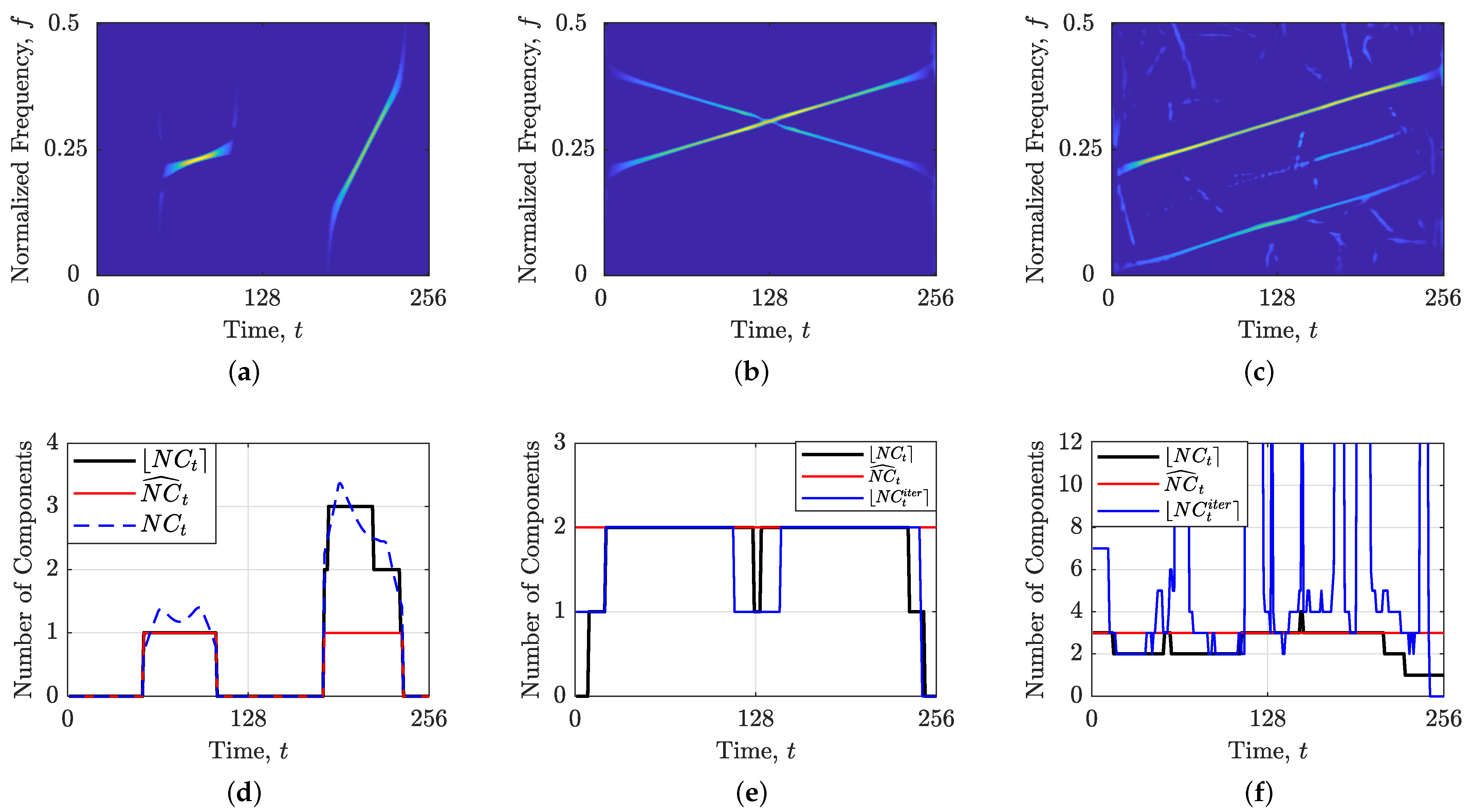
2.2. The Localized Rényi Entropy

Considering that TFD represents a pseudo-energy density in the TF domain, the Rényi entropy, represented as $H\left(\mathrm{Y}\right(t,f\left)\right)$, serves as a comprehensive measure of signal complexity in the TF domain [36,37,38]. It is defined by the expression

$$H\left(\mathrm{Y}(t,f)\right)={\displaystyle \frac{1}{1-{\alpha }_R}}{log}_2{\int }_{-\infty }^{\infty }{\int }_{-\infty }^{\infty }{\left({\displaystyle \frac{\mathrm{Y}(t,f)}{{\int }_{-\infty }^{\infty }{\int }_{-\infty }^{\infty }\mathrm{Y}(t,f)dtdf}}\right)}^{{\alpha }_R}dtdf,$$

(15)

where ${\alpha }_R>2\in \mathbb{N}$ is set as an odd integer to integrate out the cross-terms. As can be observed in (15), this is a global version of the measure, meaning that it is applied to a whole TFD. The primary constraint of the global Rényi entropy estimation approach is its applicability solely to multicomponent signals composed of shifted replicas of a single fundamental component. It proves ineffective when confronted with multicomponent signals featuring components with varying time/frequency supports and frequency modulations [15,16].

To address this challenge, the local number of signal components can be estimated by leveraging the counting characteristics of the Rényi entropy using a short-time moving window (controlled by the parameter ${\Theta }_t$) [15,16]. Termed the LRE or STRE, this complexity measure enables the continuous estimation of the number of components within the moving time window, given by [15,16]

$$N{C}_t\left(t_0\right)=2^{H\left({\mathrm{Y}}^{{\Delta }_{t_0}}(t,f)\right)-H\left({\mathrm{Y}}_{\mathrm{ref}}^{{\Delta }_{t_0}}(t,f)\right)},$$

(16)

where ${(·)}^{{\Delta }_{t_0}}$ denotes that only a segment of TFD in the vicinity of $t_0$ is considered

$${\mathrm{Y}}^{{\Delta }_{t_0}}(t,f)=\left\{\begin{array}{cc}\mathrm{Y}(t,f),\hfill & t\in [t_0-\frac{{\Theta }_t}{2},t_0+\frac{{\Theta }_t}{2}],\hfill \\ 0,\hfill & \mathrm{otherwise}.\hfill \end{array}\right.$$

(17)

Note that ${\mathrm{Y}}_{\mathrm{ref}}(t,f)$ denotes the TFD of a reference signal that is chosen as a cosine signal with an amplitude of 1 and a constant normalized frequency of 0.1 [15,16]. Even though time and frequency marginals are not preserved over short-term estimation intervals, it has been demonstrated that the counting property of the Rényi entropy remains valid under the assumption of a positive TFD and TFD with reduced interference [15,16].

Driven by the constraints of entropy-based estimation methods for signals with components of equal amplitudes, an iterative method for estimating the local number of components with varying spectral amplitudes was delineated [27]. In this strategy, the predominant spectral component is filtered out in each iteration, which consequently emphasizes weaker spectral components. At each iteration j of the algorithm, $N{C}_t^{\left[j\right]}\left(t\right)$ is computed. Subsequently, for time slices where $N{C}_t^{\left[j\right]}\left(t\right)\ge 1$, the counter $N{C}_t^{iter}\left(t\right)$ is incremented by 1, and the component with the highest amplitude is eliminated. The algorithm stops at the j-th iteration when $maxN{C}_t^{\left[j\right]}\left(t\right)\le 1$, indicating the absence of components identified by the entropy. The final value of $N{C}_t^{iter}\left(t\right)$ represents the estimated local number of components obtained by this iterative method [17,27].

Limitations

The limitations of both the original and iterative LRE methods are illustrated in Figure 1 using three synthetic signal instances featuring LFM components. The first signal example (see Figure 1a) portrays two LFM components with distinct slopes relative to the time axis. In Figure 1d, it is evident that as a signal component deviates considerably from the reference component of the LRE, the $N{C}_t$ experiences an artificial increase, leading to significantly inaccurate estimates compared to those for components more parallel to the time axis that are considerably closer to the ideal ${\widehat{NC}}_t$. This discrepancy arises from the calculation of the LRE in (16), where the Rényi entropy of the segmented single component becomes substantially larger than the reference ($H\left({\mathrm{Y}}^{{\Delta }_{t_0}}(t,f)\right)>>H\left({\mathrm{Y}}_{\mathbf{ref}}^{{\Delta }_{t_0}}(t,f)\right)$).

The second signal example depicted in Figure 1b showcases two intersecting LFM components. As depicted in Figure 1e, both the original $N{C}_t$ and iterative $N{C}_t^{iter}$ exhibit a decline when two components intersect. The limitation of the iterative method lies in the inadvertent removal of the strongest component, resulting in the unwanted deletion of the second component precisely at and near the intersection point. Consequently, this leads to an even larger decrease in the number of components as observed in the original LRE method.

The third signal instance, composed of three LFM components with different amplitudes (see Figure 1c), was embedded in strong AWGN with a signal-to-noise ratio (SNR) of 2 dB, demonstrating a limitation of the iterative LRE method wherein noise samples are erroneously recognized as auto-terms.

It is apparent that the iterative LRE approach does not effectively address the aforementioned limitations of the original approach, except in specific cases where components exhibit different amplitudes in a noise-free environment. Additionally, research in [6] demonstrates significant dependence of $N{C}_t^{iter}$ on the initial TFD threshold level when considering real-world EEG signals. The utility of the iterative LRE is better suited for purposes such as extracting the strongest component, as demonstrated in [6], and for optimization purposes where cross-terms need to be detected, interpreting $N{C}_t^{iter}$ as the number of total energy regions rather than the number of auto-terms [17]. Therefore, in this study, we opt to consider the original and more robust LRE method for comparison in Section 3, as has been widely utilized across various applications [11,18,19,20,21,22,39].

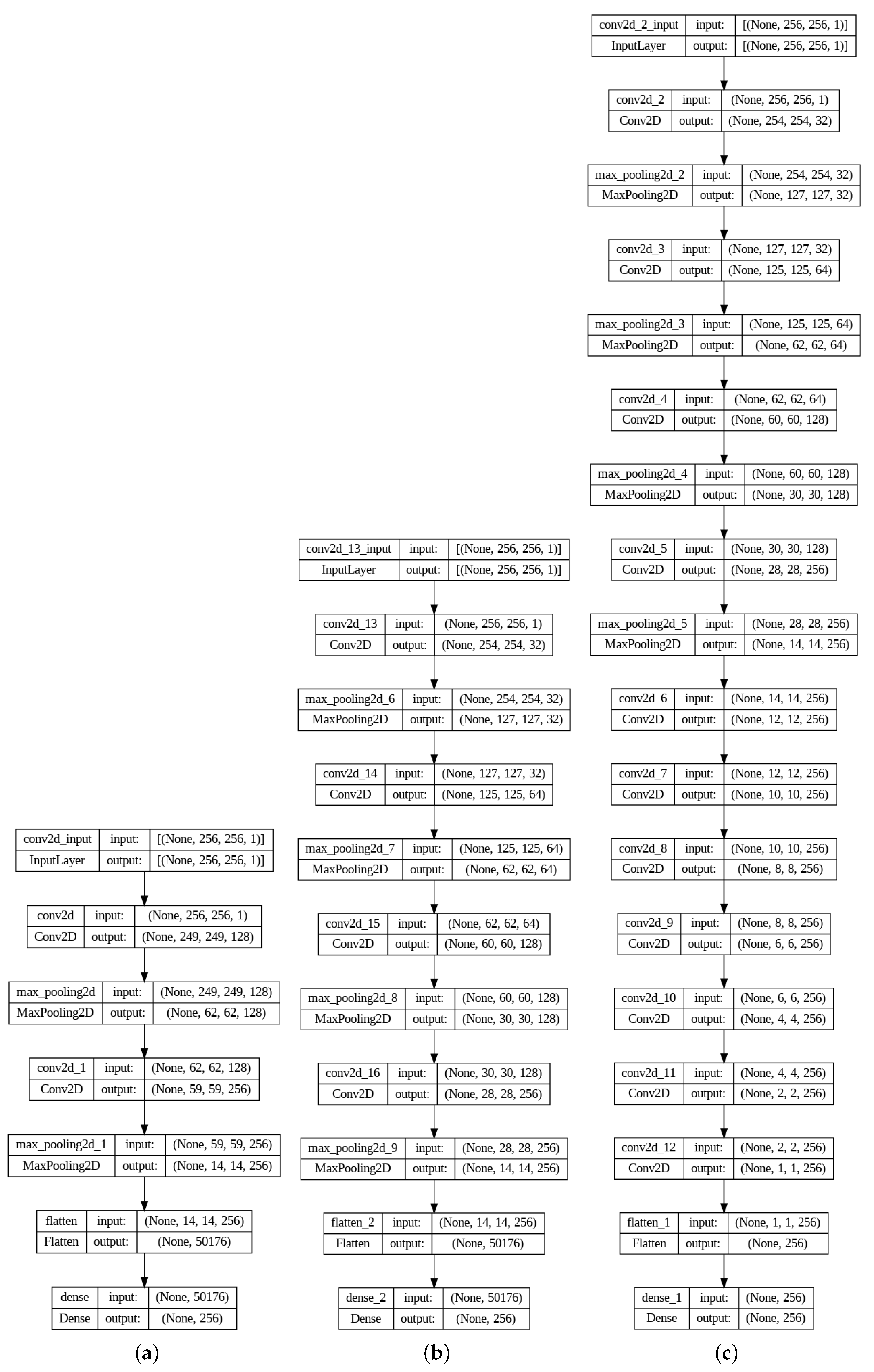
2.3. The Proposed CNN-Based Approach

Convolutional neural networks are based on the application of filters that are convoluted with the input of the network. In comparison to the classic artificial neural networks (ANNs), the network parameters are stored as the values within the filter tensors instead of within the connection weights between neurons [40]. The training process is the same as with the classic artificial neural networks—with the error determined in the forward propagation stage, and the filter values adjusted in the backward propagation stage, based on the error gradient [41].

When discussing the application of matrix-shaped two-dimensional data, the models commonly applied are the two-dimensional convolutional networks, built of layers that perform the two-dimensional convolution operation, per

$$(I\ast h)(m,n)=\sum _{u=-\infty }^{\infty }\sum _{v=-\infty }^{\infty }I(u,v)·h(m-u,n-v),$$

(18)

with the I being the input matrix, h being the applied filter, m and n being the indices of the feature map and u, v being the indices of the filter. In addition to the convolutional layers, another applied is the max pooling layer, which reduces the dimensionality of the input by selecting the maximum value from a subset of the input matrix. The pooling operation is defined as

$$(I\ast h)(m,n)=\underset{u,v}{max}I(m·s+u,n·s+v).$$

(19)

We define three different CNN architectures, with the main differentiation being the depth of the network—in other words, the amount of convolutional and pooling layers applied. To simulate the application of the previous methods and to generate the expected output of the number of components present in time, all the models are tuned to output a vector of 256 values, which is compared to the expected output, as described previously. Each convolutional layer is defined by its width and height. Due to them being the same for each example in this study, a choice is made based on the fact the input is square as well, the width and height are defined as a single value—N. Additionally, the number of filters k is another parameter, as each filter is applied to the input, allowing for the creation of more feature maps—or in other words, a greater amount of network parameters to be tuned. That way, each convolutional layer can be defined as $(k,(m,m\left)\right)$, with the max pooling layer defined as $(s,s)$, with s being the stride of the pooling operation. With that, the change in the dimensionality of the input can be calculated as, in the case of the convolutional layer [42]

$$N-m+1,$$

(20)

and in the case of the pooling layer

$$\frac{N-s}{s}+1.$$

(21)

The used models are given in Figure 2. In the rest of the paper, the first model from the left, with the smallest amount of layers, will be referred to as model 1, the medium-sized model will be referred to as model 2, and the largest model as model 3.

It can be seen that the different layer configurations are used. The smallest model in Figure 2a only uses two convolutional and pooling layers, with this increased to a total of five in the case of the second model in Figure 2b. The last model is designed to utilize convolutional layers until the final desired output size of 256 values is reached through convolution and max pooling operations, as shown in Figure 2c. All of the networks end with a flattened layer, which is used to convert the two-dimensional output of the convolutional and pooling layers to a one-dimensional vector, which is then used as the input to the fully connected layer. The fully connected layer is used to map the input to the desired output size of 256 values, which is then compared to the expected output [43,44]. All of the networks are trained with the batch size of 8, 16, and 32, for 5, 10, 25, and 50 epochs. The learning rate used for training is 0.001 and the Adam optimizer is used for the model training. These different values are tested in a grid search scheme, in which all possible combinations of the discrete values given for the batch sizes and epochs are tested. The network is trained anew for each of these values and the score is noted, looking for the best possible combination of the given hyperparameters. The loss function used is the mean absolute error (MAE), which compares the output of the model, the vector $\hat{Y}$ of the size 256, to the expected output, the vector Y of the same size. The loss function is defined as

$$MAE=\frac{1}{N}\sum _{i=1}^N|Y_i-{\hat{Y}}_i|,$$

(22)

and will also be used for the process of the evaluation of the model performance. The evaluation is done using the cross-validation schema. The dataset is first randomly split into two parts—with 90% of the set falling into the training set, and the remaining 10% into the test set. The training set is used with the basis of the cross-validation principle applied. Repeating the process five times, the dataset is split into five parts—four parts are combined into the training set, and the remaining part is used as the validation set. The model is trained on the training set, and the validation set is used to evaluate the model’s performance during training. Then, the evaluation is finally completed by testing the dataset on the separate, unseen, testing set—again repeated five times, for each of the dataset folds [45].

Training Set

We have constructed a dataset comprising input–output pairs ${\left\{({\mathrm{Y}}^{\left(j\right)}(t,f),{\widehat{NC}}_t^{\left(j\right)})\right\}}_{j=1}^{8000}$, where the $j-$th input and output tensors are represented as ${\mathrm{Y}}^{\left(j\right)}(t,f)\in {\mathbb{R}}^{256\times 256}$ and ${\widehat{NC}}_t^{\left(j\right)}\in {\mathbb{R}}^{1\times 256}$, respectively. The prediction process of the CNN with parameters $\chi$ as a function $f_{\chi }$ applied to the input $\mathrm{Y}(t,f)$ and yielding the predicted output $N{C}_{CNN}^{\mathrm{Y}(t,f)}$ can be written as:

$$N{C}_{CNN}^{\mathrm{Y}(t,f)}=f_{\chi }\left(\mathrm{Y}(t,f)\right).$$

(23)

For the dataset, we have generated synthetic signals, both single and multicomponent, expressed as a summation of $NC$ finite-duration signals as follows:

$$z\left(t\right)=\sum _{k=1}^{NC}{z}_k\left(t\right)\Pi \left(\frac{t-\frac{t_{0_k}+t_{f_k}}{2}}{T_k}\right)=\sum _{k=1}^{NC}{z}_k\left(t\right){\Pi }_k\left(t\right),$$

(24)

where $t_{0_k}$, $t_{f_k}$, and $T_k$ denote the starting time, ending time, and duration of the k-th signal component, respectively. Here, ${\Pi }_k\left(t\right)$ is a rectangular function defined as

$${\Pi }_k\left(t\right)=\left\{\begin{array}{cc}1,\hfill & \left|t\right|\le T_k/2,\hfill \\ 0,\hfill & \mathrm{otherwise}.\hfill \end{array}\right.$$

(25)

Given the prevalent occurrence of LFM or QFM behavior in real-world signals [7,46], each signal $z_k\left(t\right)$ in our dataset embodies either an LFM or QFM component, expressed as

$$z_k^{\left(\mathrm{LFM}\right)}=A_k{e}^{2j\pi \left(a_k{t}^2+f_{0_k}t\right)},$$

(26)

$$z_k^{\left(\mathrm{QFM}\right)}=A_k{e}^{2j\pi \left(c_k{t}^3+b_k{t}^2+f_{0_k}t\right)},$$

(27)

where $f_{0_k}$ and $A_k$ denote the starting normalized frequency and amplitude, respectively, while $a_k$, $b_k$, and $c_k$ represent the frequency modulation rates. These parameters were randomly generated to encapsulate diverse variations of signal components, including instances of multiple intersections with varying amplitudes. For our investigation, we constrained $t_{0_k},t_{f_k}\in [1,N_t]$, $f_{0_k}\in [0,0.5]$, and the corresponding rates $a_k$, $b_k$, and $c_k$ to facilitate diverse signal time and frequency supports across the entirety of the TFD. Finally, we embedded randomly selected signals into AWGN with SNR down to 0 dB. We selected EMB, SPWV, LOADTFD, and WVD as the training data TFDs, primarily for their widespread application in the LRE method as documented in previous studies [11,16,18,19,20,21,22,39]. The inclusion of these TFDs facilitates a comprehensive comparison with the LRE method. Additionally, we incorporated WVD to assess CNN’s efficacy when confronted with TFDs containing cross-terms. Figure 3 showcases three randomly selected examples of multicomponent signals, where the WVD, EMB, SPWV, and LOADTFD were employed as inputs for the proposed CNN, with the corresponding ideal local number of components, ${\widehat{NC}}_t$, serving as outputs.

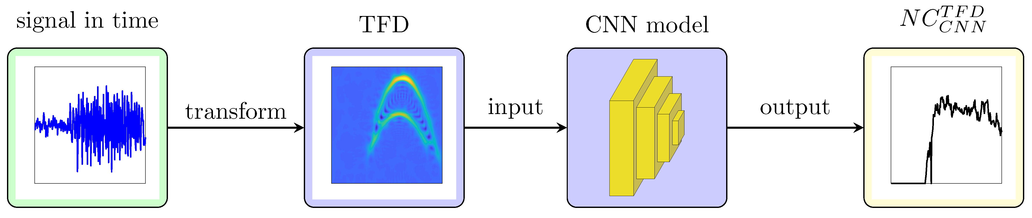
2.4. Summary of the Proposed Approach

The block diagram depicted in Figure 4 illustrates the fundamental steps of the proposed methodology. Initially, the signals provided by end-users are typically in the time domain. The first task is to transform these signals into their corresponding analytic representations, $z\left(t\right)$, particularly when dealing with real-valued signals. This transformation is achieved through the application of the Hilbert transform [7]. Subsequently, the TFD of the signal $z\left(t\right)$ needs to be computed, as detailed in Section 2.1. This computation involves selecting an appropriate TFD method from a set of options such as the WVD (given by (4)), the SPWV (given by (9)), the EMB (given by (11)), or the LOADTFD (given by (10)–(14)). The chosen TFD then serves as input to the proposed CNN corresponding to the selected TFD method. It is worth noting that from the three CNN models illustrated in Figure 2, the optimal model will be determined in the following section. Finally, the proposed CNN model produces a vector that represents the local number of components of the signal’s TFD. Depending on the application’s requirements, this vector may undergo rounding to the nearest integer value.

3. Results and Discussion

The performance evaluation of the CNN-based local component estimation method was conducted on four synthetic signals, each comprising $N_t=256$ samples. The first signal, labeled $z_{\mathrm{S}1}\left(t\right)$ and also used in prior works [19,39], consists of four LFM components with different amplitudes, expressed analytically as

$$\begin{array}{cc}\hfill z_{\mathrm{S}1}\left(t\right)& =\Pi \left(\frac{t-70}{40}\right)\left[e^{2j\pi \left(0.0037{(t-50)}^2\right)}+1.2e^{2j\pi \left(0.2(t-50)+0.0037{(t-50)}^2\right)}\right]+\hfill \\ \hfill & +\Pi \left(\frac{t-220}{40}\right)\left[e^{2j\pi \left(0.0037{(t-200)}^2\right)}+1.2e^{2j\pi \left(0.2(t-200)+0.0037{(t-200)}^2\right)}\right].\hfill \end{array}$$

(28)

The remaining three signals, designated as $z_{\mathrm{S}2}\left(t\right)$, $z_{\mathrm{S}3}\left(t\right)$, and $z_{\mathrm{S}4}\left(t\right)$, were randomly generated and include multiple components of both LFM and QFM components, each with distinct amplitudes. Their analytical forms are described as follows:

$$\begin{array}{cc}\hfill z_{\mathrm{S}2}\left(t\right)& =0.7384\Pi \left(\frac{t-177}{158}\right)e^{2j\pi \left(0.2249(t-98)+0.0034{(t-98)}^2-1.6407·{10}^{-5}{(t-98)}^3\right)}+\hfill \\ \hfill & +0.6433\Pi \left(\frac{t-154}{144}\right)e^{2j\pi \left(0.0891(t-82)+0.0027{(t-82)}^2-1.1826·{10}^{-5}{(t-82)}^3\right)},\hfill \end{array}$$

(29)

$$\begin{array}{cc}\hfill z_{\mathrm{S}3}\left(t\right)& =0.7631\Pi \left(\frac{t-232}{48}\right)e^{2j\pi \left(0.0307(t-208)+0.0066{(t-208)}^2-5.4592·{10}^{-5}{(t-208)}^3\right)}+\hfill \\ \hfill & +1.0279\Pi \left(\frac{t-127}{62}\right)e^{2j\pi \left(0.2618(t-96)+0.0083{(t-96)}^2-1.083·{10}^{-4}{(t-96)}^3\right)}+\hfill \\ \hfill & +0.9267\Pi \left(\frac{t-154}{204}\right)e^{2j\pi \left(0.3292(t-52)-0.0017{(t-52)}^2+3.7187·{10}^{-6}{(t-52)}^3\right)},\hfill \end{array}$$

(30)

$$\begin{array}{cc}\hfill z_{\mathrm{S}4}\left(t\right)& =0.897\Pi \left(\frac{t-129}{200}\right)e^{2j\pi \left(0.374(t-29)-8.985·{10}^{-4}{(t-29)}^2\right)}+\hfill \\ \hfill & +0.4057\Pi \left(\frac{t-200}{110}\right)e^{2j\pi \left(0.2447(t-145)+8.6464·{10}^{-4}{(t-145)}^2\right)}+\hfill \\ \hfill & +1.2129\Pi \left(\frac{t-195}{122}\right)e^{2j\pi \left(0.1804(t-134)+4.8770·{10}^{-4}{(t-134)}^2\right)}.\hfill \end{array}$$

(31)

Furthermore, signals $z_{\mathrm{S}2}\left(t\right),z_{\mathrm{S}3}\left(t\right)$ and $z_{\mathrm{S}4}\left(t\right)$ were embedded in AWGN with SNRs equal to 12, 16, and 9 dB, respectively. Real-world signals, namely gravitational (This research has made use of data, software, and/or web tools obtained from the LIGO Open Science Center (https://losc.ligo.org), a service of LIGO Laboratory and the LIGO Scientific Collaboration. LIGO is funded by the U.S. National Science Foundation.) ($z_{\mathrm{G}}\left(t\right)$) [1,11,39,47] and one representative of EEG seizure activity (the data and relevant code are publicly available at https://github.com/nabeelalikhan1/EEG-Classification-IF-and-GD-features (accessed on 14 May 2024)) ($z_{\mathrm{EEG}}\left(t\right)$) [11,14,22,33,34,48,49,50], were also employed for validation purposes. The preprocessing of the real-life signals involved established whitening and filtering techniques to enhance signal detection, as detailed in

Table 2. Summary of real-world dataset information.

Signal	Preprocessing Steps
gravitational, $z_{\mathrm{G}}\left(t\right)$	initially consisted of 3441 samples downsampled by a factor of 14, $N_t=256$ samples duration of $[0.25,0.45]$ s, frequency range of $[0,512]$ Hz
EEG, $z_{\mathrm{EEG}}\left(t\right)$	prefiltered using a 0.5 to 70 Hz analog bandpass filter downsampled to 256 Hz and further to 32 Hz, $N_t=256$ samples enhanced spike signatures using a differentiator filter [49,50,51,52]

. Notably, to ensure the integrity of the evaluation, none of the synthetic nor real-world signals were included in the training or validation datasets of the proposed CNN model. Note that the calculation of the LRE involved the following parameters: ${\alpha }_R=3$ and ${\Theta }_t=11$ as recommended in [11,16,24].

We utilized several metrics to assess the error between the obtained local number of components and the reference (or ideal) values. These metrics include the mean squared error (MSE), MAE, and maximum absolute error (MAX), defined as follows:

$$MSE={\displaystyle \frac{1}{N_t}}\sum _{t=1}^{N_t}{\left(N{C}_{CNN}^{\mathrm{Y}(t,f)}\left(t\right)-{\widehat{NC}}_t\left(t\right)\right)}^2,$$

(32)

$$MAE={\displaystyle \frac{1}{N_t}}\sum _{t=1}^{N_t}|N{C}_{CNN}^{\mathrm{Y}(t,f)}\left(t\right)-{\widehat{NC}}_t\left(t\right)|,$$

(33)

$$MAX=\underset{t=1,\cdots ,N_t}{\max }\left(|N{C}_{CNN}^{\mathrm{Y}(t,f)}\left(t\right)-{\widehat{NC}}_t\left(t\right)|\right).$$

(34)

Larger values of MSE, MAE, or MAX indicate greater disparities between the calculated and ideal local component counts, thus lower values are preferable.

To quantitatively evaluate the smoothness of the obtained $N{C}_t$ curve, we introduced a metric that considers successive changes from positive to negative. To begin with, we compute the differential vector, denoted as $\Delta \mathbf{NC}$, which tracks changes in $N{C}_t$ as follows:

$$\Delta \mathbf{NC}=[N{C}_t\left(2\right)-N{C}_t\left(1\right),N{C}_t\left(3\right)-N{C}_t\left(2\right),\dots ,N{C}_t\left(N_t\right)-N{C}_t(N_t-1)].$$

(35)

To discern alterations in the differential vector indicative of successive transitions from positive to negative, we are interested in instances where $\Delta \mathbf{NC}$ changes its sign from positive to negative. These transitions are identified by the set $PTN$, defined as

$$PTN=i\mid \Delta NC\left(i\right)>0\wedge \Delta NC(i+1)<0.$$

(36)

Subsequently, we compute the magnitudes of these transitions, $|\Delta N{C}_i|$, for each $i\in PTN$, and aggregate them to derive the total magnitude of changes, denoted as $TM$:

$$TM=\sum _{i\in PTN}|\Delta NC\left(i\right)|.$$

(37)

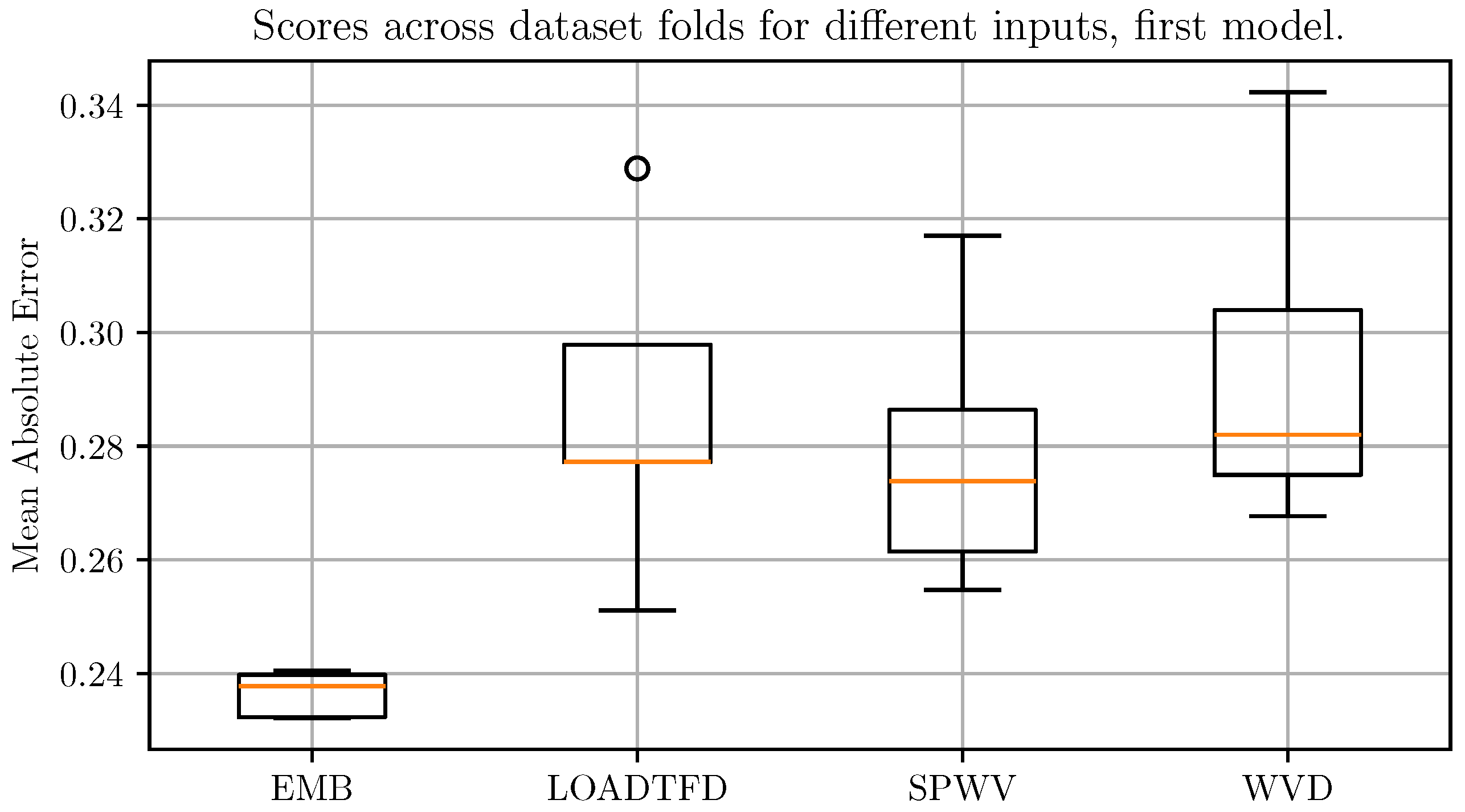
3.1. Model Evaluation

The training performance of the three developed networks can be seen below in

Table 3. Results of the three models trained on different input TFDs. Lower values indicate better performance. The best results per model are bolded.

Model	EMB		SPVW		WVD		LOADTFD
	$\overline{MAE}$	$\sigma$	$\overline{MAE}$	$\sigma$	$\overline{MAE}$	$\sigma$	$\overline{MAE}$	$\sigma$
1	0.23651	0.00361	0.27869	0.02202	0.29417	0.02963	0.28645	0.02588
2	0.17033	0.00215	0.18934	0.00192	0.23495	0.00293	0.18671	0.00526
3	0.22810	0.00559	0.22227	0.00522	0.26483	0.02865	0.22360	0.00600

. The results are given as the mean and standard deviation, denoted as $\sigma$, across different input methods.

For the first neural network, the best results are achieved using EMB as input, with an MAE of 0.24. The hyperparameters used were the batch size of 16, with the 10 training epochs. Actually, all models used the same number of epochs in the models that achieved 10 results, indicating that the created networks exhibit the overfitting issue relatively quickly. The comparison between the performance for different inputs is given in Figure 5. Clearly, the model based on the EMB shows the best performance on the test set, across all folds, with the slightest variation, performing better than even the best-performing folds of other models.

The second model shows the best results on EMB input, with an MAE of 0.17, using the batch size of 32. The comparison between the performance for different inputs is given in Figure 6. Again, EMB is shown to grant the best performance when used as the input to the model. Even the upper bound of the model error across folds with EMB is lower than the best-performing folds of the other models, as was the case in the previous example.

The third model achieves the best results, with an MAE of 0.22, using the batch size of 16 and 10 training epochs, on the SPWV input. Observing Figure 7, the scores between inputs are much more balanced, with only WVD showing a significantly higher error on the box plot. While EMB does show a remarkably low error of almost zero in the extreme case on a single fold, its median value is much closer to the remaining values.

The computational complexity of a CNN approach depends on the size of the CNN applied to the problem. When classifying a value with the CNN based on the size of the filters within the network. As such the smallest network used comprises 4,777,988 multiplication operations while the largest comprises 8,958,424. Still, since these are linear operations, the time complexity simplifies to $\mathcal{O}\left(n\right)$. Measuring the times necessary to infer the number of components based on the input is 0.35 ± 0.05 s for the smallest network, 0.38 ± 0.04 s for the medium-sized network and 0.42 ± 0.06 s for the largest network when using a i5 Intel(R) Core(TM) i5-9400 CPU @ 2.90 GHz to perform inference. It has to be noted that this time could be significantly lowered using a tensor or GPU-based machine for inference. Since the second model shows significantly better results compared to the other two models, it will be used for the further evaluation of different signals, the results of which will be presented in the continuation of this section.

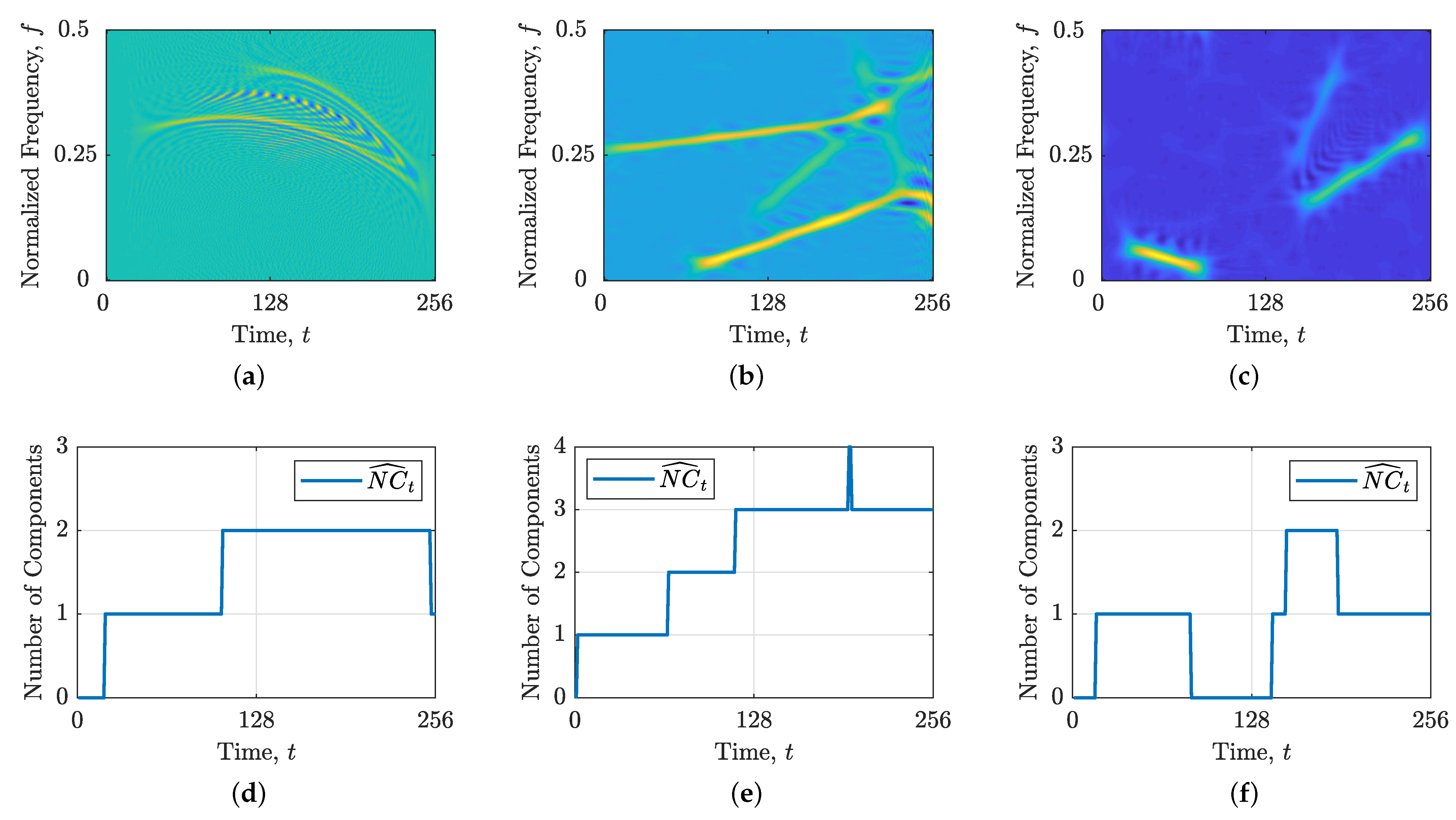
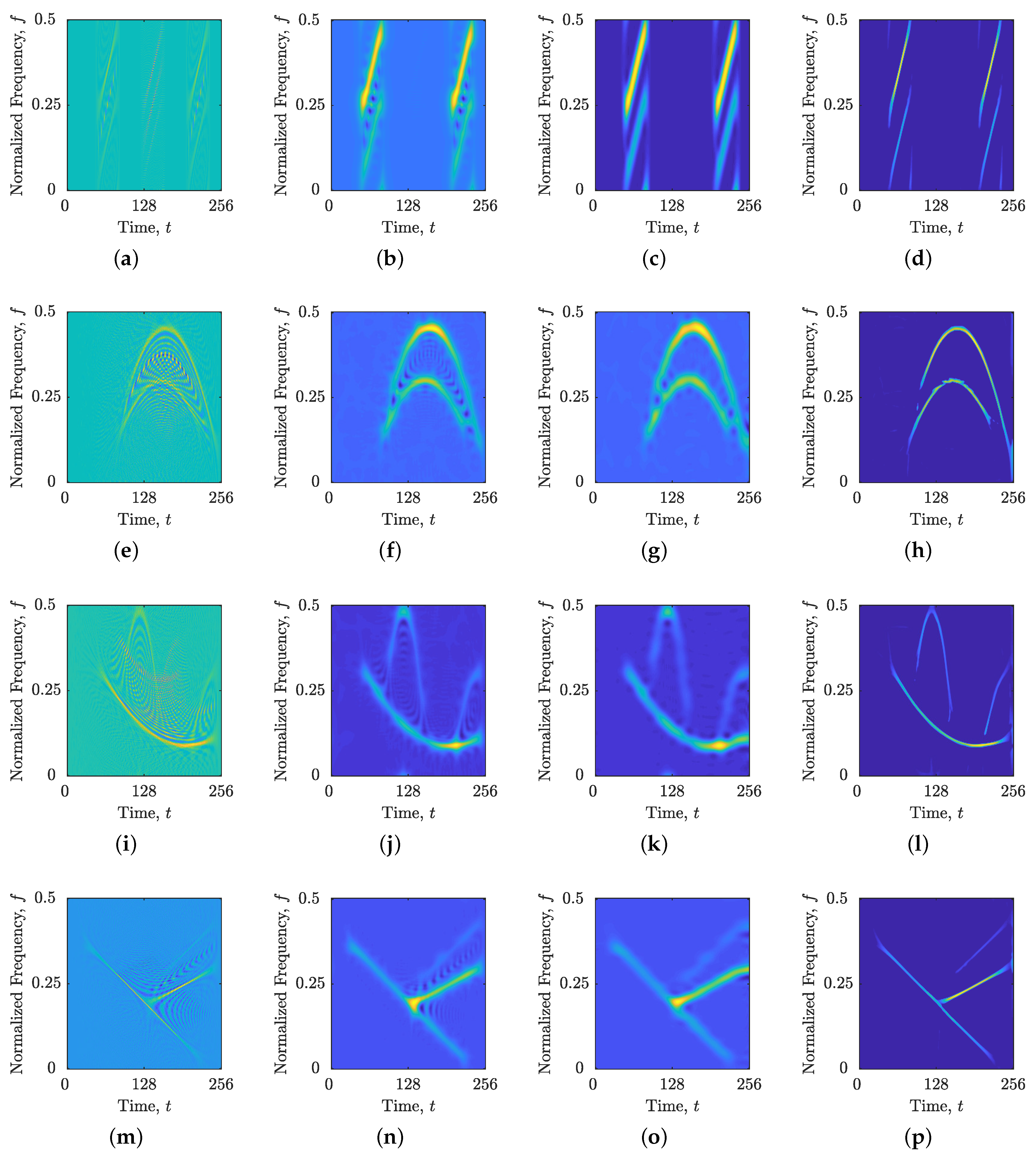
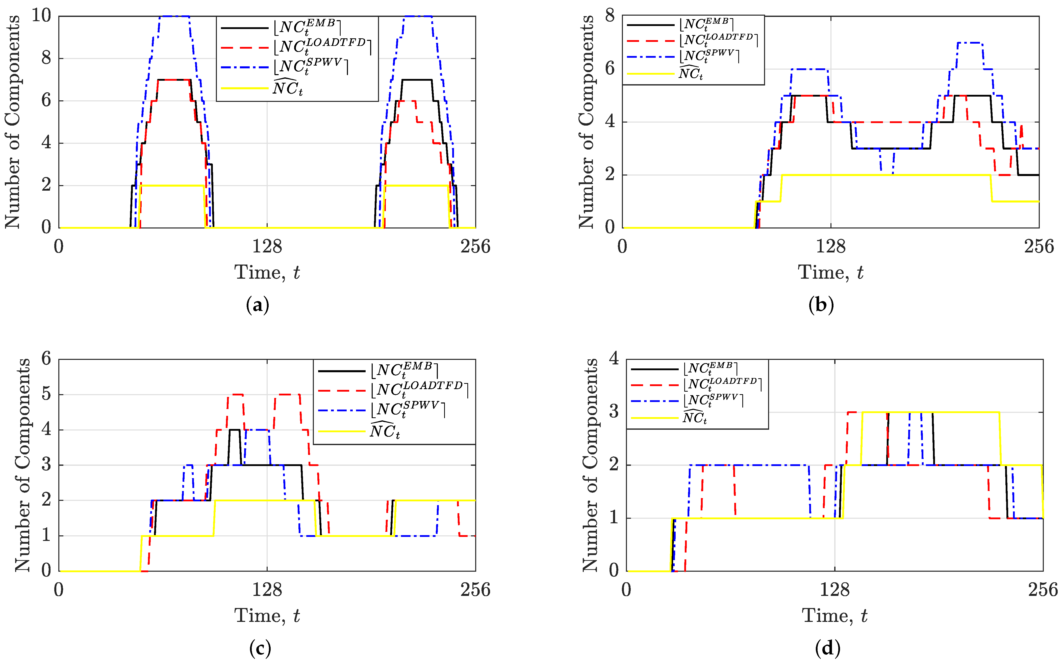
3.2. Results: Synthetic Signals

Figure 8 illustrates the WVDs, EMBs, SPWVs, and LOADTFDs of the considered synthetic signals $z_{\mathrm{S}1}\left(t\right)$, $z_{\mathrm{S}2}\left(t\right)$, $z_{\mathrm{S}3}\left(t\right)$, and $z_{\mathrm{S}4}\left(t\right)$. These TFDs served as inputs to the proposed CNN and represent multicomponent signals with closely spaced or intersecting components exhibiting randomized amplitudes.

The estimated local number of components (NCs) obtained using the LRE method with the EMB, SPWV, or LOADTFD as underlying TFDs is depicted in Figure 9. Across all three considered TFDs, the LRE method demonstrates notable limitations. Particularly, the NCs for components deviating from the time axis exhibit a pronounced artificial increase when compared to the ideal scenario, as consistently observed across all signal examples. Moreover, Figure 9c,d highlight that the LRE-based estimates diminish when components intersect, and the LRE method inadequately captures components of low amplitude.

Figure 10 and Figure 11 present the NCs obtained using the proposed CNN based on the EMB, SPWV, WVD, and LOADTFD. Visual inspection reveals that these CNN-based estimates mitigate the limitations of the LRE method and exhibit closer adherence to the ideal scenario. An exception is observed with the CNN-based estimated $N{C}_{CNN}$ on the WVD, which displays noticeable drops to zero throughout the entire time support of the signal components.

Table 4. Performance metrics of the proposed CNN-based versus LRE-based $\lfloor N{C}_t\rceil$ for the considered synthetic signals. The best results per metric are bolded.

Method	LRE			CNN
	EMB	SPWV	LOADTFD	WVD	EMB	SPWV	LOADTFD
$z_{S1}\left(t\right)$
$MSE$	6.0395	15.3992	4.2530	0.2332	0.1462	0.2569	0.1186
$MAE$	1.5880	2.4549	1.2017	0.1674	0.1502	0.2532	0.1288
$MAX$	5.0	8.0	5.0	2.0	2.0	2.0	1.0
$z_{S2}\left(t\right)$
$MSE$	2.9051	6.0316	3.2292	0.2964	0.0870	0.0830	0.0909
$MAE$	1.3433	1.8455	1.4592	0.2060	0.0730	0.0901	0.0987
$MAX$	3.0	5.0	3.0	2.0	1.0	1.0	1.0
$z_{S3}\left(t\right)$
$MSE$	0.4822	0.7628	1.7747	0.2055	0.0277	0.0435	0.0356
$MAE$	0.4464	0.6137	0.8927	0.1631	0.0300	0.0472	0.0343
$MAX$	2.0	2.0	3.0	2.0	1.0	1.0	1.0
$z_{S4}\left(t\right)$
$MSE$	0.3202	0.6917	0.6522	0.3834	0.1423	0.1265	0.1818
$MAE$	0.3047	0.7082	0.6052	0.2232	0.1502	0.1373	0.1545
$MAX$	1.0	1.0	2.0	3.0	1.0	1.0	1.0

presents the numerical results for the LRE and CNN-based NCs depicted in Figure 9, Figure 10 and Figure 11. These metrics complement observations from visual inspection and substantiate the superiority of the proposed CNN approach over the LRE method using any of the considered advanced TFDs: EMB, SPWV, or LOADTFD. In terms of MSE performance, an improvement compared to the original LRE method spans from 55.52% (EMB, $z_{S4}\left(t\right)$) to 98.63% (SPWV, $z_{S2}\left(t\right)$). In terms of MAE performance, the proposed CNN-based estimations achieve improvements spanning from 49.33% (EMB, $z_{S4}\left(t\right)$) to 96.16% (LOADTFD, $z_{S3}\left(t\right)$). MAX metric showed that CNN-based NCs using EMB, SPWV or LOADTFD have significantly lower maximum errors when compared to the LRE method’s NCs. Notably, the proposed CNN based on the WVD demonstrates inferior performance compared to other considered TFDs but still outperforms the LRE method, particularly evident for signals $z_{\mathrm{S}1}\left(t\right)$, $z_{\mathrm{S}2}\left(t\right)$, and $z_{\mathrm{S}3}\left(t\right)$.

In

Table 5. Total magnitude metric calculated from the local numbers of components obtained using the proposed CNN versus LRE method for the considered synthetic signals. The best results per signal are bolded.

Method	LRE			CNN
	EMB	SPWV	LOADTFD	WVD	EMB	SPWV	LOADTFD
$z_{S1}\left(t\right)$
$TM$	0.0087	0.0574	0.0804	11.5030	3.5436	5.1649	2.8838
$z_{S2}\left(t\right)$
$TM$	0.0165	0.0251	0.3095	12.6532	4.3124	3.6477	3.3645
$z_{S3}\left(t\right)$
$TM$	0.0406	0.0815	0.1659	21.1449	6.9535	5.2687	5.3525
$z_{S4}\left(t\right)$
$TM$	0.0263	0.0376	0.1002	27.4028	8.2332	8.3377	7.0315

, we present the analysis of the TM from consecutive positive to negative transitions of the raw NCs for the considered synthetic signals. Across all synthetic signal examples ($z_{\mathrm{S}1}\left(t\right)$, $z_{\mathrm{S}2}\left(t\right)$, $z_{\mathrm{S}3}\left(t\right)$, and $z_{\mathrm{S}4}\left(t\right)$), the TM for the LRE method yields lower values compared to the CNN approach. Specifically, the NCs obtained using the LRE method and the EMB consistently yield the lowest TM, while the NCs obtained using the CNN approach based on the WVD exhibits the highest volatility, thus highlighting it as the most fluctuant curve. Figure 1d presents the LRE-based raw curves, while Figure 10 and Figure 11 depict the CNN-based curves.

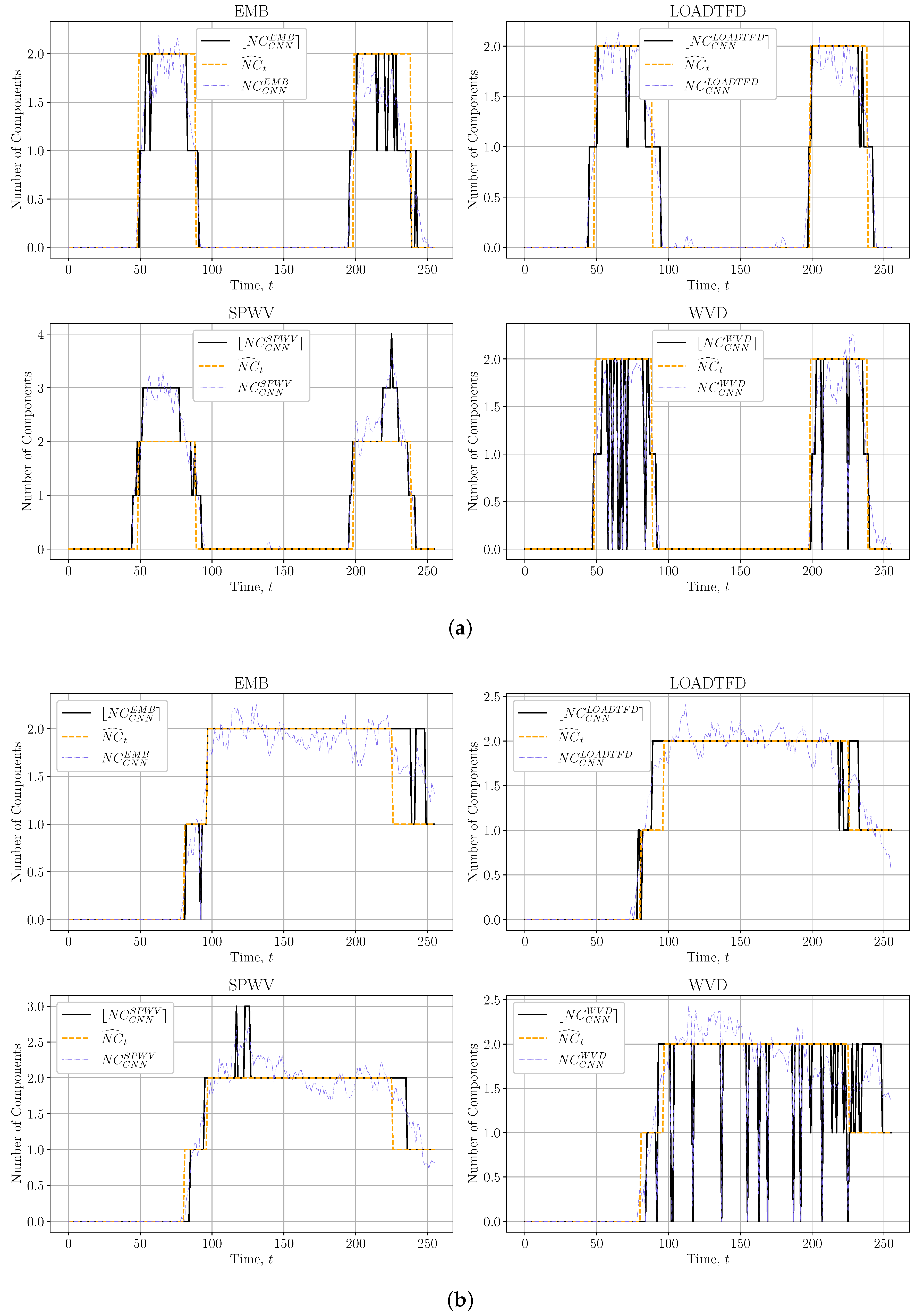
3.3. Results: Real-World Signals

Figure 12 presents the WVDs, EMBs, SPWVs, and LOADTFDs of the considered real-world signals $z_{\mathrm{EEG}}\left(t\right)$ and $z_{\mathrm{G}}\left(t\right)$. The TFDs of $z_{\mathrm{EEG}}\left(t\right)$ reveal the presence of a single tone component alongside several spikes, while those of $z_{\mathrm{G}}\left(t\right)$ exhibit a hyperbolic behavior in signal composition.

Notably, both spikes and segments of hyperbolic FM components deviate from the time axis, rendering them unsuitable for analysis using the original LRE method, as evident in Figure 13. Specifically, spikes introduce significant errors in the estimated local number of components (NCs), causing an increase even up to seven for the SPWV example. A similar phenomenon is observed for segments of the gravitational signal component, where the expected value of NCs should remain constant at one throughout the signal’s duration.

Figure 14 portrays the local numbers of components of $z_{\mathrm{EEG}}\left(t\right)$ and $z_{\mathrm{G}}\left(t\right)$ obtained using the proposed CNN. Upon visual inspection, these results demonstrate improvements over the local number of components estimated using the LRE method, reinforcing observations made for synthetic signals. For $z_{\mathrm{EEG}}\left(t\right)$, the CNN-based NCs, particularly when utilizing the LOADTFD and EMB, accurately identify spikes and indicate the presence of two components during spike occurrences. Furthermore, the NCs based on the LOADTFD notably preserve the tone component. Regarding $z_{\mathrm{G}}\left(t\right)$, the CNN-based NCs derived from the LOADTFD, EMB, and SPWV exhibit reduced errors compared to those resulting from the LRE method. These CNN-based estimates consistently indicate the presence of a single component for the majority of time instances. However, it is noteworthy that the NCs obtained using the CNN based on the WVD consistently demonstrate drops to zero, indicating a limitation in capturing components using this particular method.

Noise Sensitivity Analysis

To assess the impact of noise on the estimated local number of components (NCs) using the proposed CNN, a comprehensive comparative analysis is conducted using MSE values in decibels (dB). These values are calculated between the estimated NCs for noise-free and noisy synthetic signals. The signals are deliberately embedded in AWGN across four SNR levels ranging from 9 dB down to 0 dB. It is essential to note that the reported results are based on 1000 independent noise realizations. The findings, as presented in

Table 6. MSE in dB between the estimated local numbers of components for noise-free and noisy synthetic signals embedded in AWGN with SNR $=\{0,3,6,9\}$. Values are averaged from 1000 simulations of the signals with different noise realizations.

SNR	LRE			CNN
	EMB	SPWV	LOADTFD	WVD	EMB	SPWV	LOADTFD
$z_{S1}\left(t\right)$
0 dB	7.0717	8.9815	1.2492	−7.3362	−10.1252	−2.5303	−3.4793
3 dB	−0.0602	1.2639	−2.5805	−9.1106	−13.2208	−4.3948	−7.9652
6 dB	−4.3212	−2.3822	−4.7755	−10.8443	−15.5875	−8.0980	−11.3878
9 dB	−7.4027	−4.6578	−6.0891	−13.0621	−16.8464	−11.1452	−13.6729
$z_{S2}\left(t\right)$
0 dB	6.1719	7.1244	2.9371	−6.8008	−2.2093	−2.8176	−0.6299
3 dB	−2.3075	−0.8763	−1.9152	−7.9310	−6.2736	−6.2562	−4.5125
6 dB	−8.2379	−5.0221	−5.4218	−9.2890	−9.7337	−8.9689	−7.4425
9 dB	−10.3168	−7.5535	−7.7290	−10.4291	−12.3286	−10.7149	−11.0231
$z_{S3}\left(t\right)$
0 dB	3.5811	4.5762	0.1177	−6.9751	−4.1474	−3.8873	−3.8927
3 dB	−2.8621	−0.9289	−2.3439	−9.2096	−7.2424	−6.3909	−7.0320
6 dB	−6.5891	−4.9981	−5.0144	−11.2254	−10.2509	−8.8513	−9.9522
9 dB	−8.6492	−7.6334	−7.6453	−13.8818	−13.1040	−10.5345	−12.6545
$z_{S4}\left(t\right)$
0 dB	2.1689	2.3456	−1.4015	−5.0527	−3.3821	−2.8123	−3.2841
3 dB	−3.9897	−3.4443	−5.2725	−7.1899	−4.7324	−4.1367	−5.1539
6 dB	−6.9598	−5.1053	−7.3501	−10.0241	−7.5194	−6.8762	−8.2932
9 dB	−9.7742	−6.5977	−9.5550	−12.8951	−9.8615	−9.2832	−10.7190

, demonstrate the superiority of the proposed CNN over the LRE method across all synthetic signal examples and SNR levels. This conclusion is substantiated by the CNN consistently achieving lower MSE values, indicating enhanced accuracy in estimating the local number of components amidst varying levels of noise interference.

3.4. Interpretation of the Results

As is evident from Figure 9, Figure 10 and Figure 11, as well as supported by the numerical results in Table 4, the CNN-based estimations of local component numbers surpass those obtained through the LRE method for all synthetic signal examples, which were unseen by the CNN during training. Additionally, EMB, SPWV, and LOADTFD emerged as competitive choices for TFDs in CNN training.

The findings and conclusions drawn from the synthetic signals also extend to real-world EEG seizure and gravitational signals, as depicted in Figure 13 and Figure 14. Our research aimed to demonstrate that utilizing a diverse training set not specifically tailored to the application can enhance estimation results for real-world signals showcasing LFM and QFM components.

Table 6 illustrates that CNN-based estimates exhibit significantly lower sensitivity to AWGN across considered SNR levels compared to the LRE method. While superior smoothing capabilities of the LOADTFD benefit LRE at lower SNRs, the proposed CNN, particularly when using EMB, LOADTFD, and SPWV, demonstrates competitive performance across all SNR levels. Notably, CNN’s performance with WVD input surpasses that of other TFDs for most considered signals, attributed to training with interference-corrupted TFD such as WVD, rendering noise inclusion less apparent compared to other TFDs.

An added advantage of implementing the proposed CNN methodology is the circumvention of the necessity for additional parameter tuning, for example in the LRE method. Furthermore, users are liberated from the responsibility of identifying and separating components deemed more suitable for localization via frequency slices, as typically entailed in the NBRE version of the LRE method.

The enhancement in estimated local component numbers holds the potential to improve the performance of numerous LRE-based applications. For instance, more precise estimation of local component numbers could notably refine IF estimation techniques employed in algorithms such as those detailed in [6,53]. Additionally, the iterative thresholding algorithm for sparse TFD reconstruction proposed in [19], currently relying on a balance between outputs from STRE or NBRE depending on their correctness for a given signal, could potentially undergo computational simplification by exclusively utilizing the proposed CNN-based estimate.

Limitations of the Proposed Approach

Similar to the LRE method, the results showed that the CNN’s performance is affected by the clarity of its underlying TFD. Given the computational simplicity of the WVD over other QTFDs, requiring only the WVD from a user would be preferable. However, the CNN based on the WVD exhibited volatility and notable estimation drops, thus indicating lower performance. Consequently, it is advisable to use the CNN based on EMB, SPWV, or LOADTFD instead.

The results presented in Table 5 suggest that unrounded curves representing local component numbers exhibit smoother transitions with the LRE method compared to the proposed CNN. This smoother behavior in LRE can be attributed to its use of sliding windows, where the window size influences the curve’s smoothness and dynamics. While larger window sizes result in smoother curves, they may compromise prompt component detection. Conversely, smaller window sizes may emphasize unresolved cross-terms or noise samples, leading to reduced accuracy in estimated numbers and poorer curve smoothness [24]. Although local component numbers are typically rounded for practical applications [18,19,20,21,39,54], raw output from the proposed CNN may limit its usage in cases where the identification of local maxima is required. Therefore, our future research will explore refining the CNN’s raw output through careful analysis of smoothing filters and methods while preserving its dynamic capabilities. It is anticipated that smoothed curves will reduce inaccurate spikes that may appear in CNN-based estimates when rounding to the nearest integer.

Observing the CNN part of the study, it has to be noted that a more detailed exploration of the possible hyperparameter influences—such as model shapes or training epochs—could always be performed. Still, due to the presented architectures having achieved satisfying scores, we deemed a more precise exploration unnecessary.

While this study aimed to propose a versatile approach applicable to diverse signal examples, it is recognized that certain applications may benefit from constructing training datasets tailored to signals exhibiting specific characteristics within specific noise environments. This may entail the integration of large datasets comprising real-world signals specific to an application, either as a supplement or substitute for synthetic datasets. The observed enhancements in our approach, which is not tailored to any specific application, underscore the potential utility of developing application-specific datasets. Such datasets are anticipated to further enhance estimation performance in targeted applications by aligning more closely with the characteristics and challenges present in those contexts.

4. Conclusions

Our study presents evidence supporting the superiority of CNN over the traditional LRE method for estimating local numbers of components in signal processing tasks. Through extensive analysis across diverse synthetic and real-world signal examples, CNN-based estimations consistently outperform LRE, underscoring the robustness and generalization capability of the CNN approach. We observed that among the TFDs utilized for CNN training, including EMB, SPWV, and LOADTFD, each emerged as a competitive option. Despite the smoother transitions seen with LRE, CNN offers dynamic capabilities and a higher resilience to noise, making it well-suited for applications in noisy environments.

Our findings also extend to real-world signals, such as EEG seizure and gravitational signals, where CNN-based estimations showcase promising results even without specific training for these signals. This highlights the adaptability and effectiveness of CNNs in practical scenarios.

In conclusion, our study provides strong support for the efficacy and versatility of CNNs in signal processing applications. These findings suggest opportunities for the further refinement of CNN models, the exploration of additional training datasets tailored to specific applications, and the investigation of advanced smoothing techniques to enhance accuracy and reliability in real-world scenarios.

References

1. Lopac, N. Detection of Gravitational-Wave Signals from Time-Frequency Distributions Using Deep Learning. Ph.D. Thesis, University of Rijeka, Faculty of Engineering, Rijeka, Croatia, 2022. [Google Scholar]
2. Milczarek, H.; Leśnik, C.; Djurović, I.; Kawalec, A. Estimating the Instantaneous Frequency of Linear and Nonlinear Frequency Modulated Radar Signals—A Comparative Study. Sensors 2021, 21, 2840. [Google Scholar] [CrossRef] [PubMed]
3. Swiercz, E.; Janczak, D.; Konopko, K. Detection of LFM Radar Signals and Chirp Rate Estimation Based on Time-Frequency Rate Distribution. Sensors 2021, 21, 5415. [Google Scholar] [CrossRef]
4. Dózsa, T.; Jurdana, V.; Šegota, S.B.; Volk, J.; Radó, J.; Soumelidis, A.; Kovács, P. Road Type Classification Using Time-Frequency Representations of Tire Sensor Signals. IEEE Access 2024, 12, 53361–53372. [Google Scholar] [CrossRef]
5. Lerga, J.; Saulig, N.; Lerga, R.; Štajduhar, I. TFD thresholding in estimating the number of EEG components and the dominant if using the short-term Rényi entropy. In Proceedings of the 10th International Symposium on Image and Signal Processing and Analysis, Ljubljana, Slovenia, 18–20 September 2017; pp. 80–85. [Google Scholar]
6. Lerga, J.; Saulig, N.; Stanković, L.; Seršić, D. Rule-based EEG classifier utilizing local entropy of time–frequency distributions. Mathematics 2021, 9, 451. [Google Scholar] [CrossRef]
7. Boashash, B. Time-Frequency Signal Analysis and Processing, A Comprehensive Reference, 2nd ed.; EURASIP and Academic Press Series in Signal and Image Processing; Elsevier: London, UK, 2016. [Google Scholar]
8. Stankovic, L.; Dakovic, M.; Thayaparan, T. Time-Frequency Signal Analysis with Applications; Artech House Publishers: Boston, MA, USA, 2013. [Google Scholar]
9. Pachori, R.B. Time-Frequency Analysis Techniques and Their Applications; CRC Press: Boca Raton, FL, USA, 2023. [Google Scholar]
10. Akan, A.; Karabiber Cura, O. Time–frequency signal processing: Today and future. Digit. Signal Process. 2021, 119, 103216. [Google Scholar] [CrossRef]
11. Jurdana, V. A Multi-Objective Optimization Procedure for Locally Adaptive Time-Frequency Analysis with Application in EEG Signal Processing. Ph.D. Thesis, University of Rijeka, Faculty of Engineering, Rijeka, Croatia, 2023. [Google Scholar]
12. Lerga, J.; Sucic, V.; Boashash, B. An efficient algorithm for instantaneous frequency estimation of nonstationary multicomponent signals in low SNR. EURASIP J. Adv. Signal Process. 2011, 2011, 725189. [Google Scholar] [CrossRef]
13. Khan, N.A.; Mohammadi, M.; Djurović, I. A modified viterbi algorithm-based IF estimation algorithm for adaptive directional time-frequency distributions. Circuits Syst. Signal Process. 2019, 38, 2227–2244. [Google Scholar] [CrossRef]
14. Khan, N.A.; Ali, S. Classification of EEG signals using adaptive time-frequency distributions. Metrol. Meas. Syst. 2016, 23, 251–260. [Google Scholar] [CrossRef]
15. Sucic, V.; Saulig, N.; Boashash, B. Estimating the number of components of a multicomponent nonstationary signal using the short-term time-frequency Rényi entropy. EURASIP J. Adv. Signal Process. 2011, 2011, 125. [Google Scholar] [CrossRef]
16. Sucic, V.; Saulig, N.; Boashash, B. Analysis of local time-frequency entropy features for nonstationary signal components time supports detection. Digit. Signal Process. 2014, 34, 56–66. [Google Scholar] [CrossRef]
17. Saulig, N.; Orović, I.; Sucic, V. Optimization of quadratic time–frequency distributions using the local Rényi entropy information. Signal Process. 2016, 129, 17–24. [Google Scholar] [CrossRef]
18. Jurdana, V.; Volaric, I.; Sucic, V. The local Rényi entropy based shrinkage algorithm for sparse TFD reconstruction. In Proceedings of the 2020 International Conference on Broadband Communications for Next Generation Networks and Multimedia Applications (CoBCom), Graz, Austria, 7–9 July 2020; pp. 1–8. [Google Scholar] [CrossRef]
19. Jurdana, V.; Volaric, I.; Sucic, V. Sparse time-frequency distribution reconstruction based on the 2D Rényi entropy shrinkage algorithm. Digit. Signal Process. 2021, 118, 103225. [Google Scholar] [CrossRef]
20. Jurdana, V.; Volaric, I.; Sucic, V. A sparse TFD reconstruction approach using the S-method and local entropies information. In Proceedings of the 2021 12th International Symposium on Image and Signal Processing and Analysis (ISPA), Zagreb, Croatia, 13–15 September 2021; pp. 4–9. [Google Scholar] [CrossRef]
21. Jurdana, V.; Volaric, I.; Sucic, V. Application of the 2D local entropy information in sparse TFD reconstruction. In Proceedings of the 2022 International Conference on Broadband Communications for Next Generation Networks and Multimedia Applications (CoBCom), Graz, Austria, 12–14 July 2022; pp. 1–7. [Google Scholar] [CrossRef]
22. Jurdana, V.; Vrankic, M.; Lopac, N.; Jadav, G.M. Method for automatic estimation of instantaneous frequency and group delay in time-frequency distributions with application in EEG seizure signals analysis. Sensors 2023, 23, 4680. [Google Scholar] [CrossRef] [PubMed]
23. Jurdana, V. Local Rényi entropy-based Gini index for measuring and optimizing sparse time-frequency distributions. Digit. Signal Process. 2024, 147, 104401. [Google Scholar] [CrossRef]
24. Saulig, N.; Lerga, J.; Miličić, S.; Tomasović, Z. Block-adaptive Rényi entropy-based denoising for non-stationary signals. Sensors 2022, 22, 8251. [Google Scholar] [CrossRef]
25. Saulig, N.; Lerga, J.; Milanović, Z.; Ioana, C. Extraction of useful information content from noisy signals based on structural affinity of clustered TFDs’ coefficients. IEEE Trans. Signal Process. 2019, 67, 3154–3167. [Google Scholar] [CrossRef]
26. Bruni, V.; Tartaglione, M.; Vitulano, D. A Signal Complexity-Based Approach for AM–FM Signal Modes Counting. Mathematics 2020, 8, 2170. [Google Scholar] [CrossRef]
27. Saulig, N.; Pustelnik, N.; Borgnat, P.; Flandrin, P.; Sucic, V. Instantaneous counting of components in nonstationary signals. In Proceedings of the 21st European Signal Processing Conference (EUSIPCO 2013), Marrakech, Morocco, 9–13 September 2013; pp. 1–5. [Google Scholar]
28. Shang, L.; Zhang, Z.; Tang, F.; Cao, Q.; Pan, H.; Lin, Z. CNN-LSTM hybrid model to promote signal processing of ultrasonic guided lamb waves for damage detection in metallic pipelines. Sensors 2023, 23, 7059. [Google Scholar] [CrossRef]
29. Zaman, W.; Ahmad, Z.; Siddique, M.F.; Ullah, N.; Kim, J.M. Centrifugal Pump Fault Diagnosis Based on a Novel SobelEdge Scalogram and CNN. Sensors 2023, 23, 5255. [Google Scholar] [CrossRef]
30. Patil, S.S.; Pardeshi, S.S.; Patange, A.D. Health Monitoring of Milling Tool Inserts Using CNN Architectures Trained by Vibration Spectrograms. CMES-Comput. Model. Eng. Sci. 2023, 136, 177–199. [Google Scholar] [CrossRef]
31. Jung, H.; Choi, S.; Lee, B. Rotor fault diagnosis method using CNN-Based transfer learning with 2D sound spectrogram analysis. Electronics 2023, 12, 480. [Google Scholar] [CrossRef]
32. Khan, N.A.; Boashash, B. Multi-component instantaneous frequency estimation using locally adaptive directional time frequency distributions. Int. J. Adapt. Control. Signal Process. 2016, 30, 429–442. [Google Scholar] [CrossRef]
33. Mohammadi, M.; Pouyan, A.A.; Khan, N.A.; Abolghasemi, V. Locally Optimized Adaptive Directional Time-Frequency Distributions. Circuits Syst. Signal Process. 2018, 37, 3154–3174. [Google Scholar] [CrossRef]
34. Mohammadi, M.; Ali Khan, N.; Hassanpour, H.; Hussien Mohammed, A. Spike Detection Based on the Adaptive Time-Frequency Analysis. Circuits Syst. Signal Process. 2020, 39, 5656–5680. [Google Scholar] [CrossRef]
35. Stanković, L. A measure of some time–frequency distributions concentration. Signal Process. 2001, 81, 621–631. [Google Scholar] [CrossRef]
36. Baraniuk, R.G.; Flandrin, P.; Janssen, A.J.E.M.; Michel, O.J.J. Measuring time-frequency information content using the Rényi entropies. IEEE Trans. Inf. Theory 2001, 47, 1391–1409. [Google Scholar] [CrossRef]
37. Aviyente, S.; Williams, W.J. Minimum entropy time-frequency distributions. IEEE Signal Process. Lett. 2005, 12, 37–40. [Google Scholar] [CrossRef]
38. Principe, J. Information Theoretic Learning: Renyi’s Entropy and Kernel Perspectives; Springer: New York, NY, USA, 2010. [Google Scholar] [CrossRef]
39. Jurdana, V.; Lopac, N.; Vrankic, M. Sparse Time-Frequency Distribution Reconstruction Using the Adaptive Compressed Sensed Area Optimized with the Multi-Objective Approach. Sensors 2023, 23, 4148. [Google Scholar] [CrossRef] [PubMed]
40. Taye, M.M. Theoretical understanding of convolutional neural network: Concepts, architectures, applications, future directions. Computation 2023, 11, 52. [Google Scholar] [CrossRef]
41. Bartlett, P.L.; Montanari, A.; Rakhlin, A. Deep Learning: A Statistical Viewpoint; Cambridge University Press: Cambridge, UK, 2021; Volume 30, pp. 87–201. [Google Scholar]
42. Boashash, B.; Khan, N.A.; Ben-Jabeur, T. Time–frequency features for pattern recognition using high-resolution TFDs: A tutorial review. Digit. Signal Process. 2015, 40, 1–30. [Google Scholar] [CrossRef]
43. Ai, D.; Cheng, J. A deep learning approach for electromechanical impedance based concrete structural damage quantification using two-dimensional convolutional neural network. Mech. Syst. Signal Process. 2023, 183, 109634. [Google Scholar] [CrossRef]
44. Kumar, A.; Singh, K.P.; Kumar, S.; Vetrivendan, L. Image classification in python using Keras. In Proceedings of the Data Analytics and Management: ICDAM 2021; Springer: Berlin/Heidelberg, Germany, 2022; Volume 1, pp. 541–556. [Google Scholar]
45. Singh, R.; Agarwal, B.B. An automated brain tumor classification in MR images using an enhanced convolutional neural network. Int. J. Inf. Technol. 2023, 15, 665–674. [Google Scholar] [CrossRef]
46. Boashash, B.; Jawad, B.K.; Ouelha, S. Refining the ambiguity domain characteristics of non-stationary signals for improved time–frequency analysis: Test case of multidirectional and multicomponent piecewise LFM and HFM signals. Digit. Signal Process. 2018, 83, 367–382. [Google Scholar] [CrossRef]
47. Lopac, N.; Hržić, F.; Vuksanović, I.P.; Lerga, J. Detection of non-stationary GW signals in high noise from Cohen’s class of time-frequency representations using deep learning. IEEE Access 2021, 10, 2408–2428. [Google Scholar] [CrossRef]
48. Boashash, B.; Azemi, G.; Ali Khan, N. Principles of time–frequency feature extraction for change detection in non-stationary signals: Applications to newborn EEG abnormality detection. Pattern Recognit. 2015, 48, 616–627. [Google Scholar] [CrossRef]
49. Khan, N.A.; Ali, S.; Choi, K. An instantaneous frequency and group delay based feature for classifying EEG signals. Biomed. Signal Process. Control. 2021, 67, 102562. [Google Scholar] [CrossRef]
50. Khan, N.A.; Ali, S. A new feature for the classification of non-stationary signals based on the direction of signal energy in the time–frequency domain. Comput. Biol. Med. 2018, 100, 10–16. [Google Scholar] [CrossRef]
51. Majumdar, K. Differential operator in seizure detection. Comput. Biol. Med. 2012, 42, 70–74. [Google Scholar] [CrossRef]
52. Stevenson, N.; O’Toole, J.; Rankine, L.; Boylan, G.; Boashash, B. A nonparametric feature for neonatal EEG seizure detection based on a representation of pseudo-periodicity. Med. Eng. Phys. 2012, 34, 437–446. [Google Scholar] [CrossRef]
53. Rankine, L.; Mesbah, M.; Boashash, B. IF estimation for multicomponent signals using image processing techniques in the time–frequency domain. Signal Process. 2007, 87, 1234–1250. [Google Scholar] [CrossRef]
54. Volaric, I.; Sucic, V.; Stankovic, S. A Data Driven Compressive Sensing Approach for Time-Frequency Signal Enhancement. Signal Process. 2017, 141, 229–239. [Google Scholar] [CrossRef]
Figure 1. (a) LOADTFD of a signal with two distinct components; (b) LOADTFD of a signal with two components intersected at t = 128 ; (c) LOADTFD of a signal with three components with different amplitudes embedded in AWGN with SNR = 2 dB; (d) N C ^ t , N C t and N C t corresponding to the LOADTFD in (a); (e) N C ^ t , N C t and N C t corresponding to the LOADTFD in (b); (f) N C ^ t , N C t i t e r and N C t corresponding to the LOADTFD in (c). N C t and N C t were obtained using the original LRE method in [15], while N C t i t e r was obatined using the iterative LRE method in [27].
Mathematics 12 01661 g001
Figure 2. The three proposed CNN models: (a) model 1, (b) model 2, (c) model 3.
Mathematics 12 01661 g002
Figure 3. For three random signal examples of the CNN training set: (a) WVD; (b) SPWV; (c) EMB; (d) N C ^ t corresponding to the WVD in (a); (e) N C ^ t corresponding to the SPWV in (b); (f) N C ^ t corresponding to the WVD in (c). TFDs in (ac) represent inputs to the CNN, while N C ^ t in (df) represent desired outputs.
Mathematics 12 01661 g003
Figure 4. Block diagram of the proposed approach.
Mathematics 12 01661 g004
Figure 5. The performance of the first model for different input TFDs. Lower values indicate better performance.
Mathematics 12 01661 g005
Figure 6. The performance of the second model for different input TFDs. Lower values indicate better performance.
Mathematics 12 01661 g006
Figure 7. The performance of the third model for different input TFDs. Lower values indicate better performance.
Mathematics 12 01661 g007
Figure 8. For the considered synthetic signals: (a) WVD of z S 1 ( t ) ; (b) EMB of z S 1 ( t ) ; (c) SPWV of z S 1 ( t ) ; (d) LOADTFD of z S 1 ( t ) ; (e) WVD of z S 2 ( t ) ; (f) EMB of z S 2 ( t ) ; (g) SPWV of z S 2 ( t ) ; (h) LOADTFD of z S 2 ( t ) ; (i) WVD of z S 3 ( t ) ; (j) EMB of z S 3 ( t ) ; (k) SPWV of z S 3 ( t ) ; (l) LOADTFD of z S 3 ( t ) ; (m) WVD of z S 4 ( t ) ; (n) EMB of z S 4 ( t ) ; (o) SPWV of z S 4 ( t ) ; and (p) LOADTFD of z S 4 ( t ) .
Mathematics 12 01661 g008
Figure 9. Local numbers of component obtained using the LRE method and different TFDs versus the ideal N C ^ t (yellow line) for the considered synthetic signals: (a) z S 1 ( t ) ; (b) z S 2 ( t ) ; (c) z S 3 ( t ) ; and (d) z S 4 ( t ) .
Mathematics 12 01661 g009
Figure 10. Local numbers of component obtained using the proposed CNN and different TFDs versus the ideal N C ^ t for the considered synthetic signals: (a) z S 1 ( t ) ; and (b) z S 2 ( t ) .
Mathematics 12 01661 g010
Figure 11. Local numbers of component obtained using the proposed CNN and different TFDs versus the ideal N C ^ t for the considered synthetic signals: (a) z S 3 ( t ) ; and (b) z S 4 ( t ) .
Mathematics 12 01661 g011
Figure 12. For the considered real-world signals: (a) WVD of z EEG ( t ) ; (b) EMB of z EEG ( t ) ; (c) SPWV of z EEG ( t ) ; (d) LOADTFD of z EEG ( t ) ; (e) WVD of z G ( t ) ; (f) EMB of z G ( t ) ; (g) SPWV of z G ( t ) ; and (h) LOADTFD of z G ( t ) .
Mathematics 12 01661 g012
Figure 13. Local numbers of component obtained using the LRE method and different TFDs for the considered real-world signals: (a) z EEG ( t ) ; and (b) z G ( t ) .
Mathematics 12 01661 g013
Figure 14. Local numbers of component obtained using the proposed CNN and different TFDs versus the ideal N C ^ t for the considered real-world signals: (a) z EEG ( t ) ; and (b) z G ( t ) .
Mathematics 12 01661 g014