Mathematical Logic Model for Analysing the Controllability of Mining Equipment

Abstract

The issues of the evaluation and prediction of the reliability and testability of mining machinery and equipment are becoming particularly relevant, since the safety of technological processes and human life is reaching a new level of realisation due to changes in mining technology. The work is devoted to the development of a logical model for analysing the controllability of mining equipment. The paper presents a model of reliability of the operation of mining equipment on the example of a mine load and passenger hoist. This generalised model is made in the form of a graph of transitions and supplemented with a system of equations. The model allows for the estimation of the reliability of equipment elements and equipment as a whole. A mathematical and logical model for the calculation of the availability and downtime coefficients of various designs of mining equipment systems is proposed. This model became the basis for the methods to calculate the optimal values of diagnostic depth. At these calculated values, the maximum value of availability factor will be obtained. In this paper, an analytical study was carried out and dependences of the readiness factor of parameters of the investigated system such as the intensity of control of technical systems, intensity of failures, etc., were constructed. The paper proposes a mathematical model to assess the reliability of mine hoisting plants through its integration into the method of improving the reliability of mine hoisting plants.

1. Introduction

As the depth of mineralisation increases with an increasing depth of mineralisation and the productivity of lifting systems under conditions of unstable loads, the requirements of quality parameters of elements of the lifting complex elements as well as their reliability and durability are increasing [1,2,3].

The significant depth of a shaft, the enlargement of mining enterprises, and an increase in the number of operating horizons significantly complicate the functioning process of mine hoisting installations. This causes an increase in loads on mine hoisting installations and the intensity of their work, which leads to an increase in the number of electrical failures and accelerated wear of the mechanical parts of mine hoisting plants [4,5].

Therefore, issues of improving the reliability of mine hoisting plants are extremely urgent. At the same time, the challenges of increasing the reliability and continuity in the operation of mine hoisting installations to ensure safety, regulated by rules and regulations must be met. Of great importance is the problem is defining the work reliability of mine hoisting installations and the development of effective ways to improve the operational reliability of the hoisting plant as mine hoisting plants are characterised by a high degree of complexity [6,7].

Simultaneously, the increasing complexity increases the responsibility functions performed by it. The provision of fail-safe operation of the plant is impossible without automating the procedures of technical diagnostics, function checks, and fault finding. Mine hoisting plants belong to the class of recoverable systems, and their reliability can be improved by reducing the time spent on the search and elimination of a defect. This issue cannot be solved without the appropriate adaptation of these systems to the technical diagnostics [8,9].

The increase in the number of mine workings and the growth in mineral extraction is now accompanied by an increase in the productivity of the equipment used. One of the most important elements of the mining industry is hoisting equipment. Under conditions of mining growth, these units also work under increasing loads. At the same time, the requirements for the quality parameters of such lifting units are increasing. In order to increase the production level and sustainable functioning of the whole mining system, it is necessary to increase the reliability and durability of hoisting plants [3]. However, an increase in the shaft depth, the growth of the scale of mining enterprises, and increase in the number of operating horizons significantly complicate the functioning of mine hoisting plants [5]. This leads to an increased load on them as well as an increase in their workload, which entails more frequent failures of electrical equipment and the faster wear of the mechanical components of mine hoisting plants [7]. In these conditions, it is extremely important to find ways to improve the reliability of mine hoisting plants. An improvement in reliability can be achieved through a comprehensive approach. This approach will include the improvement of designs, the use of the latest technologies and materials as well as the use of modern methods of maintenance and repair. Improving the reliability of mine hoisting systems is of paramount importance to ensure the safety and efficiency of mining operations. This will allow for a decrease in the number of accidents and downtime, an increase in labour productivity, and a reduction in operating costs. At the same time, the issues of increasing reliability and continuity in the operation of mine hoisting plants to ensure that safety, regulated by rules and regulations, have been pushed to the forefront. Therefore, improving the reliability of mining equipment and hoisting plants, in particular, has become an extremely important task [8].

Some types of mining equipment were investigated in [9], but they only included an analysis of the statistics of failure, but not diagnostic signs of an outstanding resource of equipment. Mine hoists are repairable systems. Therefore, it is possible to improve their reliability by reducing the time spent on the search and elimination of damage and defects. For this purpose, an adaptation of these systems of reliability increase to the process of technical diagnostics is obligatory. The automation of technical diagnostic processes allows for an increase in the efficiency and accuracy of the detection of potential problems. Intelligent systems can continuously monitor lift operation, analyse sensor data, and detect deviations from normal operating parameters. This enables the early detection of emerging faults, which facilitates troubleshooting and reduces the risk of major failures [9,10,11]. The integration of diagnostic tools and algorithms into mine hoisting systems provides a comprehensive approach to maintenance [12,13]. A good solution in this case is the use of machine learning algorithms to recognise patterns and predict potential problems [14,15]. Testability is a property that characterises the adaptability of an object to technical diagnostics, allowing for its condition to be determined reliably with minimum costs. Testability also means the ability of an object to be inspected, tested, and evaluated for defects or malfunctions using various methods of control and diagnostics. This property is important to ensure the safety, reliability, and efficiency of an object. Testability includes aspects such as the accessibility of critical elements for inspection, the availability of specialised equipment, and the technical means for carrying out inspections, convenient access to the object for specialists, etc. Thus, testability plays an important role in ensuring the quality and safety of technical equipment, mechanisms, and structures. The automation of the technical diagnostics of mine hoists brings a number of advantages including:

-

Increasing the reliability and safety of the hoist operation;

-

Reduced downtime and maintenance costs;

-

Increasing the efficiency of resource utilisation;

-

Increased productivity through timely fault detection and rectification.

The mine hoist is the key transport system linking the underground part of a mine or mine shaft to the surface. An external view of the shaft hoisting plant is shown in Figure 1.

The purpose of this work was to assess and improve the reliability of mine hoisting plants based not only on statistical information regarding equipment failures, but also through the parameters of the diagnostic system of mine hoisting plants including the testability of mine equipment. We also focused on the development of a mathematical model of a mine hoisting plant in order to analyse its reliability as a complex technical system with different depths of diagnostics of plant elements [16].

The goal was realised by solving the following tasks:

-

Analysing the existing methods and algorithms to determine the reliability of mine hoisting units, thus improving their testability;

-

Developing a mathematical model of a mine hoisting plant in order to analyse its reliability as a complex technical system with different depths of diagnostics of the plant elements;

-

Calculating the reliability of the mine hoisting plant according to its structural scheme with the determination of the probability of the failure-free operation of elements and the plant as a whole;

-

Analysing the dependence of the availability factor on various parameters of the technical system of the mine hoisting plant in order to ensure normative reliability.

The novelty of the work lies in the use of the theory of random pulse flows in describing the functioning of a mine hoisting plant to substantiate ways and means of improving the reliability of operation on the basis of diagnostic parameters.

2. Research Methods

Hoisting systems are used in underground mines. The theoretical study of the reliability of mine hoisting plants was carried out using set theory and graph theory. In addition, general probability theory and various methods of mathematical modelling were used [17,18]. Implementation and verification of the constructed mathematical models were performed using the MATLAB.v12 (Natick, MA, USA) software package [19].

In this paper, when calculating the maintainability indicators, we based these on the fact that they are based on the representation of repair in a set of individual tasks. Similarly, the equipment maintenance process is a set of individual tasks. Already, these tasks, of which the maintenance process consists, are characterised by performance goals and probability. The probability is determined by the durability or failure-free operation of the used mining equipment. In our work, we investigated the operation of a mine hoisting plant.

The duration (labour intensity, cost) of each task directly depends on the structural adaptability of the plant for maintenance (repair). This is due to the fact that design features affect the complexity and time required to perform various repair and maintenance activities [20,21]. Various factors were considered in calculating the value of the maintainability characteristics. Among these factors were:

-

The qualification and experience in diagnostic work of the staff;

-

The complexity of the design of the equipment under study;

-

The availability and accessibility of facilities for repairs and maintenance work;

-

The maintenance and repair strategy adopted;

-

The operating conditions of the equipment.

The operation of a mine hoisting plant often involves unplanned and emergency repairs. In such cases, it is essential for the manufacturer to optimise the distribution of labour and time. This helps to reduce costs and increase productivity. This can be achieved through forecasting. The probability of performing each work and the time required to perform these works are taken into account [22,23]. The values of the expected probabilities can be obtained by constructing and analysing failure trees. The description of the main methods used for cost allocation and their estimation during repairs of mining equipment is given in [24]:

-

Ratio method: Time, labour, and cost standards established for specific repair tasks are used.

-

Regression models: Regression equations are constructed to relate repair costs to various parameters such as task complexity, equipment characteristics, etc. [25].

-

Expert judgement method: Calculations are made on the basis of estimates of experienced specialists in the field of mine hoisting plant repair.

-

Allocating costs to individual repair tasks allows for the most time-consuming and costly operations to be identified, making it possible to optimise the repair process by concentrating efforts on critical areas.

The efficient allocation of time, labour, and costs to rehabilitate a mine hoisting plant is critical to ensure its smooth and safe operation, reduce downtime, and improve the overall mine productivity.

In this work, we used a sequence of calculations consisting of three stages. In the first stage, a list of possible failures of the equipment under study was compiled. Here, the probabilities of occurrence of these failures were estimated. In the second stage, the method of stratification of random sampling was used. This method allows for the selection of a large number of tasks from the list obtained in the first stage. Additionally, the calculation of the parameters of the distributions of failure durations was carried out. Alpha distribution or truncated normal distribution was used in this case. The third stage was the construction of the empirical distribution of costs. Repair costs for the object under study were calculated by summing up the costs of solving individual problems. At summarisation, the probability of failures was considered. In the last stage, the indicators of the repairability of the equipment under study were calculated. The indicators were calculated according to the parameters of the selected distribution law.

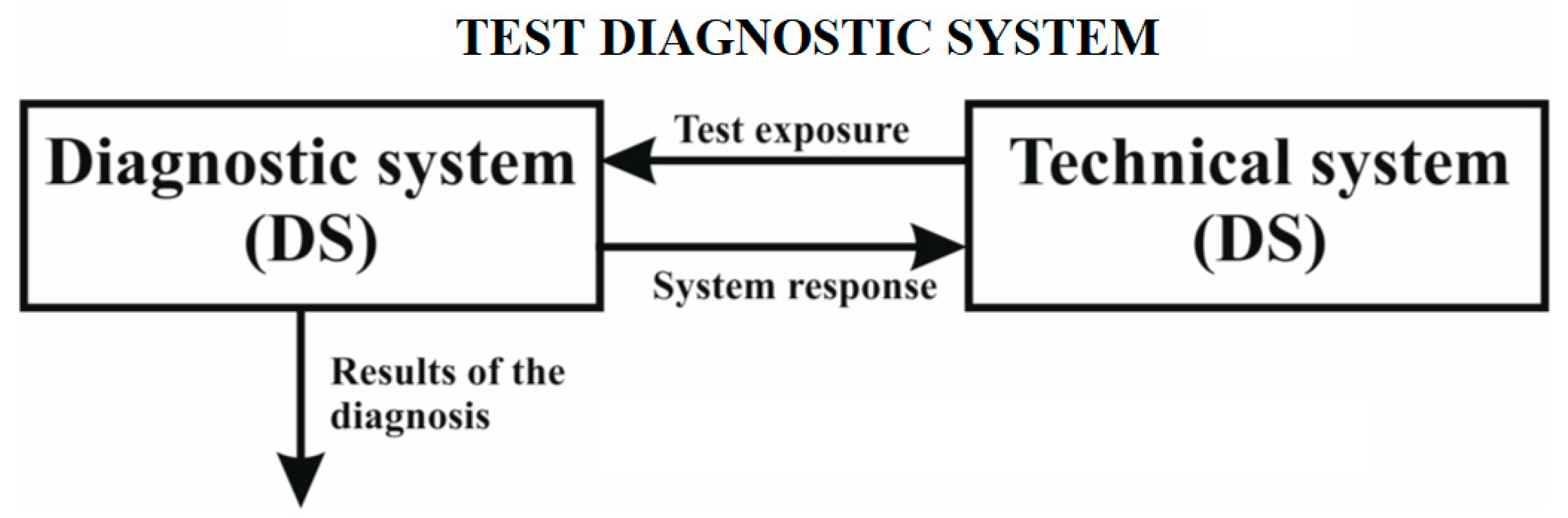
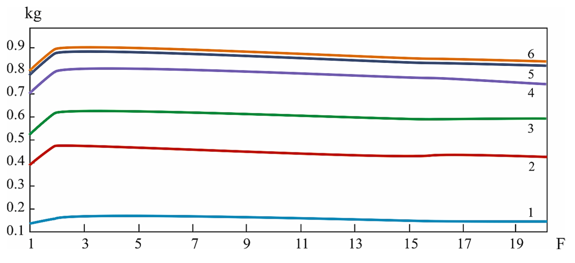
Assessing the Testability of a Technical System

Testability is ensured by distinguishing between defects. During production, operation, and repair, it is possible to accurately determine the fault of a specific module of the object under test. By analysing the test matrix, it is possible to identify the necessary number of additional test points for the differentiation of so-called equivalent defects. Equivalent defects represent faults of the object modules that are indistinguishable using the existing set of test pairs [26,27].

In complex diagnosable systems such as electronic devices or industrial equipment, individual components or blocks are often combined into design units (DUs) to simplify assembly and maintenance. It is useful to place blocks with the same types of potential faults in the same DUs [28]. This allows for the placement of test points (TPs) at the output of each DU, increasing the diagnostic efficiency. The mechanism for selecting test points (TSs) to maximise testability is flexible and most effective when implemented at the system design stage. In complex systems, a large number of TSs may be required, which can lead to complex and expensive hardware as well as delay the diagnosis and troubleshooting process of specific components [29,30]. As additional information, the impact of the hardware implementation of the TS on the testability of the system should be considered [31]. It is important to select technologies and components that provide reliable and accurate fault detection without affecting system performance or functionality. In addition, the diagnostic strategies that will be used to localise faults should be considered. Different diagnostic methods such as testing, monitoring, or the use of artificial intelligence may have different requirements for TSs and their location. Planning the location of TSs should also consider the potential repairability and maintainability of the system [32,33,34]. Access to the TSs should be convenient and without the need to dismantle significant parts of the system. This will allow faults to be quickly identified and repaired, reducing the downtime and maintenance costs [35]. In conclusion, the selection of control points in complex diagnosed systems is a critical factor affecting the testability and reliability of the system. By planning TSs during the design phase, considering hardware implementation, diagnostic strategies and maintenance requirements, it is possible to provide efficient diagnostics, reduce the downtime, and optimise system performance [36,37].

3. Model Description

In the coal industry, modern mines use both manually and automatically controlled mine hoists (MCMHs). The latter operates more carefully in terms of the time spent in the switched-on state [38]. Often, the MCMH is equipped with a diagnostic system (DS). This subsystem allows for the diagnostics (without dismantling and disassembly) of mining equipment [39,40]. For a mine hoist, diagnostics of its mechanical and electrical elements is carried out. The DS performs diagnostics due to the presence of sensors. The use of diagnostic models in the logic circuits of the DS allows the operator to manage the reliability of the equipment on the basis of the obtained data [41].

At the same time, the system must be in a state ready for diagnostics [42,43]. This property is defined as testability. Two approaches are most often used to assess the testability of mining equipment. The first approach is to change the design in order to ensure the ease of carrying out diagnostic procedures [44,45], while the second is to transform the structure of the object without changing its functional properties. The first way is connected with considerable expenses, though it is well-mastered by modern industry. This method does not provide an opportunity to implement a formalised generalised model [46,47,48]. On the other hand, the other path is relatively new. This path is less developed and does not lead to the appearance of significant additional costs for its implementation, which allows one to build formalised models [49,50].

When using this approach, the diagnosed object of the technical system will be represented by a graph of cause–effect relations or in the form of a logic model [51]. The object of the technical system in our work was a mine cargo and passenger hoist (MCPH). Such objects consist of a certain number of related elements [52,53,54]. Even one and the same object of research can be formed from different structures [55,56]. These structures are also not identical, and can have a different number of components [57,58]. The composition of these components can also be different. For modelling purposes, depending on the tasks and needs, these constituent components can be divided into components or vice versa, can be combined.

In our work, we represent the logic model as a directed graph

LM = G (V,U),

(1)

where V is the set of vertices and U is the set of arcs.

The vertices show the blocks that make up the object of study, and the arcs indicate functional relations between them.

In our work, we considered graphs in which arrows were directed from vertices with smaller numbers to vertices with larger numbers. However, in our case, these graphs may be unordered [59,60]. In this case, we optimised the unordered graph. For this purpose, we used the following algorithm of testability optimisation based on the verification matrix:

B = ||b_i,j|| (I = 1, n; j = 1,n).

The generated verification matrix is constructed using certain relations:

b_i,j = 1—in the case when vertex j is included in the check of the i-th control pair;

b_i,j = 0—in the opposite case.

The input and output nodes of a graph constitute verification pairs when their outputs and inputs coincide. Output nodes are inherently checkpoints where information regarding the functioning of the object can be obtained. The number of columns in the verification matrix corresponds to the number of blocks, and the number of rows corresponds to the number of verification pairs. The use of verification matrices in combination with adjacency matrices is effective in analysing complex objects with numerous blocks. This approach allows one to easily identify and analyse the relationships between the input and output nodes, providing a deeper understanding of the functionality and reliability of the system [61].

A square matrix of size (n × n) will be the adjacency matrix of a graph with n vertices

C = ||c_i,j|| (I = 1, n; j = 1,n),

In this square matrix, each element is defined as follows:

c_i,j = 1—if there exists an arc of graph (i,j);

c_i,j = 0—in the opposite case.

In order to determine the depth of diagnosis, let us take the depth of diagnosis as a measure of the depth of fault finding. The following expression [62] will serve to determine the depth of diagnosis:

$$F=\frac{1}{n}{\displaystyle \sum _{r=1}^k{n}_{r}r,}$$

(2)

where n_r is the number of blocks whose defects are searched with depth r. This number of blocks will be determined by the number of r—distinguishable matching columns of the check matrix B_z; n is the total number of blocks in the object and is determined by the number of columns of the check matrix B_z; k is the number of possible classes of defect distinguishability (k < n).

Diagnostic depth (F) is a parameter that characterises the ability of the diagnostic system to localise and identify defects in the diagnostic object. The value of F can vary from 1 to n, where:

-

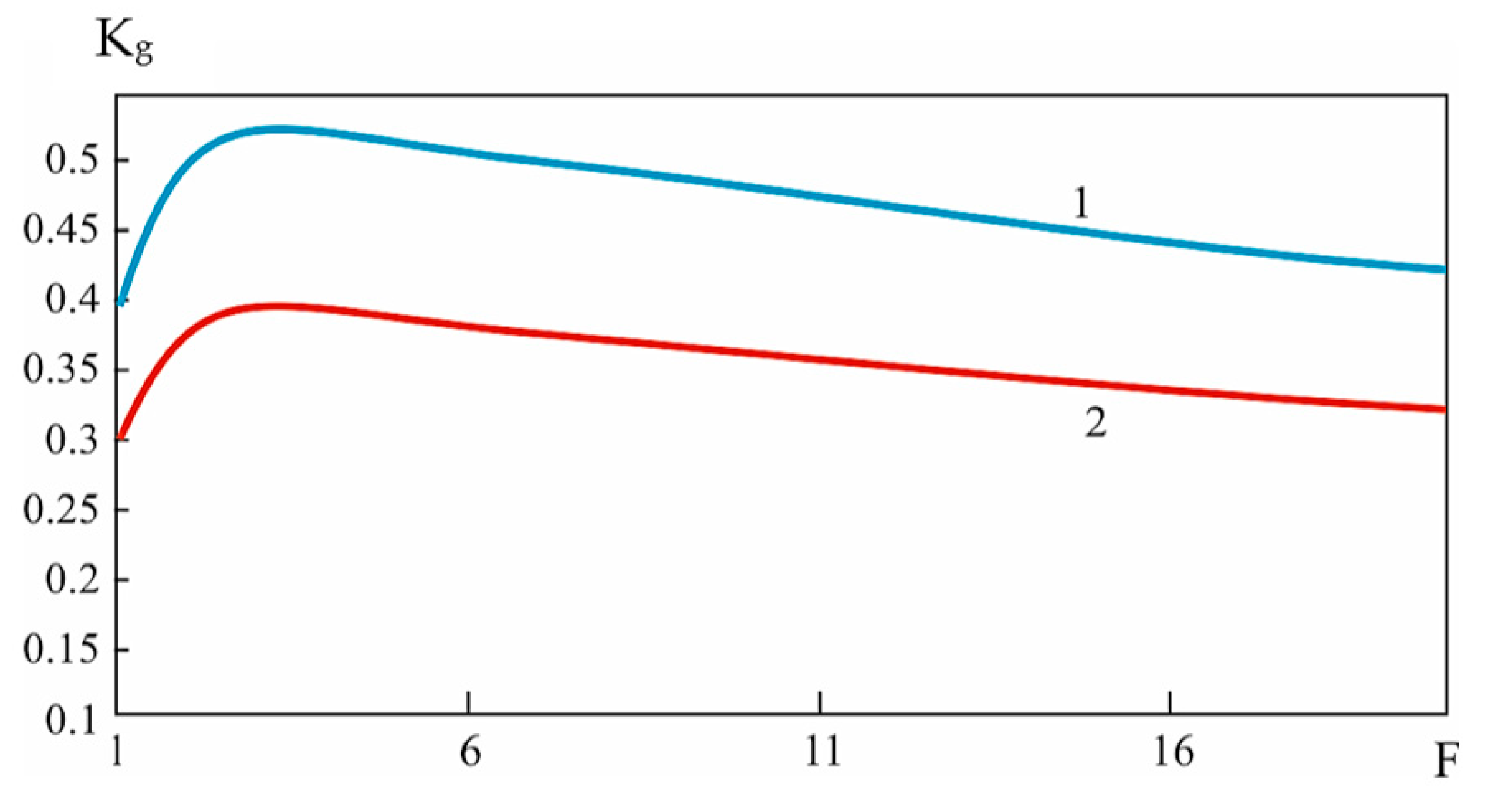
F = 1 corresponds to the minimum level of diagnostics, providing only the indistinguishability of defects;

-

F = n is characteristic of objects with one input and one output, in the case where the exact location of the defect cannot be determined.

The depth of diagnostics is determined by the specifics of the task and the purpose of the system, based on the location of control points during controlled signal discontinuities or the placement of components in structural modules. The optimal number of control points provides the maximum diagnostics for efficient hardware implementation [63,64].

This study analysed diagnostic systems in order to determine the optimal number of test points to guarantee the maximum diagnostic performance and hardware implementation, given the specific requirements and purpose of a system. Testability is a measure of the ability of a diagnostic system to detect and localise defects in an object [65,66]. It depends on the number of control points and their placement. When determining the optimal number of control points, the following factors should be taken into account:

-

The more complex the object, the more control points may be required to achieve the required diagnostic depth.

-

Accessibility of control points. Control points shall be accessible for inspection without the need to disassemble or modify the facility.

-

The cost of adding monitoring points. Adding additional monitoring points can increase the cost of the diagnostic system.

The following methods can be used to determine the optimum number of control points:

-

Graph analysis methods. In this case, the diagnostic object is represented as a graph, where the vertices correspond to the control points and the edges to the possible paths of defect propagation. Graph analysis allows one to determine the minimum number of control points required to achieve a given diagnostic depth.

-

Modelling methods. These methods allow you to simulate the behaviour of a diagnostic system with different numbers of control points and assess its testability.

As a result of the analysis, it was possible to determine the optimal number of control points that provided the required depth of diagnosis with maximum efficiency and minimum cost [67].

Let us define ξ(t) as a random process describing the state of the SNGPD system at time t. Then, the finite number of state variants can be written in the following form:

$$p_i(i)=P_r(\xi (t)=E_i)$$

(3)

At any point in time, the system is in the state $\left(N+1\right)$. This is one of the possible states of the system. At the moment of being in this state, the sum of probabilities of all events that can happen to the system will be equal to one. The transformation of the system between the two states $E_i$ and $E_j$ can be described by a Markov process. $E_i$ is the state of the system at time $t_k$, and $E_j$ at time $t_{k+1}$. At the same time, $p_{ij}$ is the conditional probability of the system being in state $E_j$. Then, the Markov chain will describe our system under study. In this system, the probability of transition between states $E_i$ and $E_j$ does not depend on other factors and only depends on the initial states. This approach makes it possible to predict the behaviour of the system based on its current state. At the same time, this approach does not require considering the previous changes.

We used a square matrix with dimensions $\left(N+1\right)\cdot \left(N+1\right)$ to specify the probability of transition between the states of the system. The elements of this matrix will satisfy the condition $0\le p_{ij}\le 1$ and ${\displaystyle \sum _{i=0}^N{p}_{ij}=1}.$ Let us introduce a transition intensity parameter. This parameter will denote the probabilities of transitions for which time is continuous. Let us introduce the notation $q_{ij}$ for the transition intensity between states $E_i$ and $E_j$. In this case, $q_{ij}$ is defined as the limit of the ratio of the probability of transition of the system between states $E_i$ and $E_j$ for the time interval $\Delta t$ to the length of this interval.

$$q_{ij}\underset{\Delta \to 0}{=}\lim \frac{P_{ij}(\Delta t)}{\Delta t},(i\ne j).$$

(4)

Consider a random process with continuous time, for which the time of being in some state is described by an exponential distribution $F_i(t)=1-e^{-{\lambda }_{i}t}$ where ${\lambda }_i$ is the distribution parameter.

Let us determine the probability of the transition of a random process to another state $E_j$. The initial state will be $E_i$, and the process is in this state for the time $t_0$. The transition time between states is $\Delta t$. This transition process does not depend on the duration of the process being in state $E_t$.

If it is true that the duration of a process in a certain state is described by an exponential distribution with the parameter ${\lambda }_i$, then this exponential distribution will be true for the time from any moment to the moment of state change. The parameter ${\lambda }_i$ will also hold for this distribution. The probability of transition for the time interval $\Delta t$ to another state will be defined as follows:

$$\begin{array}{c}P{i}_j(\Delta t|t\ge t_0)=P_r(t_0\le t\le t_0+\Delta t|t\ge t_0)\\ =\frac{P_r\le t\le t_0+\Delta t}{P_r(t\ge t_0)}=\frac{F(t_0+\Delta t)-F(t_0)}{1-F(t_0)}=1-e^{-{\lambda }_i\Delta t},\end{array}$$

(5)

Let us consider for Expression (5) that the exponential distribution with the parameter ${\lambda }_i$ is true for the whole time of the process being in a certain state and for the time interval between two random moments of time and the moment of transition to another state. Then, the probability for the time $\Delta t$ of the transition to another state will be ${\lambda }_i\Delta t$

$$P{i}_{ij}(\Delta t)=P{i}_{ij}(\Delta t|t\ge t_0)=1-e^{-{\lambda }_i\Delta t}$$

(6)

Let us transform Expression (6) by decomposing the exponent $e-{\lambda }_i\Delta t$ into a series of powers ${\lambda }_i\Delta t$. In this case, we neglected the higher order terms of smallness. Then, (6) will take the following form:

$$P{i}_{ij}(\Delta t)=1-(1-{\lambda }_i\Delta t)\approx {\lambda }_i\Delta t$$

Consider a homogeneous process in which time is continuous. This process will occur in a system having the states $E_0,E_1,\dots ,E_N$.

Calculate the probability $P_i\left(t\right)$ of the system being in state $E_i$ for time t. Add to time t the increment $\Delta t$ and determine the probability of the state at this time: $\left(t+\Delta t\right)$$P_i\left(t+\Delta t\right)$. The transition of the hoisting system at time t to the new state $E_i$ is possible in two ways:

-

The system is already in state $E_i$ and the system has been in this state without making any transitions for the time interval $\Delta t$.

-

The system is in one state $E_j\left(j\ne i\right)$ and has changed state from $E_j$ to $E_i$ and over the time interval $\Delta t$.

The probability for both cases will be different. For the first, it is defined through the product of the probability $P_i\left(t\right)$ and the conditional probability of transition $E_i$ to state $E_j\left(j=0\right)\left(j=0,1,\dots ,i-1,i+1,\dots ,N\right)$. $P_i\left(t\right)$ is the probability of the system being in state $E_i$ at time t. The conditional transition probability is determined by the formula:

$$1-{\displaystyle \sum _{\begin{array}{l}j=0\\ j=1\end{array}}^N{q}_{ij}\Delta t}.$$

(7)

Expression (7) is obtained by considering that $q_{ij}\Delta t$ defines the transition probability between the states of the SNAP system. This is the transition from state $E_i$ to $E_j$ which takes place during time $\Delta t$. The sum of probabilities will give the probability of transition from state $E_t$ to a state other than $E_i$. If we subtract this sum of probabilities from one, we obtain the probability of the reverse event. From this, we can define for the first option the probability as:

$${P_i}^{\left(1\right)}=P_i(t)[1+q_{ij}\Delta t],(i=0,1,\dots ,N)$$

Let us similarly determine the second variant ${P_i}^{\left(2\right)}$. The probability will be equal to the probability $P_j\left(t\right)$ for a fixed state $E_j$, that is, it will be the probability of the system being in state $E_j$ at time t multiplied by the probability of $q_{ij}\Delta t$ moving in time $\Delta t$ to state $E_i:P_j\left(t\right)q_{ij}\Delta t$.

In order to obtain the formula for calculating the total probability, we summed up the value of all probabilities, but excluded the probability of state $E_i$, then:

$$P_i^{\left(2\right)}={\displaystyle \sum _{\begin{array}{l}j=0\\ j=1\end{array}}^N{P}_j(t)q_{ij}\Delta t},\left(i=0,1\dots N\right)$$

(8)

Let us sum the probabilities at time $\left(t+\Delta t\right)$, and then for the probability of state $E_i$, we obtain the expression:

$$P_i\left(t+\Delta t\right)=P^{\left(1\right)}+P^{\left(2\right)}=P_i\left(t\right)\left[1+q_{ii}\Delta t\right]+{\displaystyle \sum _{\begin{array}{l}j=0\\ j=1\end{array}}^N{P}_j(t)q_{ij}\Delta t}$$

(9)

or

$$P_i(t+\Delta t)-P_i(t)={\displaystyle \sum _{i=0}^N{P}_j(t)q{i}_j\Delta t,(i=0,1,\dots ,N).}$$

(10)

Divide the right and left parts of Expression (10) by $\Delta t$ and go to the limit. In this case, $\Delta t\to 0$. As a result, we obtain the following expression:

$$\underset{\Delta \to 0}{\lim }\frac{P_i(t+\Delta t)-P_i(t)}{\Delta t}={\displaystyle \sum _{i=0}^N{P}_j(t)q{i}_j,(i=0,1,\dots ,N).}$$

(11)

For the stable mode of operation of the system, the probabilities of states will tend to infinity. These state probabilities will not depend on the probabilities at the initial time instant. In this stable mode of operation, the derivatives $d{P}_i\left(t\right)/dt=0$. Equating the derivatives to zero changes the general system of differential equations for the steady-state regime. It can be represented in this case as:

$${\displaystyle \sum _{j=0}^N{P}_i(t)q_{ij}=0,}(i=0,1,\dots ,N),$$

(12)

Taking into account that ${\displaystyle \sum _{i=0}^N{P}_i=1,}$ we will have a single solution for the system of equations.

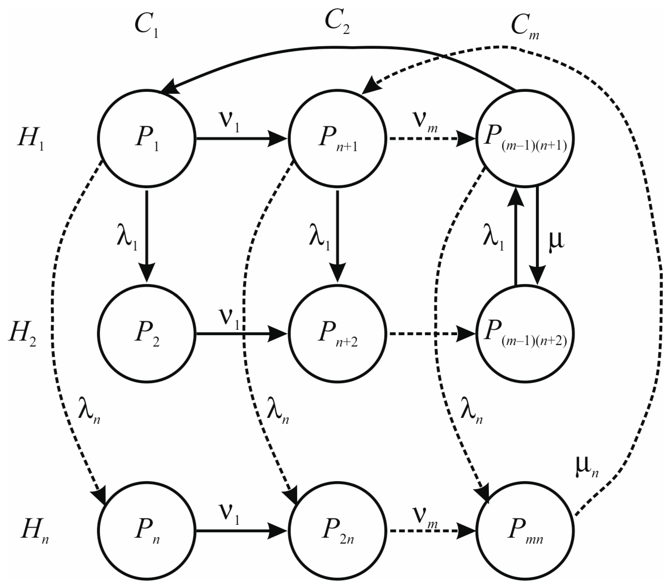
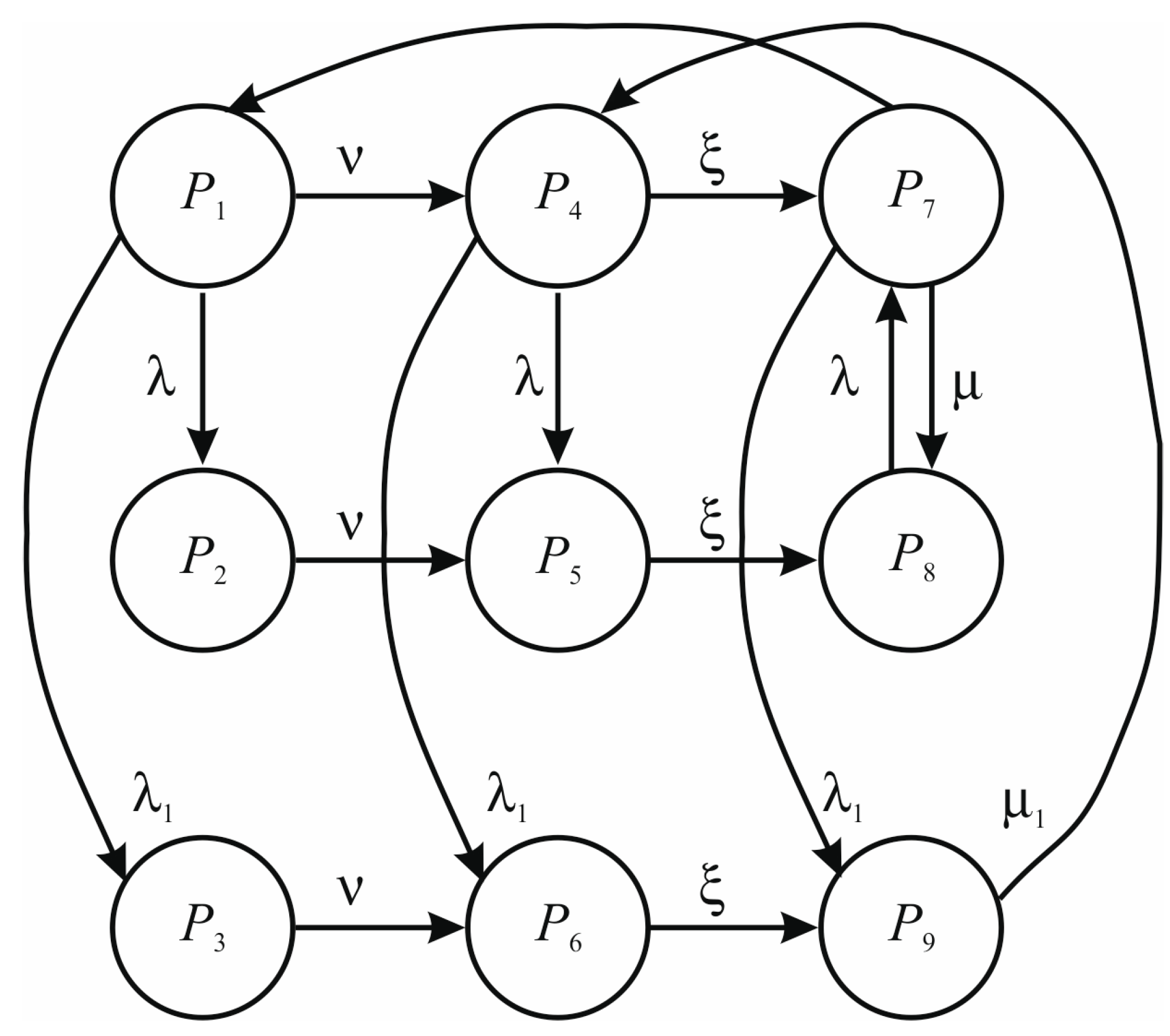
4. Formation of the Transition Graph for Description of Variants of Use of the System of Diagnostics of the Technical System

The ways of connecting diagnostic systems (DSs) to the MCMH system can be quite diverse. The components of the DS are sensors, signal normalisers, switchboard, information processing devices registration and indication units [68,69]. Depending on the location of these components, we can distinguish different structures of DSs with DSs. The authors introduced the concept of an inbuilt technical diagnostics tool that was an integral part of the object, and an external technical diagnostics tool that was structurally separate from the object [70]. Intermediate variants are possible when separate elements of the DS can be located in the object [71,72]. In practice, the variety of connection methods can be caused by the design features of the DSs, where DSs will work more effectively either in the built-in version or with built-in separate components. The influence of interference and electromagnetic interference on the measurement accuracy is of great importance when placing the DSs. It is necessary to consider that in the analysis of the testability of MCMH systems, equivalent defects are revealed, therefore, a part of the blocks is concentrated in separate constructive units. The economic factor is also of great importance, as different configurations can have different costs [73,74,75]. It is possible to distinguish a general approach, which allows for the analysis of the reliability of the DS of MCMH systems.

Figure 2 shows the state graph for the technical system (TS) with a DS for the general case of the placement of individual components of the DS in the TS. The proposed approach allows a general model to be built for the analysis and optimisation of reliability indicators.

The horizontal columns of the graph represent the states C_m, corresponding to the operating modes of the MCMH and DS. These modes include the operation of the MCMH system and verification of the monitored MCMH and DS. In practice, other modes may also be used.

The vertical lines of the graph correspond to the states H₁, …, H_n, in which the elements of the SNAP system and the DS can be located. The number of these states depends on the number of components of the DS and the MCMH system to be checked. These can be sensor groups, individual sensors, switches, processing units, displays, and indicators.

The scheme uses the following designations: λ_n—probability of failure of the elements selected for diagnostics; ν_m—probability of switching to the control mode of the corresponding element; μ_n—probability of recovery of this element; η—probability of returning to the operating mode; P_k—probability of finding the MCMH system with DS in one of the specified states.

The system of equations of discrete processes with continuous time looks like this:

$${\displaystyle \sum _{k=1}^{mn}{\displaystyle \sum _{j=1}^m{\displaystyle \sum _{i=1}^n{P}_k{q}_{ij}=0.}}}$$

(13)

By taking the normalising condition into account and solving this system of equations, we are able to determine the probabilities. The availability factor is determined by these probabilities. There is another option to solve the problem of testing diagnostic systems and increasing the availability factor. It is possible to separate the diagnostic and technical systems of the MCMH (Figure 3).

The graph of the structure, which separates the diagnostic system from the technical system, is shown in Figure 4. The technical system includes information processing devices, sensors, and switches. The diagnostic system includes indication and registration units. Information transfer between these systems is carried out by means of communication channels. Possible states of the system are shown in the graph (Figure 4). The different states are labelled by the letter P with an index. P is the probability of being in operation or test mode with different states of the diagnostic system and the technical system.

• P₁—the system is working, DS and TS are in good working order;
• P₂—the system works, the TS is faulty;
• P₃—the system is operational, the DS is faulty;
• P₄—the system is in the DS test mode, DS and TS are OK;
• P₅—the system is in the DS test mode, the TS is faulty;
• P₆—the system is in the DS test mode, DS is faulty;
• P₇—the system is in the TS test mode, DS and TS are OK;
• P₈—the system is in the TS test mode, TS is faulty;
• P₉—the system is in the TS test mode, the DS is faulty.

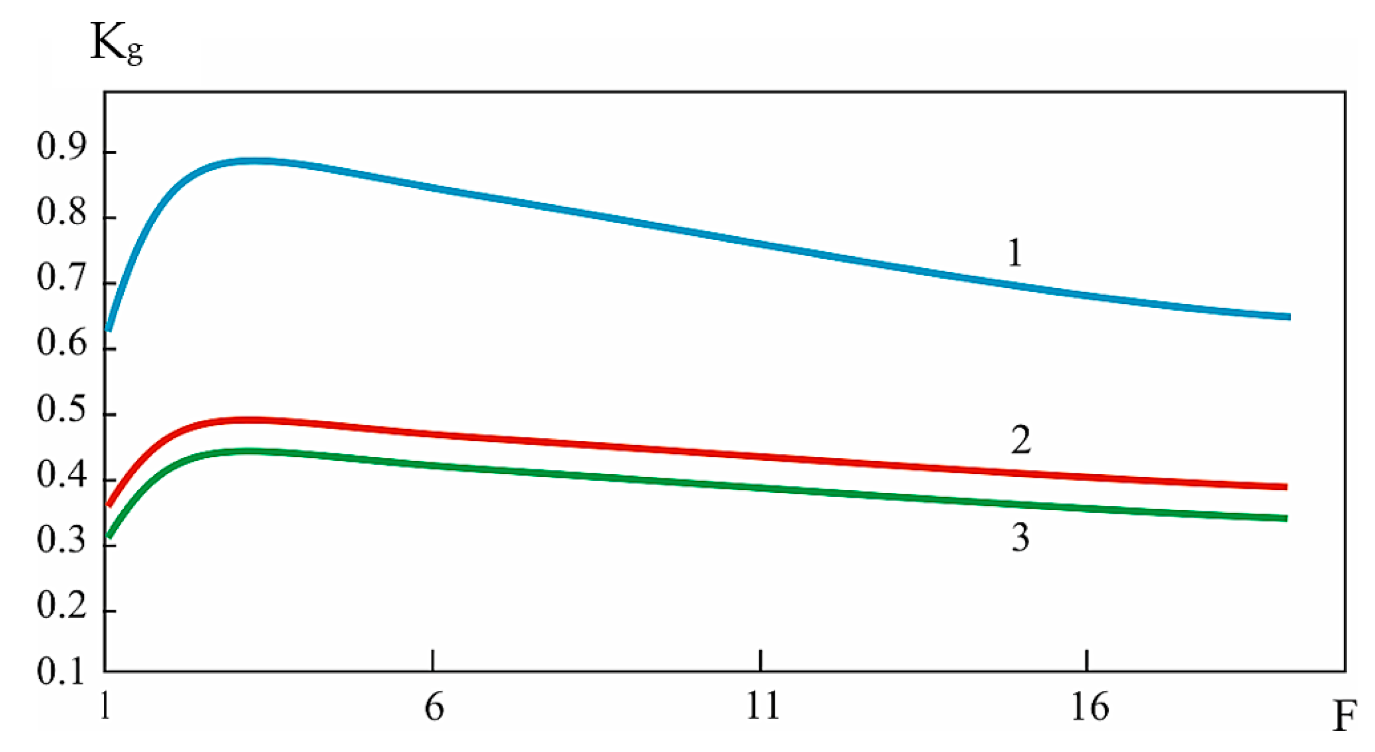
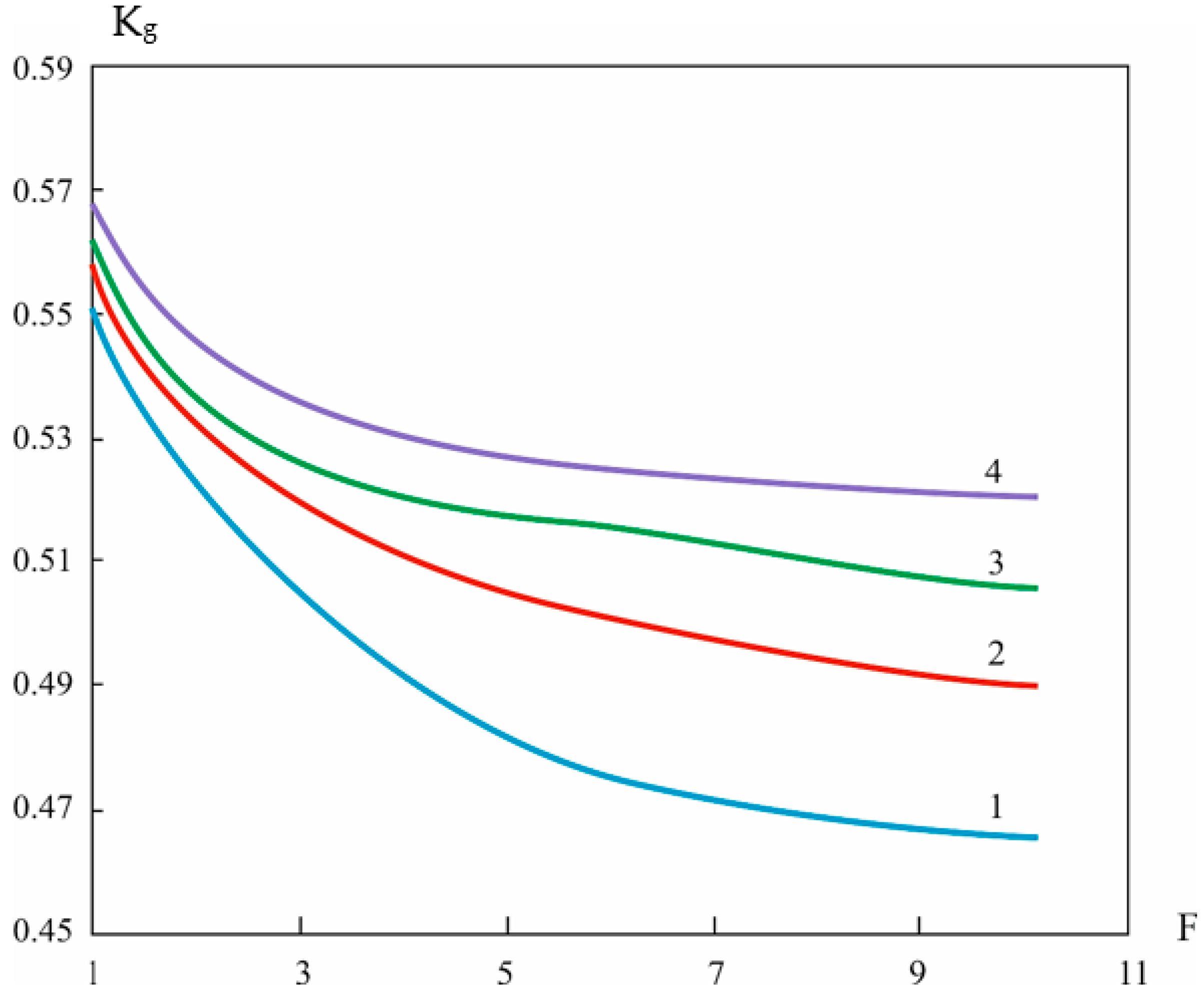
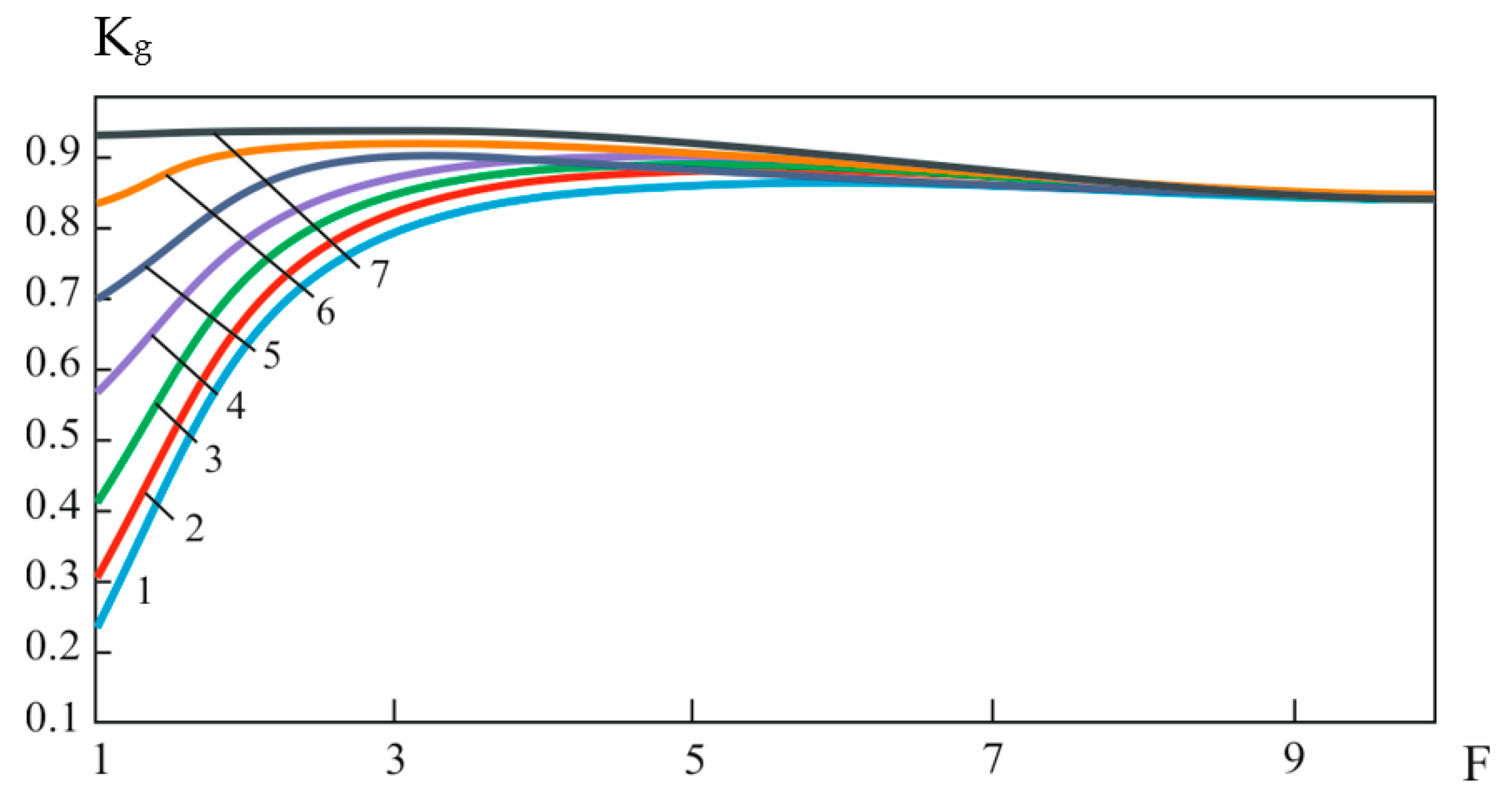
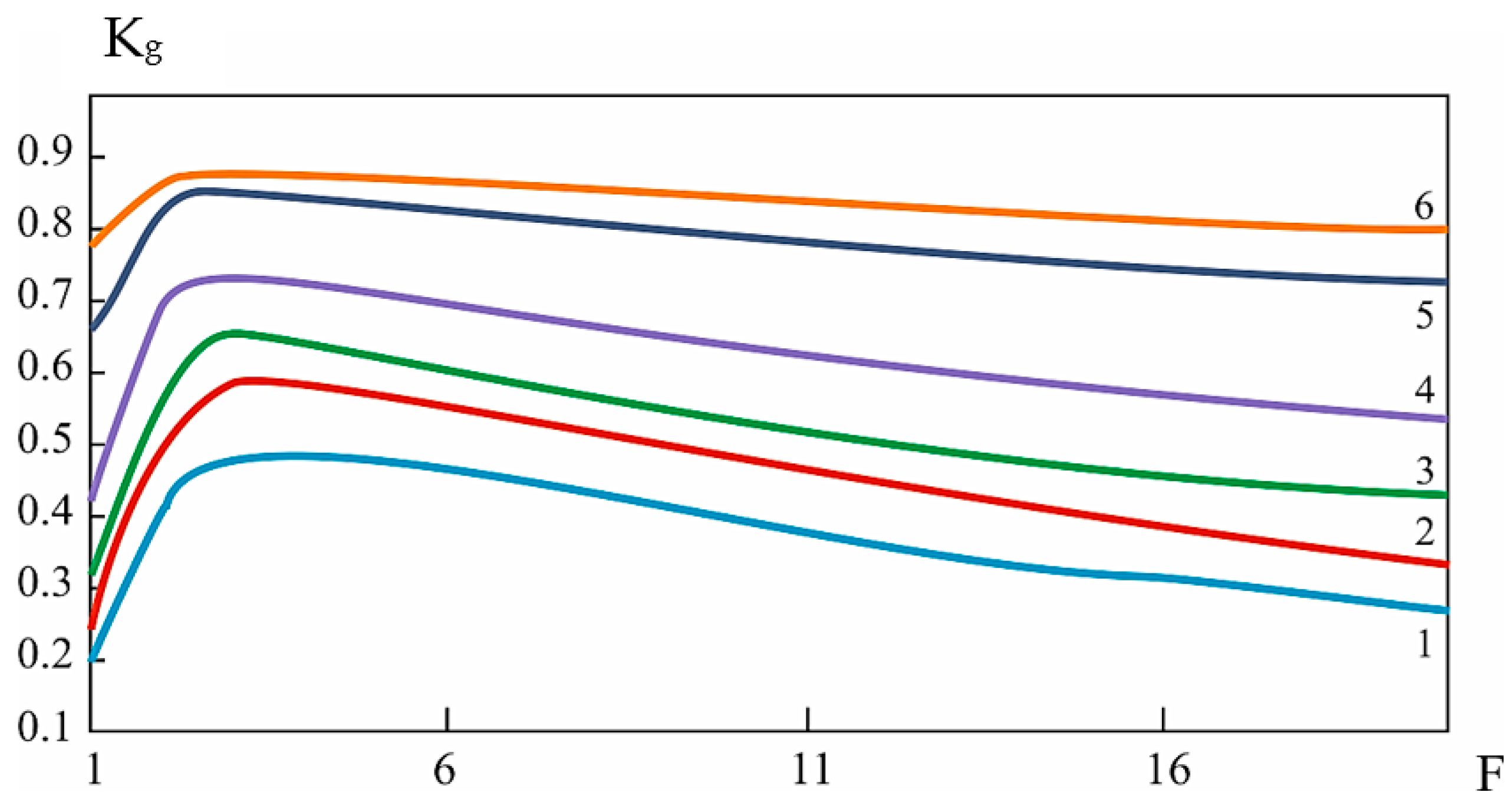
It is also important to consider that a system can be in various combinations of these states, which affects its overall performance and reliability:

P₁ + P₂ + P₃ + P₄ + P₅ + P₆ + P₇ + P₈ + P₉ = 1.

(14)

The corresponding system of equations for the nine states of the SNAP system with an external diagnostic system is as follows:

$$\left.\begin{array}{l}\begin{array}{l}\begin{array}{l}-\left(\lambda +{\lambda }_1+\nu \right)P_1+\eta P_7=0\\ \lambda P_1-v{P}_2=0\end{array}\hfill \\ {\lambda }_1{P}_1-v{P}_3=0\hfill \\ \begin{array}{l}v{P}_1-\left(\xi +\lambda +{\lambda }_1\right)P_4+{\mu }_1{P}_9=0\\ v{P}_2+\lambda P_4-\xi P_5=0\end{array}\hfill \\ v{P}_3+{\lambda }_1{P}_4-\xi P_6=0\hfill \\ \begin{array}{l}\xi P_4+\mu P_8-\left(\lambda +{\lambda }_1+\eta \right)P_7=0\\ \xi P_5+\lambda P_7-\mu P_8=0\end{array}\hfill \end{array}\\ \xi P_6+{\lambda }_1{P}_7-{\mu }_1{P}_9=0\end{array}\right\}.$$

(15)

For this case, the availability factor and the idle factor are respectively equal:

K_g = P₁ + P₃,

(16)

K_np = 1 − K_g.

(17)

Based on the results obtained, it can be said that there is no universal way to connect diagnostic equipment [76,77,78]. Each specific case is unique and requires its own optimal method [79,80].

5. Discussion

The comparison of the reliability level of the used methods of placing the system of the mine cargo-passenger hoist showed the change in values of the system availability factor in a wide enough interval. The value of change of this coefficient largely depends on the parameters of the object. This is true for various methods and allows one to say that a universal and effective method cannot be singled out. For each specific condition and parameter of the research object, any of the considered methods can be optimal. For some conditions, one method will be optimal, and for others, another method will be optimal. As a result, for each case, a different method of DS placement in the MCMH is suitable, which will be optimal in technical terms. In the previous section, we provided formulas for calculating the optimal value of the diagnostic depth F. At this value of F, the minimum value of recovery time T will be achieved T_β.

The recovery intensity value has an inverse dependence on the recovery time. Based on this, we can say that there is a maximum value of recovery intensity and availability factor K_g. For further reliability analysis, we plotted the dependences of the availability factor on the parameters of the mine hoist. Among these parameters were the diagnostic depths, inspection intensity, etc. However, the most important, from the point of view of system reliability, is the analysis of the dependences of the idle ratio K_np on the depth of diagnosing F and of the readiness coefficients K_g on the depth of diagnosing F. These dependences are shown in Figure 5 and Figure 6. The dependences are shown for different values of parameter α, which considers the complexity of the object.

The dependences presented in Figure 5 and Figure 6 have minima and maxima. These extrema are clearly expressed. The influence of the structural parameter α on the values of the coefficients K_g and K_np is also clearly visible. When analysing the reliability of systems, as a rule, the increase in the complexity of the object leads to a decrease in the reliability of its operation and increases the probability of failures. In this case, a similar dependence is observed for the structural parameter α. The growth in the values of this parameter leads to a decrease in the values of the availability factor, and vice versa, where the growth in the values of diagnostic depth leads to the growth in the availability factor values. These dependences are true for all four ways of diagnostics system (DS) placement. The dependence is maintained, although the numerical values will be different.

Expressions for determining the derivatives of the availability and downtime factors allow for the optimum value of the diagnostic depth to be calculated. These expressions are derived for the integrated diagnosis system. If these expressions are equated to zero, the optimum values can be determined. The optimum value for the availability factor K_g is the maximum value. For the idle factor K_np, the optimum value is the minimum value. Calculating the values of these coefficients analytically is a rather complex and difficult task. Figure 7 shows that the value of the maximum availability factor depends on the complexity of the object. An increase in complexity leads to a decrease in the value of the maximum coefficient. Similarly, the growth in the value of the initial depth of diagnostics F₀ leads to its decrease. On this basis, the dependence K_g (F) is extremely important in the case of changing values of the initial depth of diagnostics [80]. This dependence (Figure 8) allows one to determine the optimal value for the diagnostic depth F_opt. This optimal value of F_opt will provide the maximum value of the availability factor. The relationship between F_opt and the value of the diagnostic depth F will play an important role in analysing and improving the reliability of the system. The value of F is obtained by analysing the inspection matrix for equivalent defects.

The depth of diagnostics required for diagnostics at the initial stage F₀ will be determined when designing the object with control points. The dependence of the readiness factor on the diagnostic depth for different numbers of test points is shown in Figure 8. This figure shows that in the case where F_onm < F₀, it is necessary to reduce the value of F by introducing additional control points. This makes it possible to break down the localisation of defects and the classes of equivalent defects. In this case, the reduction in the value of the diagnostic depth is limited to the value of the optimal diagnostic depth; F cannot be smaller.

In the opposite case, when F_onm > F₀, the number of control points should be reduced. This will decrease the value of T_β. The analysis of the obtained results also showed other dependencies and regularities. An increase in the value of the complexity coefficient α naturally results in an increase in F_opt. There was a similar dependence for the search time τ₀, where the more τ₀, the more F_opt.

The data in the graphs show important dependencies. The availability factor depends to a large extent on the failure rate values. Reducing the failure rate increases the reliability of the equipment and increases the availability. Graphs confirming this are presented in Figure 9 and Figure 10. These graphs show that the selection of values of diagnostic intensity allows one to change the availability factor. However, from the same graphs, it is clear that the degree of influence depends on the value of the diagnostic cycle frequency ξ. At values ξ > 5 (Figure 9), the growth rate of the readiness factor slows down when changing the values of the diagnostic intensity. Knowing this, it is possible to select the values of the diagnostic cycle frequency, which will allow one to obtain the necessary value of the availability factor. A similar analysis can be performed for Figure 11. The data presented in this graph suggest that there is an optimum value of the frequency of control of the SNAP system. At this frequency, the maximum value will be obtained by the availability factor. This is very important to obtain the maximum reliability of the operating equipment [59].

The performed research on the modelling and reliability assessment of the MCMH operation allowed us to determine the optimal values of a number of parameters. The optimal value of diagnostics depth was determined. At this value, the maximum availability factor is obtained. The dependence on the system parameters was obtained for the availability factor.

The development of a model of reliability of operation for the object of study was carried out in the form of a transition graph in combination with a system of equations. The obtained system of equations allowed us to assess the reliability of the MCMH with DS. Additionally, the developed model allows one to determine the readiness (using the readiness factor) and downtime of the elements of the MCMH with a DS. This paper shows the dependence of the readiness of the object under study for diagnostics on the system parameters. We investigated the influence of various parameters of the MCMH system with DS. Among these parameters were the troubleshooting time, the failure rate, monitoring intensity of the diagnosis system, etc. The obtained model showed the causal relationship between the elements of the MCMH and allowed us to obtain the maximum value of the availability factor and the depth of possible diagnostics for this value of the availability factor. With the use of this model, a methodology for assessing the reliability of mine equipment on the example of a MCMH was developed This methodology can be integrated into the operation of equipment to reduce the probability of failure of equipment elements and increase the reliability of its operation as a whole.

The authors consider the topic to be original research and relevant in the field of the assessment and improvement in the reliability of mining equipment. It concerns quite a wide area—the reliability of mining equipment, power engineering, and mining transportation. Additionally, this reliability model can be developed and applied in other areas of industry.

The proposed mathematical logic model for analysing the controllability of mining equipment, taking into account its resource and diagnostic parameters including testability, correlates with the general reliability models described in [65,67,80,81], which allows us to speak about its adequacy and applicability to the analysis of mining equipment.

As a result of compiling the reliability model, the authors drew the following conclusions concerning the testability of equipment. After reliability modelling, the property of the object, which characterises its adaptability to control and technical diagnostics, is the testability of the object. The efficiency of diagnostics task solutions depends on whether the given object possesses controllability properties or not. It also means the minimisation of all costs and expenses connected with the organisation of control and technical diagnostics and leads to an improvement in operational characteristics. Without solving the issues of testability, the application of special methods and automated means of diagnostics can be ineffective. In this connection, an approach to bring the object to the controllability is proposed, which consists of the following. The testability property of the object of diagnostics is formed at the stage of its design, where the interrelationship is established. At the stage of its design, where interrelations and parameters of the object are established, the essence, variety, and character of these relations are revealed and the object of diagnostics is represented through the received interrelations (i.e., in essence there is a construction of an effective model of the diagnosed object).

6. Conclusions

As a result of the conducted scientific research and instrumental observations, the following tasks were solved:

• The method of determining the reliability of mine hoisting installations and increasing their testability was proposed;
• The dependence of the availability factor on various parameters of the technical system of the mine hoisting plant was analysed in order to ensure normative reliability;
• A methodology for assessing the reliability of mine hoisting plants was developed that includes effective ways to improve the reliability of plant operation by using technological measures.

A mathematical model for the system of a mine hoisting plant with an external diagnostic system was developed. This model was realised in the form of a transition graph. The graph was supplemented with a system of equations to assess the reliability of the system. The methods presented in this paper allowed us to determine the maximum availability factor by achieving the optimal values of the diagnostic depth. A methodology for assessing the reliability of mine hoisting systems was developed.

The practical significance of the work is as follows:

• A mathematical model of a mine hoisting plant was developed in order to analyse its reliability as a complex technical system with different depths of diagnostics;
• The dependence of the availability factor on various parameters of the technical system of the mine hoisting plant was analysed in order to ensure normative reliability;
• A methodology for assessing the reliability of mine hoisting plants was proposed including effective ways to improve the reliability of operation of both individual elements and the whole plant through the use of technological measures.

The practical value of the work consists of the development of a methodology for assessing the reliability of mine hoisting plants in order to increase the plant availability factor. The work shows a universal block in the realisation of the diagnostics process, which is aimed at controlling the functioning of mine equipment and in particular, mine hoisting plants. Control was carried out by obtaining information from sensors in analogue form while sensors were located in control points.

References

1. Dhillon, B.S. Mining Equipment Reliability, Maintainability, and Safety; Springer: London, UK, 2008. [Google Scholar]
2. Carlo, F.D. Reliability and Maintainability in Operations Management; Massimiliano, S., Ed.; InTech: London, UK, 2013. [Google Scholar]
3. Abramovich, B.N.; Bogdanov, I.A. Improving the efficiency of autonomous electrical complexes of oil and gas enterprises. J. Min. Inst. 2021, 249, 408–416. [Google Scholar] [CrossRef]
4. Kumar, U.; Klefsjo, B. Reliability analysis of hydraulic systems of LHD machines using the power law process model. Reliab. Eng. Syst. Saf. 1992, 35, 217–224. [Google Scholar] [CrossRef]
5. Troy, D. The Importance of Efficient Mining Equipment. Available online: https://industrytoday.com/importance-efficientmining-equipment/ (accessed on 12 February 2023).
6. Amy, H. What Is Equipment Reliability and How Do You Improve It? Available online: https://nonstopreliability.com/equipment-reliability/ (accessed on 15 October 2020).
7. Meshkov, A.A.; Kazanin, O.I.; Sidorenko, A.A. Improving the efficiency of the technology and organisation of the longwall face move during the intensive flat-lying coal seams mining at the kuzbass mines. J. Min. Inst. 2021, 249, 342–350. [Google Scholar] [CrossRef]
8. Nazarychev, A.N.; Dyachenok, G.V.; Sychev, Y.A. A reliability study of the traction drive system in haul trucks based on failure analysis of their functional parts. J. Min. Inst. 2023, 261, 363–373. [Google Scholar]
9. Norris, G. The True Cost of Unplanned Equipment Downtime. Available online: https://www.forconstructionpros.com/equipment-management/article/21104195/the-true-cost-of-unplanned-equipment-downtime (accessed on 3 December 2019).
10. Kumar, U. Reliability Analysis of Load-Haul-Dump Machines. Ph.D. Thesis, Lulea Tekniska Universitet, Lulea, Sweden, 1990. [Google Scholar]
11. Provencher, M. A Guide to Predictive Maintenance for the Smart Mine. Available online: https://www.mining.com/a-guide-to-predictive-maintenance-for-the-smart-mine/ (accessed on 16 April 2020).
12. Sellathamby, C.; Moore, B.; Slupsky, S. Increased Productivity by Condition-Based Maintenance Using Wireless Strain Measurement System. In Proceedings of the Canadian Institute of Mining (CIM) MEMO Conference, Sudbury, ON, Canada, 24–27 October 2010. [Google Scholar]
13. Glazunov, V.V.; Burlutsky, S.B.; Shuvalova, R.A.; Zhdanov, S.V. Improving the reliability of 3D modelling of a landslide slope based on engineering geophysics data. J. Min. Inst. 2022, 257, 771–782. [Google Scholar] [CrossRef]
14. Koteleva, N.; Korolev, N. A Diagnostic Curve for Online Fault Detection in AC Drives. Energies 2024, 17, 1234. [Google Scholar] [CrossRef]
15. Vasilyeva, N.; Golyshevskaia, U.; Sniatkova, A. Modeling and Improving the Efficiency of Crushing Equipment. Symmetry 2023, 15, 1343. [Google Scholar] [CrossRef]
16. Zakharchenko, A.I.; Leusenko, Y.A. A comprehensive approach to solution of the problem of improving the quality of mine equipment. Ugol’Ukr. (Ukr. SSR) 1980, 7, 16–17. [Google Scholar]
17. Viray, F.L. Coal Mine Productivity Assessment as Influenced by Equipment Reliability and Availability; ProQuest Dissertations Publishing: Ann Arbor, MI, USA, 1982; p. 338. [Google Scholar]
18. Nevskaya, M.A.; Raikhlin, S.M.; Vinogradova, V.V.; Belyaev, V.V.; Khaikin, M.M. A Study of Factors Affecting National Energy Efficiency. Energies 2023, 16, 5170. [Google Scholar] [CrossRef]
19. Zhukovskiy, Y.; Buldysko, A.; Revin, I. Induction Motor Bearing Fault Diagnosis Based on Singular Value Decomposition of the Stator Current. Energies 2023, 16, 3303. [Google Scholar] [CrossRef]
20. Stanek, E.; Venkata, S. Mine power system reliability. IEEE Trans. Ind. Appl. 1988, 24, 827–838. [Google Scholar] [CrossRef]
21. Collins, E.W. Safety evaluation of coal mine power systems. In Proceedings of the Annual Reliability and Maintainability Symposium, Philadelphia, PA, USA, 27 January 1987; Sandia National Labs.: Albuquerque, NM, USA, 1987. [Google Scholar]
22. Samanta, B.; Sarkar, B.; Mukherjee, S.K. Reliability assessment of hydraulic shovel system using fault trees. Min. Technol. Trans. Inst. Min. Metall. Sect. A 2002, 111, 129–135. [Google Scholar] [CrossRef]
23. Kunshin, A.; Dvoynikov, M.; Timashev, E.; Starikov, V. Development of Monitoring and Forecasting Technology Energy Efficiency of Well Drilling Using Mechanical Specific Energy. Energies 2022, 15, 7408. [Google Scholar] [CrossRef]
24. Abdollahpour, P.; Tabatabaee Moradi, S.S.; Leusheva, E.; Morenov, V. A Numerical Study on the Application of Stress Cage Technology. Energies 2022, 15, 5439. [Google Scholar] [CrossRef]
25. Coetzee, J.L. The role of NHPP models in the practical analysis of maintenance failure data. Reliab. Eng. Syst. Saf. 1997, 56, 161–168. [Google Scholar] [CrossRef]
26. Tynchenko, V.S.; Bukhtoyarov, V.V.; Wu, X.; Tyncheko, Y.A.; Kukartsev, V.A. Overview of Methods for Enhanced Oil Recovery from Conventional and Unconventional Reservoirs. Energies 2023, 16, 4907. [Google Scholar] [CrossRef]
27. Malozyomov, B.V.; Martyushev, N.V.; Voitovich, E.V.; Kononenko, R.V.; Konyukhov, V.Y.; Tynchenko, V.; Kukartsev, V.A.; Tynchenko, Y.A. Designing the Optimal Configuration of a Small Power System for Autonomous Power Supply of Weather Station Equipment. Energies 2023, 16, 5046. [Google Scholar] [CrossRef]
28. Malozyomov, B.V.; Martyushev, N.V.; Konyukhov, V.Y.; Oparina, T.A.; Zagorodnii, N.A.; Efremenkov, E.A.; Qi, M. Mathematical Analysis of the Reliability of Modern Trolleybuses and Electric Buses. Mathematics 2023, 11, 3260. [Google Scholar] [CrossRef]
29. Efremenkov, E.A.; Valuev, D.V.; Qi, M. Review Models and Methods for Determining and Predicting the Reliability of Technical Systems and Transport. Mathematics 2023, 11, 3317. [Google Scholar] [CrossRef]
30. Zuo, X.; Yu, X.R.; Yue, Y.L.; Yin, F.; Zhu, C.L. Reliability Study of Parameter Uncertainty Based on Time-Varying Failure Rates with an Application to Subsea Oil and Gas Production Emergency Shutdown Systems. Processes 2021, 9, 2214. [Google Scholar] [CrossRef]
31. Kumar, N.S.; Choudhary, R.P.; Murthy, C. Reliability based analysis of probability density function and failure rate of the shovel-dumper system in a surface coal mine. Model. Earth Syst. Environ. 2020, 7, 1727–1738. [Google Scholar] [CrossRef]
32. Balaraju, J.; Raj, M.G.; Murthy, C. Estimation of reliability-based maintenance time intervals of Load-Haul Dumper in an underground coal mine. J. Min. Environ. 2018, 9, 761–771. [Google Scholar]
33. Barabady, J.; Kumar, U. Reliability analysis of mining equipment: A case study of a crushing plant at Jajarm Bauxite Mine in Iran. Reliab. Eng. Syst. Saf. 2008, 93, 647–653. [Google Scholar] [CrossRef]
34. Taherı, M.; Bazzazı, A.A. Reliability Analysis of Loader Equipment: A Case Study of a Galcheshmeh. J. Undergr. Resour. 2017, 11, 37–46. Available online: https://dergipark.org.tr/en/pub/mtb/issue/32053/354893 (accessed on 3 March 2022).
35. Bala, R.J.; Govinda, R.; Murthy, C. Reliability analysis and failure rate evaluation of load haul dump machines using Weibull. Math. Model. Eng. Probl. 2018, 5, 116–122. [Google Scholar] [CrossRef]
36. Waghmode, L.Y.; Patil, R.B. Reliability analysis and life cycle cost optimisation: A case study from Indian industry. Int. J. Qual. Reliab. Manag. 2016, 33, 414–429. [Google Scholar] [CrossRef]
37. Hoseinie, S.H.; Ataei, M.; Khalokakaie, R.; Ghodrati, B.; Kumar, U. Reliability analysis of the cable system of drum shearer using the power law process model. Int. J. Min. Reclam. Environ. 2012, 26, 309–323. [Google Scholar] [CrossRef]
38. Roy, S.K.; Bhattacharyya, M.M.; Naikan, V.N. Maintainability and reliability analysis of a fleet of shovels. Min. Technol. Trans. Inst. Min. Metall. Sect. A 2001, 110, 163–171. [Google Scholar] [CrossRef]
39. Ilyushina, A.N.; Pershin, I.M.; Trushnikov, V.E.; Novozhilov, I.M.; Pervukhin, D.A.; Tukeyev, D.L. Design of Induction Equipment Complex using the Theory of Distributed Parameter Systems. In Proceedings of the 2023 5th International Conference on Control in Technical Systems (CTS 2023), St. Petersburg, Russia, 26–28 September 2023; pp. 79–82. [Google Scholar] [CrossRef]
40. Skamyin, A.N.; Dobush, I.V.; Gurevich, I.A. Influence of nonlinear load on the measurement of harmonic impedance of the power supply system. In Proceedings of the 2023 5th International Youth Conference on Radio Electronics, Electrical and Power Engineering (REEPE 2023), Moscow, Russia, 16–18 March 2023. [Google Scholar] [CrossRef]
41. Hall, R.A.; Daneshmend, L.K. Reliability Modelling of Surface Mining Equipment: Data Gathering and Analysis Methodologies. Int. J. Surf. Min. 2003, 17, 139–155. [Google Scholar] [CrossRef]
42. Ascher, H.; Feingold, H. Repairable Systems Reliability: Modeling, Inference, Misconceptions and Their Causes; Marcel Dekker, Inc.: New York, NY, USA, 1984. [Google Scholar]
43. Malozyomov, B.V.; Martyushev, N.V.; Sorokova, S.N.; Efremenkov, E.A.; Qi, M. Mathematical Modeling of Mechanical Forces and Power Balance in Electromechanical Energy Converter. Mathematics 2023, 11, 2394. [Google Scholar] [CrossRef]
44. Golik, V.I.; Brigida, V.; Kukartsev, V.V.; Tynchenko, Y.A.; Boyko, A.A.; Tynchenko, S.V. Substantiation of Drilling Parameters for Undermined Drainage Boreholes for Increasing Methane Production from Unconventional Coal-Gas Collectors. Energies 2023, 16, 4276. [Google Scholar] [CrossRef]
45. Martyushev, N.V.; Malozyomov, B.V.; Sorokova, S.N.; Efremenkov, E.A.; Qi, M. Mathematical Modeling the Performance of an Electric Vehicle Considering Various Driving Cycles. Mathematics 2023, 11, 2586. [Google Scholar] [CrossRef]
46. Klyuev, R.V.; Karlina, A.I. Improvement of Hybrid Electrode Material Synthesis for Energy Accumulators Based on Carbon Nanotubes and Porous Structures. Micromachines 2023, 14, 1288. [Google Scholar] [CrossRef]
47. Rao, K.R.; Prasad, P.V. Graphical methods for reliability of repairable equipment and maintenance planning. In Proceedings of the Annual Symposium on Reliability and Maintainability (RAMS), Philadelphia, PA, USA, 22–25 January 2001; pp. 123–128. [Google Scholar]
48. Kumar, R.; Vardhan, A.; Kishorilal, D.B.; Kumar, A. Reliability analysis of a hydraulic shovel used in open pit coal mines. J. Mines Met. Fuels 2018, 66, 472–477. [Google Scholar]
49. Sinha, R.S.; Mukhopadhyay, A.K. Reliability centred maintenance of cone crusher: A case study. Int. J. Syst. Assur. Eng. Manag. 2015, 6, 32–35. [Google Scholar] [CrossRef]
50. Ruijters, E.; Stoelinga, M. Fault Tree Analysis: A survey of the state-of-the-art in modelling, analysis and tools. Comput. Sci. Rev. 2015, 15–16, 29–62. [Google Scholar] [CrossRef]
51. Yong, B.; Qiang, B. Subsea Engineering Handbook; Gulf Professional Publishing: Oxford, UK, 2018. [Google Scholar]
52. Singh, R. Pipeline Integrity Handbook; Gulf Professional Publishing: Oxford, UK, 2017. [Google Scholar]
53. Gharahasanlou, A.N.; Mokhtarei, A.; Khodayarei, A.; Ataei, M. Fault tree analysis of failure cause of crushing plant and mixing bed hall at Khoy cement factory in Iran. Case Stud. Eng. Fail. Anal. 2014, 2, 33–38. [Google Scholar] [CrossRef]
54. Kang, J.; Sun, L.; Soares, C.G. Fault Tree Analysis of floating offshore wind turbines. Renew. Energy 2019, 133, 1455–1467. [Google Scholar] [CrossRef]
55. Tuncay, D.; Nuray, D. Reliability analysis of a dragline using fault tree analysis. Bilimsel Madencilik Derg. 2017, 56, 55–64. [Google Scholar] [CrossRef]
56. Patil, R.B.; AMhamane, D.; Kothavale, P.B.; SKothavale, B. Fault Tree Analysis: A Case Study from Machine Tool Industry. In Proceedings of the An International Conference on Tribology, TRIBOINDIA-2018, Mumbai, India, 13–15 December 2018. [Google Scholar]
57. Iyomi, E.P.; Ogunmilua, O.O.; Guimaraes, I.M. Managing the Integrity of Mine Cage Conveyance. Int. J. Eng. Res. Technol. 2021, 10, 743–747. [Google Scholar]
58. Relkar, A.S. Risk Analysis of Equipment Failure through Failure Mode and Effect Analysis and Fault Tree Analysis. J. Fail. Anal. Prev. 2021, 21, 793–805. [Google Scholar] [CrossRef]
59. Li, S.; Yang, Z.; Tian, H.; Chen, C.; Zhu, Y.; Deng, F.; Lu, S. Failure Analysis for Hydraulic System of Heavy-Duty Machine. Appl. Sci. 2021, 11, 1249. [Google Scholar] [CrossRef]
60. Jiang, G.-J.; Li, Z.-Y.; Qiao, G.; Chen, H.-X.; Li, H.-B.; Sun, H.-H. Reliability Analysis of Dynamic Fault Tree Based on BinaryDecision Diagrams for Explosive Vehicle. Math. Probl. Eng. 2021, 2021, 5559475. [Google Scholar] [CrossRef]
61. Kabir, S. An overview of fault tree analysis and its application in model based dependability analysis. Expert Syst. Appl. 2017, 77, 114–135. [Google Scholar] [CrossRef]
62. Mouli, C.; Chamarthi, S.; Chandra, G.; Kumar, V. Reliability Modeling and Performance Analysis of Dumper Systems in Mining by KME Method. Int. J. Curr. Eng. Technol. 2014, 255–258. [Google Scholar] [CrossRef]
63. Roche-Carrier, N.L.; Ngoma, G.D.; Kocaefe, Y.; Erchiqui, F. Reliability analysis of underground rock bolters using the renewal process, the non-homogeneous Poisson process and the Bayesian approach. Int. J. Qual. Reliab. Manag. 2019, 37, 223–242. [Google Scholar] [CrossRef]
64. Sorokova, S.N.; Efremenkov, E.A.; Valuev, D.V.; Qi, M. Stochastic Models and Processing Probabilistic Data for Solving the Problem of Improving the Electric Freight Transport Reliability. Mathematics 2023, 11, 4836. [Google Scholar] [CrossRef]
65. Martyushev, N.V.; Malozyomov, B.V.; Kukartsev, V.V.; Gozbenko, V.E. Determination of the Reliability of Urban Electric Transport Running Autonomously through Diagnostic Parameters. World Electr. Veh. J. 2023, 14, 334. [Google Scholar] [CrossRef]
66. Boychuk, I.P.; Grinek, A.V.; Kondratiev, S.I. A Methodological Approach to the Simulation of a Ship’s Electric Power System. Energies 2023, 16, 8101. [Google Scholar] [CrossRef]
67. Filina, O.A.; Panfilova, T.A. Increasing the Efficiency of Diagnostics in the Brush-Commutator Assembly of a Direct Current Electric Motor. Energies 2024, 17, 17. [Google Scholar] [CrossRef]
68. Yi, X.J.; Chen, Y.F.; Hou, P. Fault diagnosis of rolling element bearing using Naïve Bayes classifier. Vibroeng. Procedia 2017, 14, 64–69. [Google Scholar] [CrossRef]
69. Lu, Y. Decision tree methods: Applications for classification and prediction. Shanghai Arch. Psychiatry 2015, 27, 130. [Google Scholar]
70. Rokach, L.; Maimon, O. Data Mining with Decision Trees, 2nd ed.; World Scientific Publishing Co. Pte. Ltd.: Singapore, 2015. [Google Scholar]
71. Du, C.-J.; Sun, D.-W. (Eds.) Object Classification Methods. In Computer Vision Technology for Food Quality Evaluation; Elsevier Inc.: Amsterdam, The Netherlands; Academic Press: Cambridge, MA, USA, 2008; pp. 57–80. [Google Scholar]
72. Gong, Y.-S.; Li, Y. Motor Fault Diagnosis Based on Decision Tree-Bayesian Network Model. In Advances in Electronic Commerce, Web Application and Communication; Jin, D., Lin, S., Eds.; Springer: Warsaw, Poland, 2012; pp. 165–170. [Google Scholar]
73. Hildreth, J.; Dewitt, S. Logistic Regression for Early Warning of Economic Failure. In Proceedings of the 52nd ASC Annual International Conference Proceedings, Provo, UT, USA, 13–16 April 2016. [Google Scholar]
74. Bhattacharjee, P.; Dey, V.; Mandal, U.K. Risk assessment by failure mode and effects analysis (FMEA) using an interval number based logistic regression model. Saf. Sci. 2020, 132, 104967. [Google Scholar] [CrossRef]
75. Ku, J.-H. A Study on Prediction Model of Equipment Failure Through Analysis of Big Data Based on RHadoop. Wirel. Pers. Commun. 2018, 98, 3163–3176. [Google Scholar] [CrossRef]
76. Efremenkov, E.A.; Valuev, D.V.; Qi, M. Analysis of a Predictive Mathematical Model of Weather Changes Based on Neural Networks. Mathematics 2024, 12, 480. [Google Scholar] [CrossRef]
77. Konyukhov, V.Y.; Oparina, T.A.; Sevryugina, N.S.; Gozbenko, V.E.; Kondratiev, V.V. Determination of the Performance Characteristics of a Traction Battery in an Electric Vehicle. World Electr. Veh. J. 2024, 15, 64. [Google Scholar] [CrossRef]
78. Abdelhadi, A. Heuristic Approach to schedule preventive maintenance operations using K-Means methodology. Int. J. Mech. Eng. Technol. 2017, 8, 300–307. [Google Scholar]
79. Riantama, R.N.; Prasanto, A.D.; Kurniati, N.; Anggrahini, D. Examining Equipment Condition Monitoring for Predictive Maintenance, A case of typical Process Industry. In Proceedings of the 5th NA International Conference on Industrial Engineering and Operations Management, Detroit, MI, USA, 10–14 August 2020. [Google Scholar]
80. Valuev, D.V.; Qi, M. Mathematical Modelling of Traction Equipment Parameters of Electric Cargo Trucks. Mathematics 2024, 12, 577. [Google Scholar] [CrossRef]
81. Rahimdel, M.J.; Ghodrati, B. Reliability analysis of the compressed air supplying system in underground mines. Sci. Rep. 2023, 13, 6836. [Google Scholar] [CrossRef]
Figure 1. External view of the shaft hoisting plant.
Mathematics 12 01660 g001
Figure 2. Graph for a general approach to the placement of the diagnostic system in the SNGPD system.
Mathematics 12 01660 g002
Figure 3. Block diagram of the device with a separated technical system and external diagnostics system.
Mathematics 12 01660 g003
Figure 4. Transition graph for the external diagnostic system.
Mathematics 12 01660 g004
Figure 5. Dependences of readiness factor on the diagnostic depth for different values of control intensity ν (curve 1—dependence at ν = 0.1, curve 2—dependence at ν = 0.5).
Mathematics 12 01660 g005
Figure 6. Dependences of the availability factor on the diagnostic depth for different variants of DS placement (curve 1—α = 2, curve 2—α = 1, curve 3—α = 0.5).
Mathematics 12 01660 g006
Figure 7. Dependence of the optimal availability factor Kgopt (α) at different initial diagnostic depths (curve 1—F0 = 3, curve 2—F0 = 4, curve 3—F0 = 5, curve 4—F0 = 6).
Mathematics 12 01660 g007
Figure 8. Dependence of availability factor Kg (F) at different values of F0 = 2, 4, 6, 8, 10, 12, 14: 1—dependence at F0 = 14; 2—dependence at F0 = 12; 3—dependence at F0 = 10; 4—dependence at F0 = 8; 5—dependence at F0 = 6; 6—dependence at F0 = 4; 7—dependence at F = 2.
Mathematics 12 01660 g008
Figure 9. Availability factor Kg (F, λ) at different values of failure rate λ (curve 1—λ = 0.9, curve 2—λ = 0.75, curve 3—λ = 0.6, curve 4—λ = 0.45, curve 5—λ = 0.3, curve 6—λ = 0.15).
Mathematics 12 01660 g009
Figure 10. Readiness factor Kg (F) at different values of DS diagnostic intensity ξ = 0.1, 0.5, 1, 3, 7, 10 (curves 1–6, respectively).
Mathematics 12 01660 g010
Figure 11. Readiness coefficient Kg (ν) as a function of control intensity for different values of diagnostic depth (curve 1—F = 10, curve 2—F = 15, curve 3—F = 20).
Mathematics 12 01660 g011
Disclaimer/Publisher’s Note: The statements, opinions and data contained in all publications are solely those of the individual author(s) and contributor(s) and not of MDPI and/or the editor(s). MDPI and/or the editor(s) disclaim responsibility for any injury to people or property resulting from any ideas, methods, instructions or products referred to in the content.