
A Software Reliability Model Considering a Scale Parameter of the Uncertainty and a New Criterion

Abstract
1. Introduction
2. A New Software Reliability Model
2.1. Software Reliability Model
2.2. Proposed NHPP SRM
- ⯀
- The initial condition of the is
- ⯀
- is the expected number of software faults before testing;
- ⯀
- follows a gamma distribution with and ;
- ⯀
- is a parameter containing the failure detection rate.
3. Multi-Criteria Decision Method Using Ranking
4. Numerical Example
4.1. Data Information
4.2. Criteria
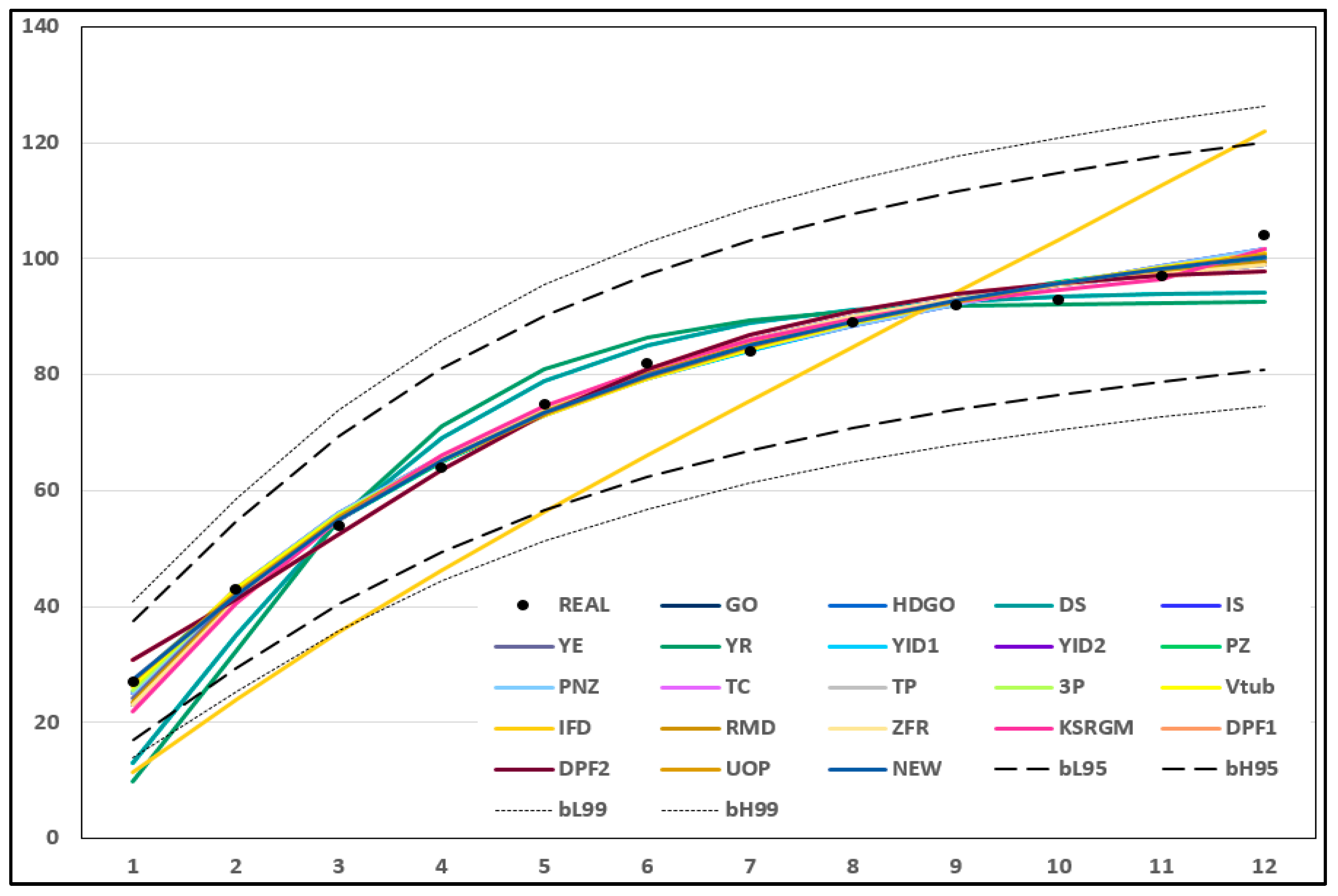
4.3. Results on Dataset 1
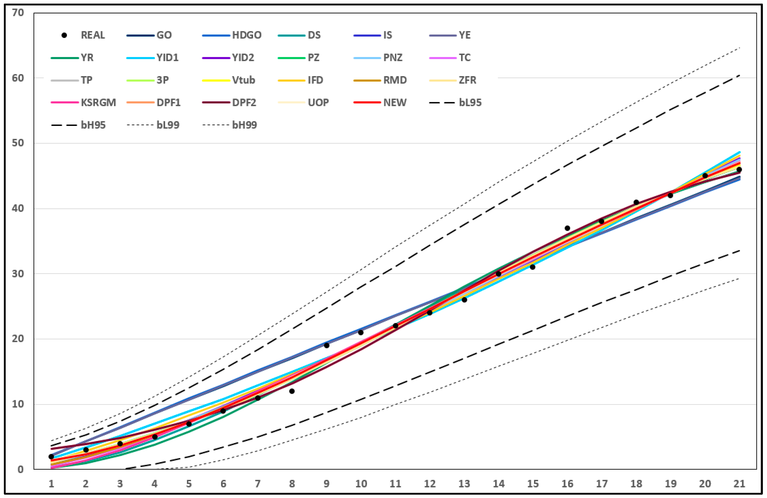
4.4. Results on Dataset 2
5. Conclusions and Remark
Author Contributions
Funding
Data Availability Statement
Acknowledgments
Conflicts of Interest
References
- Goel, A.L.; Okumoto, K. Time-Dependent Error-Detection Rate Model for Software Reliability and Other Performance Measures. IEEE Trans. Reliab. 1979, R-28, 206–211. [Google Scholar] [CrossRef]
- Hossain, S.A.; Dahiya, R.C. Estimating the Parameters of a Non-Homogeneous Poisson-Process Model for Software Reliability. IEEE Trans. Reliab. 1993, 42, 604–612. [Google Scholar] [CrossRef]
- Yamada, S.; Ohba, M.; Osaki, S. S-Shaped Reliability Growth Modeling for Software Error Detection. IEEE Trans. Reliab. 1983, R-32, 475–484. [Google Scholar] [CrossRef]
- Osaki, S.; Hatoyama, Y. Inflexion S-Shaped Software Reliability Growth Models. In Stochastic Models in Reliability Theory; Springer: Berlin/Heidelberg, Germany, 1984; pp. 144–162. [Google Scholar]
- Zhang, X.; Teng, X.; Pham, H. Considering Fault Removal Efficiency in Software Reliability Assessment. IEEE Trans. Syst. Man Cybern.-Part A Syst. Hum. 2003, 33, 114–120. [Google Scholar] [CrossRef]
- Yamada, S.; Ohtera, H.; Narihisa, H. Software Reliability Growth Models with Testing-Effort. IEEE Trans. Reliab. 1986, 35, 19–23. [Google Scholar] [CrossRef]
- Yamada, S.; Tokuno, K.; Osaki, S. Imperfect Debugging Models with Fault Introduction Rate for Software Reliability Assessment. Int. J. Syst. Sci. 1992, 23, 2241–2252. [Google Scholar] [CrossRef]
- Pham, H.; Zhang, X. An NHPP Software Reliability Model and Its Comparison. Int. J. Reliab. Qual. Saf. Eng. 1997, 04, 269–282. [Google Scholar] [CrossRef]
- Pham, H.; Nordmann, L.; Zhang, Z. A General Imperfect-Software-Debugging Model with S-Shaped Fault-Detection Rate. IEEE Trans. Reliab. 1999, 48, 169–175. [Google Scholar] [CrossRef]
- Kapur, P.K.; Pham, H.; Anand, S.; Yadav, K. A Unified Approach for Developing Software Reliability Growth Models in the Presence of Imperfect Debugging and Error Generation. IEEE Trans. Reliab. 2011, 60, 331–340. [Google Scholar] [CrossRef]
- Pham, H. System Software Reliability; Springer: London, UK, 2006. [Google Scholar]
- Roy, P.; Mahapatra, G.S.; Dey, K.N. An NHPP Software Reliability Growth Model with Imperfect Debugging and Error Generation. Int. J. Reliab. Qual. Saf. Eng. 2014, 21, 1450008. [Google Scholar] [CrossRef]
- Li, Q.; Pham, H. Modeling Software Fault-Detection and Fault-Correction Processes by Considering the Dependencies between Fault Amounts. Appl. Sci. 2021, 11, 6998. [Google Scholar] [CrossRef]
- Pan, Z.; Nonaka, Y. Importance Analysis for the Systems with Common Cause Failures. Reliab. Eng. Syst. Saf. 1995, 50, 297–300. [Google Scholar] [CrossRef]
- Kim, Y.S.; Song, K.Y.; Pham, H.; Chang, I.H. A Software Reliability Model with Dependent Failure and Optimal Release Time. Symmetry 2022, 14, 343. [Google Scholar] [CrossRef]
- Lee, D.H.; Chang, I.H.; Pham, H. Software Reliability Model with Dependent Failures and SPRT. Mathematics 2020, 8, 1366. [Google Scholar] [CrossRef]
- Pradhan, V.; Dhar, J.; Kumar, A. Testing Coverage-based Software Reliability Growth Model Considering Uncertainty of Operating Environment. Syst. Eng. 2023, 26, 449–462. [Google Scholar] [CrossRef]
- Teng, X.; Pham, H. A New Methodology for Predicting Software Reliability in the Random Field Environments. IEEE Trans. Reliab. 2006, 55, 458–468. [Google Scholar] [CrossRef]
- Pham, H. A New Software Reliability Model with Vtub-Shaped Fault-Detection Rate and the Uncertainty of Operating Environments. Optimization 2014, 63, 1481–1490. [Google Scholar] [CrossRef]
- Song, K.Y.; Chang, I.H.; Pham, H. A Three-Parameter Fault-Detection Software Reliability Model with the Uncertainty of Operating Environments. J. Syst. Sci. Syst. Eng. 2017, 26, 121–132. [Google Scholar] [CrossRef]
- Haque, M.A.; Ahmad, N. Software Reliability Modeling under an Uncertain Testing Environment. Int. J. Model. Simul. 2023, 1–7. [Google Scholar] [CrossRef]
- Cao, P.; Tang, G.; Zhang, Y.; Luo, Z. Qualitative Evaluation of Software Reliability Considering Many Uncertain Factors. In Ecosystem Assessment and Fuzzy Systems Management; Springer: Cham, Switzerland, 2014; pp. 199–205. [Google Scholar]
- Pachauri, B.; Jain, A.; Raman, S. An Improved SRGM Considering Uncertain Operating Environment. Palest. J. Math. 2022, 11, 38–45. [Google Scholar]
- Asraful Haque, M.; Ahmad, N. A Logistic Growth Model for Software Reliability Estimation Considering Uncertain Factors. Int. J. Reliab. Qual. Saf. Eng. 2021, 28, 2150032. [Google Scholar] [CrossRef]
- Chang, I.H.; Pham, H.; Lee, S.W.; Song, K.Y. A Testing-Coverage Software Reliability Model with the Uncertainty of Operating Environments. Int. J. Syst. Sci. Oper. Logist. 2014, 1, 220–227. [Google Scholar] [CrossRef]
- Lee, D.; Chang, I.; Pham, H. Study of a New Software Reliability Growth Model under Uncertain Operating Environments and Dependent Failures. Mathematics 2023, 11, 3810. [Google Scholar] [CrossRef]
- Singh, P. A Neutrosophic-Entropy Based Adaptive Thresholding Segmentation Algorithm: A Special Application in MR Images of Parkinson’s Disease. Artif. Intell. Med. 2020, 104, 101838. [Google Scholar] [CrossRef] [PubMed]
- Saxena, P.; Kumar, V.; Ram, M. A Novel CRITIC-TOPSIS Approach for Optimal Selection of Software Reliability Growth Model (SRGM). Qual. Reliab. Eng. Int. 2022, 38, 2501–2520. [Google Scholar] [CrossRef]
- Kumar, V.; Saxena, P.; Garg, H. Selection of Optimal Software Reliability Growth Models Using an Integrated Entropy–Technique for Order Preference by Similarity to an Ideal Solution (TOPSIS) Approach. Math. Methods Appl. Sci. 2021, 1–21. [Google Scholar] [CrossRef]
- Garg, R.; Raheja, S.; Garg, R.K. Decision Support System for Optimal Selection of Software Reliability Growth Models Using a Hybrid Approach. IEEE Trans. Reliab. 2022, 71, 149–161. [Google Scholar] [CrossRef]
- Musa, J.D. Software Reliability Data, Deposited in IEEE Computer Society Repository; IEEE: New York, NY, USA, 1979. [Google Scholar]
- Ohba, M. Software Reliability Analysis Models. IBM J. Res. Dev. 1984, 28, 428–443. [Google Scholar] [CrossRef]
- Armstrong, J.S.; Collopy, F. Error Measures for Generalizing about Forecasting Methods: Empirical Comparisons. Int. J. Forecast. 1992, 8, 69–80. [Google Scholar] [CrossRef]
- Piper, E.L.; Boote, K.J.; Jones, J.W.; Grimm, S.S. Comparison of Two Phenology Models for Predicting Flowering and Maturity Date of Soybean. Crop Sci. 1996, 36, 1606–1614. [Google Scholar] [CrossRef]
- Iqbal, J. Software Reliability Growth Models: A Comparison of Linear and Exponential Fault Content Functions for Study of Imperfect Debugging Situations. Cogent Eng. 2017, 4, 1286739. [Google Scholar] [CrossRef]
- Akossou, A.Y.J.; Palm, R. Impact of Data Structure on the Estimators R-Square and Adjusted R-Square in Linear Regression. Int. J. Math. Comput. 2013, 20, 84–93. [Google Scholar]
- Sharma, K.; Garg, R.; Nagpal, C.K.; Garg, R.K. Selection of Optimal Software Reliability Growth Models Using a Distance Based Approach. IEEE Trans. Reliab. 2010, 59, 266–276. [Google Scholar] [CrossRef]
- Willmott, C.; Matsuura, K. Advantages of the Mean Absolute Error (MAE) over the Root Mean Square Error (RMSE) in Assessing Average Model Performance. Clim. Res. 2005, 30, 79–82. [Google Scholar] [CrossRef]
- Kuha, J. AIC and BIC. Sociol. Methods Res. 2004, 33, 188–229. [Google Scholar] [CrossRef]
- Weakliem, D.L. A Critique of the Bayesian Information Criterion for Model Selection. Sociol. Methods Res. 1999, 27, 359–397. [Google Scholar] [CrossRef]
- Xu, J.; Yao, S. Software Reliability Growth Model with Partial Differential Equation for Various Debugging Processes. Math. Probl. Eng. 2016, 2016, 2476584. [Google Scholar] [CrossRef]
- Witt, S.F.; Witt, C.A. Modeling and Forecasting Demand in Tourism; Academic Press: London, UK, 1992. [Google Scholar]
- Allen, D.M. Mean Square Error of Prediction as a Criterion for Selecting Variables. Technometrics 1971, 13, 469–475. [Google Scholar] [CrossRef]
- Ali, N.N. A Comparison of Some Information Criteria to Select a Weather Forecast Model. Turk. J. Comput. Math. Educ. (TURCOMAT) 2021, 12, 2494–2500. [Google Scholar]
- Pham, H. On Estimating the Number of Deaths Related to COVID-19. Mathematics 2020, 8, 655. [Google Scholar] [CrossRef]
- Wang, L.; Hu, Q.; Liu, J. Software Reliability Growth Modeling and Analysis with Dual Fault Detection and Correction Processes. IIE Trans. 2016, 48, 359–370. [Google Scholar] [CrossRef]
- Gamiz, M.L.; Navas-Gomez, F.J.; Raya-Miranda, R. A Machine Learning Algorithm for Reliability Analysis. IEEE Trans. Reliab. 2021, 70, 535–546. [Google Scholar] [CrossRef]
- Kumar, P.; Singh, Y. An Empirical Study of Software Reliability Prediction Using Machine Learning Techniques. Int. J. Syst. Assur. Eng. Manag. 2012, 3, 194–208. [Google Scholar] [CrossRef]
- Jaiswal, A.; Malhotra, R. Software Reliability Prediction Using Machine Learning Techniques. Int. J. Syst. Assur. Eng. Manag. 2018, 9, 230–244. [Google Scholar] [CrossRef]
- Wang, J.; Zhang, C. Software Reliability Prediction Using a Deep Learning Model Based on the RNN Encoder–Decoder. Reliab. Eng. Syst. Saf. 2018, 170, 73–82. [Google Scholar] [CrossRef]
- Li, C.; Zheng, J.; Okamura, H.; Dohi, T. Software Reliability Prediction through Encoder-Decoder Recurrent Neural Networks. Int. J. Math. Eng. Manag. Sci. 2022, 7, 325–340. [Google Scholar] [CrossRef]
- Zainuddin, Z.; EA, P.A.; Hasan, M.H. Predicting Machine Failure Using Recurrent Neural Network-Gated Recurrent Unit (RNN-GRU) through Time Series Data. Bull. Electr. Eng. Inform. 2021, 10, 870–878. [Google Scholar]
- Wang, H.; Zhuang, W.; Zhang, X. Software Defect Prediction Based on Gated Hierarchical LSTMs. IEEE Trans. Reliab. 2021, 70, 711–727. [Google Scholar] [CrossRef]

| No. | Model | Mean Value Function | Note |
|---|---|---|---|
| 1 | Goel-Okumoto (GO) [1] | Concave | |
| 2 | Hossain-Dahiya (HDGO) [2] | Concave | |
| 3 | Yamada et al. (DS) [3] | S-Shape | |
| 4 | Ohba (IS) [4] | S-Shape | |
| 5 | Yamada et al. (YE) [6] | Concave | |
| 6 | Yamada et al. (YR) [6] | S-Shape | |
| 7 | Yamada et al. (YID 1) [7] | Concave | |
| 8 | Yamada et al. (YID 2) [7] | Concave | |
| 9 | Pham-Zhang (PZ) [8] | Both | |
| 10 | Pham et al. (PNZ) [9] | Both | |
| 11 | Pham (IFD) [11] | Concave | |
| 12 | Roy et al. (RMD) [12] | Concave | |
| 13 | Zhang et al. (ZFR) [5] | S-Shape | |
| 14 | Kapur et al. (KSRGM) [10] | S-Shape | |
| 15 | Chang et al. (TC) [25] | Both | |
| 16 | Teng-Pham (TP) [18] | S-Shape | |
| 17 | Song et al. (3P) [20] | S-Shape | |
| 18 | Pham (Vtub) [19] | S-Shape | |
| 19 | Kim et al. (DPF1) [15] | Concave, Dependent | |
| 20 | Lee et al. (DPF2) [16] | Concave, Dependent | |
| 21 | Lee et al. (UOP) [26] | S-Shape, Dependent | |
| 22 | Proposed Model | S-Shape |
| No. | Criteria | Formula |
|---|---|---|
| 1 | MSE | |
| 2 | RMSE | |
| 3 | PRR | |
| 4 | PP | |
| 5 | ||
| 6 | ||
| 7 | MAE | |
| 8 | AIC | |
| 9 | BIC | |
| 10 | PRV | |
| 11 | RMSPE | |
| 12 | MEOP | |
| 13 | TS | |
| 14 | PIC | |
| 15 | PC |
| No | Model | |||||||||||
|---|---|---|---|---|---|---|---|---|---|---|---|---|
| 1 | GO | 103.9957 | 0.25072 | |||||||||
| 2 | HDGO | 103.9956 | 0.25072 | 0.003999 | ||||||||
| 3 | DS | 94.42989 | 0.64986 | |||||||||
| 4 | IS | 103.9919 | 0.250789 | 0.000336 | ||||||||
| 5 | YE | 135.4096 | 0.079955 | 0.118615 | 22.03046 | |||||||
| 6 | YR | 99.87051 | 0.30301 | 0.081458 | 8.609839 | |||||||
| 7 | YID1 | 80.07877 | 0.368316 | 0.026422 | ||||||||
| 8 | YID2 | 77.60045 | 0.381731 | 0.033943 | ||||||||
| 9 | PZ | 94.9835 | 4.728741 | 0.203146 | 3.469121 | 13.93669 | ||||||
| 10 | PNZ | 77.57743 | 0.382112 | 0.033973 | 0.000898 | |||||||
| 11 | IFD | 11.11251 | 0.830547 | 1.07 × 10−0.7 | ||||||||
| 12 | RMD | 20.84912 | 0.289209 | 5.46394 | 0.069861 | |||||||
| 13 | ZFR | 16.75903 | 0.009765 | 0.010496 | 0.158331 | 1.571965 | 0.319499 | |||||
| 14 | KSRGM | 50.34612 | 67.63962 | 0.504539 | 0.008162 | |||||||
| 15 | TC | 0.123963 | 0.887039 | 2.764066 | 1.760686 | 125.3202 | ||||||
| 16 | TP | 273.867 | 0.001876 | 78.32247 | 0.094677 | 15.26608 | 3.2414 | 0.611472 | ||||
| 17 | 3P | 7.009842 | 5.44 × 10⁻⁸ | 0.131806 | 137.9787 | 234.0264 | ||||||
| 18 | Vtub | 1.050673 | 0.921887 | 1.257807 | 0.251814 | 127.3638 | ||||||
| 19 | DPF1 | 99.2143 | 0.00489 | 0.060524 | 28.30202 | |||||||
| 20 | DPF2 | 99.21582 | 0.000271 | 0.058441 | 28.30183 | |||||||
| 21 | UOP | 0.959106 | 0.248168 | 1.021567 | 0.927368 | 133.764 | ||||||
| 22 | NEW | 2.750654 | 1.406831 | 127.7906 |
| Criteria | GO | HDGO | DS | IS | YE | YR | YID1 | YID2 | PZ | PNZ | IFD |
|---|---|---|---|---|---|---|---|---|---|---|---|
| MSE | 6.474 | 7.193 | 44.306 | 7.196 | 5.728 | 87.848 | 3.994 | 4.040 | 5.413 | 4.546 | 291.502 |
| RMSE | 2.544 | 2.682 | 6.656 | 2.683 | 2.393 | 9.373 | 1.999 | 2.010 | 2.327 | 2.132 | 17.073 |
| PRR | 0.037 | 0.037 | 1.205 | 0.037 | 0.019 | 3.155 | 0.012 | 0.011 | 0.005 | 0.011 | 3.110 |
| PP | 0.029 | 0.029 | 0.323 | 0.029 | 0.016 | 0.505 | 0.011 | 0.011 | 0.005 | 0.011 | 0.900 |
| R2 | 0.990 | 0.990 | 0.928 | 0.990 | 0.993 | 0.886 | 0.994 | 0.994 | 0.994 | 0.994 | 0.574 |
| adjR2 | 0.987 | 0.986 | 0.912 | 0.986 | 0.988 | 0.821 | 0.992 | 0.992 | 0.989 | 0.991 | 0.414 |
| MAE | 2.274 | 2.526 | 5.566 | 2.526 | 2.510 | 8.872 | 1.948 | 1.963 | 2.396 | 2.210 | 18.217 |
| AIC | 67.156 | 69.156 | 115.306 | 69.160 | 67.385 | 158.805 | 61.394 | 61.667 | 68.850 | 63.665 | 100.809 |
| BIC | 68.126 | 70.610 | 116.275 | 70.614 | 69.325 | 160.745 | 62.848 | 63.121 | 71.275 | 65.605 | 102.264 |
| PRV | 2.412 | 2.412 | 6.230 | 2.412 | 2.036 | 7.823 | 1.807 | 1.817 | 1.856 | 1.817 | 14.116 |
| RMSPE | 2.425 | 2.425 | 6.337 | 2.425 | 2.041 | 7.979 | 1.808 | 1.818 | 1.856 | 1.818 | 15.337 |
| MEOP | 2.067 | 2.274 | 5.060 | 2.274 | 2.231 | 7.886 | 1.753 | 1.766 | 2.097 | 1.965 | 16.395 |
| TS | 2.953 | 2.953 | 7.725 | 2.953 | 2.484 | 9.729 | 2.200 | 2.213 | 2.259 | 2.213 | 18.797 |
| PC | 10.627 | 11.251 | 20.244 | 11.253 | 10.860 | 21.781 | 8.604 | 8.656 | 11.881 | 9.935 | 27.910 |
| PIC | 66.939 | 68.405 | 445.261 | 68.429 | 51.327 | 708.287 | 39.612 | 40.030 | 45.746 | 41.864 | 2627.181 |
| MCDMR | 0.01486 | 0.02002 | 0.10848 | 0.02181 | 0.01322 | 0.18699 | 0.00254 | 0.00414 | 0.01381 | 0.00577 | 0.00904 |
| Criteria | RMD | ZFR | KSRGM | TC | TP | 3P | Vtub | DPF1 | DPF2 | UOP | NEW |
| MSE | 6.760 | 10.797 | 6.542 | 5.166 | 12.833 | 5.352 | 5.192 | 10.760 | 10.760 | 4.798 | 3.834 |
| RMSE | 2.600 | 3.286 | 2.558 | 2.273 | 3.582 | 2.314 | 2.279 | 3.280 | 3.280 | 2.190 | 1.958 |
| PRR | 0.028 | 0.037 | 0.062 | 0.006 | 0.037 | 0.009 | 0.006 | 0.026 | 0.026 | 0.005 | 0.005 |
| PP | 0.023 | 0.029 | 0.043 | 0.006 | 0.029 | 0.009 | 0.006 | 0.030 | 0.030 | 0.005 | 0.005 |
| R2 | 0.991 | 0.990 | 0.992 | 0.994 | 0.990 | 0.994 | 0.994 | 0.986 | 0.986 | 0.995 | 0.994 |
| adjR2 | 0.986 | 0.977 | 0.987 | 0.989 | 0.971 | 0.989 | 0.989 | 0.978 | 0.978 | 0.990 | 0.992 |
| MAE | 2.656 | 3.790 | 2.495 | 2.425 | 4.528 | 2.531 | 2.458 | 3.254 | 3.254 | 2.326 | 1.878 |
| AIC | 68.697 | 75.164 | 61.969 | 67.149 | 77.048 | 67.226 | 66.973 | 81.712 | 81.710 | 67.235 | 63.825 |
| BIC | 70.636 | 78.074 | 63.908 | 69.573 | 80.443 | 69.650 | 69.398 | 83.651 | 83.649 | 69.660 | 65.280 |
| PRV | 2.208 | 2.413 | 2.152 | 1.813 | 2.401 | 1.845 | 1.818 | 2.797 | 2.797 | 1.747 | 1.771 |
| RMSPE | 2.217 | 2.426 | 2.179 | 1.813 | 2.414 | 1.846 | 1.818 | 2.797 | 2.797 | 1.747 | 1.771 |
| MEOP | 2.361 | 3.249 | 2.218 | 2.122 | 3.773 | 2.215 | 2.150 | 2.893 | 2.893 | 2.036 | 1.691 |
| TS | 2.699 | 2.954 | 2.655 | 2.207 | 2.940 | 2.246 | 2.212 | 3.405 | 3.405 | 2.127 | 2.156 |
| PC | 11.522 | 16.058 | 11.391 | 11.718 | 19.591 | 11.842 | 11.736 | 13.382 | 13.381 | 11.459 | 8.420 |
| PIC | 59.581 | 75.779 | 57.836 | 44.021 | 79.566 | 45.323 | 44.203 | 91.581 | 91.579 | 41.444 | 38.176 |
| MCDMR | 0.03436 | 0.01289 | 0.00987 | 0.39357 | 0.01903 | 0.03164 | 0.01472 | 0.03334 | 0.03262 | 0.00745 | 0.00253 |
| No | Model | |||||||||||
|---|---|---|---|---|---|---|---|---|---|---|---|---|
| 1 | GO | 258479.7 | 8.27 × 10−0.6 | |||||||||
| 2 | HDGO | 709.7827 | 0.003083 | 0.462394 | ||||||||
| 3 | DS | 77.25299 | 0.096622 | |||||||||
| 4 | IS | 59.28546 | 0.16839 | 8.278172 | ||||||||
| 5 | YE | 4709.105 | 2.411867 | 0.000372 | 0.507832 | |||||||
| 6 | YR | 77.83392 | 2.677162 | 0.004541 | 0.522922 | |||||||
| 7 | YID1 | 19614.07 | 8.39 × 10−0.5 | 0.030908 | ||||||||
| 8 | YID2 | 1.491036 | 0.306843 | 1.745694 | ||||||||
| 9 | PZ | 17.01691 | 0.153619 | 0.16534 | 5.82304 | 44.56855 | ||||||
| 10 | PNZ | 11.71105 | 0.195293 | 0.198144 | 1.382584 | |||||||
| 11 | IFD | 8.684959 | 0.138925 | 0.023631 | ||||||||
| 12 | RMD | 104.218 | 0.033806 | 1.146429 | 0.149771 | |||||||
| 13 | ZFR | 38.40169 | 0.193953 | 5.65856 | 0.17475 | 0.178089 | 0.753317 | |||||
| 14 | KSRGM | 32.74804 | 0.98946 | 0.821748 | 0.108743 | |||||||
| 15 | TC | 0.019064 | 1.567033 | 839.154 | 221.1735 | 78.78594 | ||||||
| 16 | TP | 102.844 | 0.173628 | 1.206102 | 1.133787 | 16.86387 | 1.556427 | 0.089124 | ||||
| 17 | 3P | 0.49233 | 0.168722 | 0.240659 | 61.55869 | 116.1341 | ||||||
| 18 | Vtub | 1.970059 | 0.689159 | 0.292767 | 19.85291 | 87.25193 | ||||||
| 19 | DPF1 | 51.44718 | 0.004767 | 0.028006 | 2.634778 | |||||||
| 20 | DPF2 | 51.45985 | 5.03 × 10⁻⁵ | 0.010786 | 2.633591 | |||||||
| 21 | UOP | 0.467491 | 0.042319 | 1.537043 | 1.497623 | 226.1843 | ||||||
| 22 | NEW | 33.62065 | 4.901007 | 167.9314 |
| Criteria | GO | HDGO | DS | IS | YE | YR | YID1 | YID2 | PZ | PNZ | IFD |
|---|---|---|---|---|---|---|---|---|---|---|---|
| MSE | 6.568 | 7.728 | 1.637 | 1.395 | 7.559 | 2.420 | 2.936 | 1.701 | 1.564 | 1.646 | 2.104 |
| RMSE | 2.563 | 2.780 | 1.279 | 1.181 | 2.749 | 1.556 | 1.714 | 1.304 | 1.251 | 1.283 | 1.451 |
| PRR | 0.805 | 0.863 | 26.321 | 0.679 | 0.817 | 55.688 | 0.356 | 3.064 | 0.843 | 0.968 | 0.451 |
| PP | 1.852 | 2.041 | 1.208 | 0.297 | 1.889 | 1.588 | 0.526 | 0.608 | 0.331 | 0.369 | 0.351 |
| R2 | 0.972 | 0.969 | 0.993 | 0.994 | 0.972 | 0.991 | 0.988 | 0.993 | 0.994 | 0.994 | 0.992 |
| adjR2 | 0.969 | 0.964 | 0.992 | 0.993 | 0.964 | 0.989 | 0.986 | 0.992 | 0.993 | 0.992 | 0.990 |
| MAE | 2.232 | 2.525 | 1.107 | 0.973 | 2.545 | 1.477 | 1.542 | 1.170 | 1.104 | 1.157 | 1.305 |
| AIC | 77.325 | 79.554 | 78.118 | 76.699 | 81.386 | 83.031 | 79.127 | 78.662 | 80.793 | 79.560 | 78.284 |
| BIC | 79.414 | 82.688 | 80.207 | 79.832 | 85.564 | 87.209 | 82.261 | 81.796 | 86.016 | 83.738 | 81.417 |
| PRV | 2.325 | 2.459 | 1.224 | 1.120 | 2.371 | 1.375 | 1.606 | 1.236 | 1.118 | 1.183 | 1.372 |
| RMSPE | 2.490 | 2.629 | 1.246 | 1.120 | 2.527 | 1.432 | 1.625 | 1.237 | 1.119 | 1.183 | 1.376 |
| MEOP | 2.120 | 2.392 | 1.052 | 0.921 | 2.403 | 1.395 | 1.461 | 1.109 | 1.039 | 1.093 | 1.236 |
| TS | 9.047 | 9.552 | 4.516 | 4.058 | 9.181 | 5.195 | 5.887 | 4.481 | 4.052 | 4.284 | 4.984 |
| PC | 19.035 | 20.350 | 5.834 | 4.940 | 20.103 | 10.423 | 11.639 | 6.726 | 7.655 | 7.146 | 8.642 |
| PIC | 126.890 | 142.437 | 33.200 | 28.438 | 133.214 | 45.851 | 56.180 | 33.948 | 31.280 | 32.690 | 41.213 |
| MCDMR | 0.09265 | 0.11500 | 0.03568 | 0.00512 | 0.10967 | 0.08481 | 0.04813 | 0.02263 | 0.01316 | 0.01963 | 0.03299 |
| Criteria | RMD | ZFR | KSRGM | TC | TP | 3P | Vtub | DPF1 | DPF2 | UOP | NEW |
| MSE | 1.616 | 1.671 | 1.850 | 1.723 | 1.794 | 1.569 | 1.544 | 2.002 | 2.001 | 1.573 | 1.387 |
| RMSE | 1.271 | 1.293 | 1.360 | 1.313 | 1.339 | 1.253 | 1.243 | 1.415 | 1.415 | 1.254 | 1.178 |
| PRR | 3.112 | 0.797 | 36.310 | 6.012 | 0.707 | 0.681 | 0.561 | 0.336 | 0.336 | 0.271 | 0.375 |
| PP | 0.611 | 0.321 | 1.174 | 0.760 | 0.303 | 0.297 | 0.270 | 0.583 | 0.582 | 0.193 | 0.231 |
| R2 | 0.994 | 0.994 | 0.993 | 0.994 | 0.994 | 0.994 | 0.995 | 0.992 | 0.992 | 0.994 | 0.995 |
| adjR2 | 0.992 | 0.992 | 0.991 | 0.992 | 0.991 | 0.993 | 0.993 | 0.991 | 0.991 | 0.993 | 0.994 |
| MAE | 1.150 | 1.179 | 1.239 | 1.207 | 1.257 | 1.095 | 1.094 | 1.204 | 1.203 | 1.131 | 0.998 |
| AIC | 80.090 | 82.790 | 83.337 | 82.566 | 84.738 | 80.702 | 80.602 | 78.795 | 78.792 | 80.563 | 76.587 |
| BIC | 84.268 | 89.057 | 87.515 | 87.788 | 92.049 | 85.924 | 85.824 | 82.973 | 82.970 | 85.786 | 79.720 |
| PRV | 1.170 | 1.119 | 1.245 | 1.169 | 1.120 | 1.120 | 1.110 | 1.300 | 1.300 | 1.122 | 1.117 |
| RMSPE | 1.172 | 1.119 | 1.254 | 1.174 | 1.121 | 1.120 | 1.111 | 1.304 | 1.304 | 1.122 | 1.117 |
| MEOP | 1.086 | 1.105 | 1.170 | 1.136 | 1.173 | 1.030 | 1.030 | 1.137 | 1.136 | 1.065 | 0.946 |
| TS | 4.244 | 4.054 | 4.542 | 4.252 | 4.059 | 4.058 | 4.025 | 4.725 | 4.723 | 4.063 | 4.047 |
| PC | 6.987 | 9.326 | 8.140 | 8.425 | 11.252 | 7.679 | 7.549 | 8.810 | 8.805 | 7.700 | 4.891 |
| PIC | 32.171 | 33.061 | 36.160 | 33.810 | 35.114 | 31.356 | 30.952 | 38.740 | 38.719 | 31.423 | 28.301 |
| MCDMR | 0.01999 | 0.02143 | 0.05685 | 0.03090 | 0.02850 | 0.01373 | 0.00941 | 0.03148 | 0.02953 | 0.01523 | 0.00271 |
Disclaimer/Publisher’s Note: The statements, opinions and data contained in all publications are solely those of the individual author(s) and contributor(s) and not of MDPI and/or the editor(s). MDPI and/or the editor(s) disclaim responsibility for any injury to people or property resulting from any ideas, methods, instructions or products referred to in the content. |
© 2024 by the authors. Licensee MDPI, Basel, Switzerland. This article is an open access article distributed under the terms and conditions of the Creative Commons Attribution (CC BY) license (https://creativecommons.org/licenses/by/4.0/).
Share and Cite
Song, K.Y.; Kim, Y.S.; Pham, H.; Chang, I.H. A Software Reliability Model Considering a Scale Parameter of the Uncertainty and a New Criterion. Mathematics 2024, 12, 1641. https://doi.org/10.3390/math12111641
Song KY, Kim YS, Pham H, Chang IH. A Software Reliability Model Considering a Scale Parameter of the Uncertainty and a New Criterion. Mathematics. 2024; 12(11):1641. https://doi.org/10.3390/math12111641
Chicago/Turabian StyleSong, Kwang Yoon, Youn Su Kim, Hoang Pham, and In Hong Chang. 2024. "A Software Reliability Model Considering a Scale Parameter of the Uncertainty and a New Criterion" Mathematics 12, no. 11: 1641. https://doi.org/10.3390/math12111641
APA StyleSong, K. Y., Kim, Y. S., Pham, H., & Chang, I. H. (2024). A Software Reliability Model Considering a Scale Parameter of the Uncertainty and a New Criterion. Mathematics, 12(11), 1641. https://doi.org/10.3390/math12111641