Abstract
The Gegenbauer autoregressive moving-average (GARMA) model is pivotal for addressing non-additivity, non-normality, and heteroscedasticity in real-world time-series data. While primarily recognized for its efficacy in various domains, including the health sector for forecasting COVID-19 cases, this study aims to assess its performance using yearly sunspot data. We evaluate the GARMA model’s goodness of fit and parameter estimation specifically within the domain of sunspots. To achieve this, we introduce the random coefficient generalized autoregressive moving-average (RCGARMA) model and develop methodologies utilizing conditional least squares (CLS) and conditional weighted least squares (CWLS) estimators. Employing the ratio of mean squared errors (RMSE) criterion, we compare the efficiency of these methods using simulation data. Notably, our findings highlight the superiority of the conditional weighted least squares method over the conditional least squares method. Finally, we provide an illustrative application using two real data examples, emphasizing the significance of the GARMA model in sunspot research.
Keywords:
GARMA model; conditional least squares; weighted conditional least squares; mean squared errors MSC:
62M10; 62F10; 62F12
1. Introduction
Fitting a Gegenbauer autoregressive moving-average (GARMA) model to non-Gaussian data becomes intricate when real-world time series exhibit high anomalies, such as non-additivity and heteroscedasticity. Addressing this behavior has garnered significant interest, leading to numerous studies over the past few decades. For example, Albarracin et al. [1] analyzed the structure of GARMA models in practical applications, Huntet al. [2] proposed an R (Version R-4.4.0) package called ’garma’ to fit and forecast GARMA models, and Darmawan et al. [3] used a GARMA model to forecast COVID-19 data in Indonesia.
The conditional heteroscedastic autoregressive moving-average (CHARMA) model is commonly employed to capture unobserved heterogeneity characteristics in real-world data [4]. Another closely related model is the random coefficient autoregressive (RCA) model, introduced by Nicholls and Quinn [5], with recent investigations into its properties conducted by Appadoo et al [6].
The GARMA model has recently emerged as a suitable framework to identify and handle such features in real-world data under specific parameter values [7]. An inference for the estimators of the GARMA model was given by Beaumont and Smallwood [8], and an efficient estimation approach for the regression parameters of the generalized autoregressive moving-average model was provided by Hossain et al. [9].
In this context, this study proposes a random coefficient approach, namely the random coefficient Gegenbauer autoregressive moving-average (RCGARMA) model, to capture unobserved heterogeneity. The RCGARMA model extends the GARMA model by introducing an additional source of random variation to the standard coefficient model. While the GARMA model has been extensively analyzed with non-random coefficients (see [10,11,12], among others), the RCGARMA model provides flexibility in modeling unobserved heterogeneity in profit structures of dependent data, alongside long short-term dependence and seasonal fluctuations at different frequencies. Analyzing the statistical properties and estimation of this model is crucial for its application to real-world data.
To begin, we introduce the fundamentals of the random GARMA model, along with notations and commonly used assumptions. Throughout this paper, we focus on random coefficients in the GARMA model, akin to random-effect regression models, where the fixed coefficients of the GARMA model are randomly perturbed (see, for example, [13,14], and other relevant literature).
We consider a scenario in which we observe a sequence of random variables , generated by the following recursive model [15]:
where is the noise, which is assumed to have zero mean and variance , and is determined by the following assumptions:
where are the Gegenbauer polynomial coefficients, defined in terms of their generating function (see, for instance, Magnus et al. [16] and Rainville and Earl [17]), as follows:
where denotes the Gamma function and stands for the integer part of [2].
Therefore, in this study, we extend the GARMA models to RCGARMA models, as discussed above, by including dynamic random coefficient effects. We assume that the row vector of coefficients, in Equation (2), that gives the impact of the time-varying variables on in Equation (1), initially presumed to be fixed and time-invariant parameters, does change over time. In this scenario, the parameter vector can be partitioned as , where is constant reflecting the fixed coefficients, and denotes the sequence of random coefficients related to the nuisance parameters that can be omitted from the model. To identify this model, we assume that and . It is also assumed that is uncorrelated with , and that for all t and s. We use to represent the set of all model coefficients, then the general model (Equation (1)) becomes:
The concept of fixed and random coefficient time-series models has been applied for testing the presence of random coefficients in autoregressive models [18], and for handling the possible nonlinear features of real-world data [19]. Another relevant reference is the study by Mundlak [20], which introduced the dynamic random effects model for panel data analysis. Mundlak’s work highlights the importance of incorporating time-varying random effects into panel data.
In this context, it can be implicitly assumed that truncating the right-hand side of Equation (3) at lag m is valid for n = 0, 1, …, m. Under this assumption, the RCGARMA model should be accurately formulated as follows:
where the sequence represents the truncated Gegenbauer process, with its behavior contingent on the selected finite truncation lag order denoted by …. This concept draws parallels to the MA approximation presented by Dissanayake et al. [21], along with comprehensive literature reviews on diverse issues in long-memory time series, encompassing Gegenbauer processes and their associated properties. … is an vector of random coefficients. … is an vector of past observations.
Concerning the estimation of the unknown parameters of interest, we define a vector denoted as . Under the assumption that the random sequences are allowed to exhibit correlations with the error process , we represent
where is the matrix representing the variance of , is the vector representing the covariance between and , and is the variance of the error process .
The ordinary least squares (OLS) method is commonly used in this case. This method aims to estimate the parameters by minimizing the sum of squared differences between the observed and predicted values, and it assumes the independence, homoskedasticity, and normality of error distribution.
However, the assumptions of our model do not align with those of ordinary least squares estimation. While OLS assumes independence and homoskedasticity of errors, our model may exhibit heteroskedasticity and correlation structures due to the presence of random effects. Additionally, the errors in our model are not strictly bound to a normal distribution.
To address these issues, we employ an estimation procedure using conditional least squares (CLS) and weighted least squares (WLS) estimators. CLS adjusts for heteroskedasticity by incorporating the conditional variance structure into the estimation process, while WLS provides more robust estimates compared to OLS by assigning weights to observations based on their variances. This methodology is based on the work proposed by Hwang and Basawa [22], which has demonstrated favorable performance for generalized random coefficient autoregressive processes. Additionally, the studies by Nicholls and Quinn [5] and Hwang and Basawa [23] are also relevant in this context.
By implementing these procedures, one can obtain significant estimates for random effects. This paper begins by assessing the parameters using the conditional least squares estimation method in Section 2. Section 3 introduces an alternative estimator based on the weighted conditional least squares estimation method. Following this, Section 4 and Section 5 compare the performance of these methods using simulation data and real-world data, respectively.
2. Conditional Least Squares Estimation Method
The conditional least squares estimation method is a flexible technique commonly used for estimation. It offers valuable characteristics like consistency and asymptotic normality under specific conditions. This approach is valuable because it helps ensure that the estimated coefficients approach the true values as more data are obtained, which is known as consistency. Furthermore, the asymptotic normality property indicates that as the sample size increases, the distribution of the estimators approximates a normal distribution. By minimizing the sum of squared deviations, we are essentially finding the best-fitting line or curve that represents the relationship between variables in the data, making it a widely used and reliable technique in statistical analysis.
The utilization of conditional least squares estimation in the context of GARMA models with random effects provides a robust approach to estimating model parameters while accounting for the inherent uncertainties and complexities introduced by random effects. Conditional least squares estimation in random effects GARMA models stands out for its capability to handle issues stemming from unobserved heterogeneity and time-varying dynamics [24]. This approach enables researchers to discern the influence of random effects on model parameters, thereby enhancing the interpretability and robustness of the estimated coefficients [25].
Moreover, the interpretability of the results obtained through CLS estimation in GARMA models with random effects is augmented by the incorporation of a conditional framework. By conditioning the estimation on information present at each time point, researchers can acquire a deeper understanding of the temporal progression of model parameters and their individual impacts on the observed data [26].
In this section, we use the conditional least squares method to estimate the unknown parameters in the RCGARMA model. Viewing it as a regression model with the predictor variable and response variable , the least squares estimation involves minimizing the sum of squares of the differences. The initial step involves estimating the vector mean parameters of the regression function (see Equation (4)).
2.1. Estimation of Parameters
In this section, we discuss the estimation of through the utilization of the conditional least squares estimation procedure. The estimator, denoted as , represents the optimal selection of values for our parameters and is calculated using a sample (……). When performing conditional least squares estimation, the objective is to minimize the following conditional sum of squares:
with respect to the vector …. This is achieved by solving the system .
Replacing in the last equation with yields the following result:
The derivation of the asymptotic properties of our estimator relies on the following standard conditions:
- (C.0)
- The square matrix must have full rank.
- (C.1)
- The stationary distribution of must have a fourth-order moment, meaning that .
In time-series analysis, condition (C.0) is crucial for the estimation process. It requires the square matrix to have full rank. This condition essentially ensures that the information provided by the data is sufficient and not redundant, allowing for accurate estimation of the parameters. When this condition is met, it facilitates reliable inference and prediction based on the time-series data. The condition in the time series, identified as (C.1), states that the stationary distribution of needs to exhibit a fourth-order moment, indicating that . Now, assuming that these two conditions are verified, we have the following theorem, which describes the limit distribution of the estimator of .
Theorem 1.
Let be the estimator of Θ. Under (C.0) and (C.1), we have:
where
and
with
Proof.
To prove the result of this theorem, let
Let …, where , j = 1, …, m. Consider
where
Given that is a stationary ergodic zero-mean martingale difference for all t = 1, …, m, we apply the central limit theorem for stationary ergodic martingale differences proposed by Billingsley [27].
Thus, we find that
Furthermore, by the ergodic theorem, we have
□
Therefore, the result of Theorem 1 is proven.
In the following section, we calculate the estimators for the variance component parameters of the RCGARMA model described earlier. These parameters define the variance of random errors, the covariances between errors and random effects, and the variance matrix parameters of random effects in the model. The covariance matrix is typically expressed as a mysterious linear combination of known cofactor matrices, as shown below.
2.2. Covariance Parameter Estimators
Let be the unknown parameter vector containing all model parameters representing the variance components. We partition the parameter vector into three sub-vectors: includes all parameters related to the time-invariant variance of errors, includes all covariance parameters in the RCGARMA process, and includes parameters for the matrix elements of the variance of random effects in the RCGARMA process. Specifically, it can be noted as:
where and denotes the (i,j)th element of the variance matrix of , .
To estimate the variance component parameters in the RCGARMA model using the least squares estimator, assume the available dataset is ……, and note that and in Equation (6) are, respectively, given as follows:
The conditional least squares estimator is used to estimate the parameters . This method allows researchers to decompose the total variability observed in the data into different components, including the variance contributed by random model effects. A study by Ngatchou-Wandji [28] applied conditional least squares to estimate the parameters in a class of heteroscedastic time-series models, demonstrating its consistency and its asymptotic normality.
By utilizing conditional least squares to estimate variance components in the RCGARMA model (e.g., GARMA models with random effects), the estimator, denoted as , is acquired by minimizing the sum of squares represented by . This process allows us to derive the conditional least squares estimator , where is given by Equation (5) for . The estimator is obtained as a solution to the equation represented by:
The derivation of the asymptotic properties of our estimator relies on the following standard conditions: (C.0), as described above, and (C.2), which states that the stationary distribution of must have an eight-order moment, meaning that .
Then, it can be shown that can converge in distribution to a multinormal matrix, as given in the theorem below.
Theorem 2.
Under (C.0) and (C.2), we have:
where
and
Proof.
See [22]. □
3. Weighted Conditional Least Squares Estimation Method
The weighted conditional least squares estimation method for generalized autoregressive moving-average (GARMA) models with random effects is a sophisticated statistical technique used to improve efficiency in the presence of heteroskedasticity. The traditional ordinary least squares estimation used above may not be the optimal choice when dealing with data exhibiting varying error variances, as it does not take this heteroskedasticity into account. In such cases, a more suitable approach involves employing a conditional weighted least squares estimator for the parameter of interest, denoted as . By incorporating weighted factors into the estimation process, this method assigns different weights to observations based on the variability of their error terms.
This allows for a more precise estimation of the parameters in the presence of heteroscedasticity in GARMA models, ultimately leading to more reliable statistical inference. This approach is particularly crucial when faced with heteroskedasticity in the data, as mentioned in in Equation (3).
The recognition of this heteroskedasticity highlights the need for more advanced estimation techniques to ensure the accuracy and reliability of the statistical analysis. This section concentrates on implementing this approach. We seek to enhance efficiency by employing a conditional weighted least squares estimator for .
Assuming that the nuisance parameter is known, the weighted conditional least squares estimator of is obtained by minimizing:
Since and , the estimator is given by:
Consider the following conditions:
- (C.3)
- .
- (C.4)
- The differentiability of at is established as follows:There exists a linear map L such that:
Then, we show that converges in distribution in the theorem below.
Theorem 3.
Under (C.0), (C.1), and (C.3), we have:
where
Proof.
Note that
Using the ergodic theorem, we find that the first factor of (9) converges strongly:
The next step is to check the convergence of the second factor of (9):
Let . We have , and under (C.3), .
So, via the martingale central limit theorem of Billingsley [27]:
□
When is unknown, we replace it in with . Then, we denote . Herein, we give the limit distribution of .
Theorem 4.
Under (C.0) and (C.2)–(C.4), we have:
Proof.
Note that
and
where
- ,
- and
First, we show that :
We have:
Using Theorem 2 and under (C.4), we find that:
Then,
Finally,
Next, we show that .
We have
Under (C.4) and Theorem 2, we find that:
Finally, from Slutsky’s theorem [29], we prove that:
□
4. Comparison of Methods by Simulation
A simulation was designed to compare the performance of the two estimators—the conditional least squares estimator and the weighted conditional least squares estimator—where we applied a GARMA model with random effects (RCGARMA) and investigated the behavior of the proposed approximate ratio for these two realizations using the following expression:
where and are, respectively, the conditional least squares estimator and the weighted conditional least squares estimator. R (Version R-4.4.0) programs were used to generate the data from the GARMA(1,0) model, with the random coefficients (we utilized the code provided in Appendix A) defined as follows:
where and ; ; , with and ; …, with ; , with , with
.
In this study, we performed simulations and created essential tables and graphs. To accomplish this, realizations were generated with sample sizes of for various values of (ranging from 0.1 to 0.5) and (ranging from −0.8 to 0.8). Additionally, m was set equal to , and 100 replications were conducted. Replication proved somewhat challenging due to the complexity of the techniques involved. The models contained numerous parameters, making convergence difficult to achieve.
Each section of Table 1 presents the ratio of mean squared errors for different combinations of and with the same length of series n. These findings are also depicted in the four panels in Figure 1.

Table 1.
The results for the sample estimates of the ratio of mean squared errors of the estimators and for sample sizes , , , and (out of 100 replications).
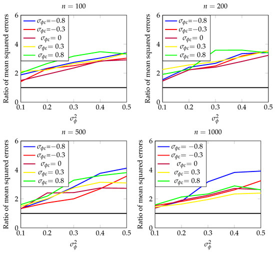
Figure 1.
Ratio of mean squared errors for and , with sample sizes , , , and (out of 100 replications).
The ratio of mean squared errors serves as a comparative measure, where values exceeding 1 (>1) indicate that the second estimator performs better than the first. This comparison enables an assessment of the relative performance between the two estimators.
When analyzing the results presented in Table 1 and visualized in Figure 1, it is evident that all ratios of mean squared errors surpassed the threshold of 1. This observation underscores the superior efficiency of the estimator over across various parameter combinations.
These findings reinforce the validity and robustness of the simulation study, providing empirical evidence in support of the enhanced performance of the estimator in comparison to .
5. Real-World Data Examples
In this section, we apply the conditional least squares and weighted least squares methods to analyze the RCGARMA model, as discussed in previous sections. To illustrate our theoretical results, we utilize two real datasets obtained from R packages. Our initial focus is on estimating the GARMA (1,0) model with a random coefficient, expressed in matrix form, as follows:
To assess the performance of our methods, we execute the model 100 times and compute the ratio of mean squared errors for each example, as described below.
Example 1
(“Yearly Sunspot” Data). In this example, we consider the "Yearly Sunspot" dataset, which is available in R using the command data (sunspot.year), containing observations of the yearly sunspot number time series observed from 1700 to 1988. This dataset is often used to demonstrate time-series analysis techniques (for more details, see [30]).
The ratio of mean squared errors is calculated based on the quality of a predictor, as follows:
where and are, respectively, the output variable , calculated by the estimators and .
Example 2
(“NileMin” Data). The “NileMin” dataset contains historical observations of yearly minimal water levels of the Nile River from 622 to 1281, measured at the Roda gauge near Cairo. These data are used to study the variability of river flow and its impact on water resource management (more descriptions and details can be found in [31]).
In the case of the “NileMin” dataset, the ratio of mean squared errors is computed based on the quality of a predictor, as follows:
The results clearly indicate that the forecasted values obtained from the conditional weighted least squares method closely align with the observed datasets, indicating that this method surpasses the conditional least squares method. This close correspondence between the predicted and actual values underscores the effectiveness of the conditional weighted least squares approach in capturing the underlying patterns and dynamics inherent in yearly sunspot data and yearly minimal water levels in the Nile River data. Importantly, our analysis reveals that the performance of the conditional weighted least squares method surpasses that of the conditional least squares method. This indicates that the former method offers superior predictive capabilities, resulting in more accurate and reliable forecasts of yearly sunspot activity and yearly minimal water levels. These findings hold significant implications for the field of environmental research, as they highlight the potential of the conditional weighted least squares method to enhance our comprehension and predictive abilities in this domain.
6. Concluding Remarks
This paper introduces alternative methods for estimating the random parameters of the GARMA model, namely the conditional least squares estimation method and the weighted conditional least squares method. Both of these estimators demonstrate improved performance. To compare their effectiveness, we conducted a simulation study and examined two real-world data examples. Based on the results, we concluded that the weighted least squares estimator outperforms the conditional least squares estimator.
Author Contributions
Conceptualization, O.E.; methodology, O.E.; validation, R.E.H. and S.H.; writing—original draft, O.E.; writing—review & editing, R.E.H. and S.H.; visualization, R.E.H. and S.H.; supervision, R.E.H. All authors have read and agreed to the published version of the manuscript.
Funding
This research was funded by Le Centre National Pour la Recherche Scientifique et Technique [Scholarship].
Data Availability Statement
The original data presented in the study are openly available in R (version R-4.4.0) at [30,31].
Conflicts of Interest
The authors declare no conflict of interest.
Appendix A
#
#----------------- installing and loading packages
#
if(!require("stats4")){install.packages("stats4")};library(stats4)
if(!require("mnormt")){install.packages("mnormt")};library(mnormt)
if(!require("methods")){install.packages("methods")};library(methods)
if(!require("sn")){install.packages("sn")};library(sn)
if(!require("smoothmest")){install.packages("smoothmest")};library(smoothmest)
#
#-------------------initialisation and creation of variables
X<-matrix(0, n_tot,1)
e<-matrix(0, n_tot,1)
phi_t<-matrix(0, n_tot,1)
one <- matrix(1,test,1)
#######################################
d<- -0.3
covp<-0.8
phi<-0.2
test=100
n_tot=1000
m=n_tot-1
eta<-1
RMSE =c(one)
for(N in 1:test){
#
#-------phi_t ------#
phi_t = c(rnorm(n_tot, mean = 0, sd =sqrt(0.1) ))
#
#---------- Epsilone -------#
e <- c(rnorm(n_tot, mean = 0, sd =1 ))
#
#---------Gegenbauer polynomial C-------#
poly.geg=function (u, d, ordre) {
C_0 = 1
C = rep(0,ordre)
C[1] = 2 * d * u
C[2] = 2 * u * ((d - 1)/2 + 1) * C[1] - (2 * (d - 1)/2 + 1) * C_0
for (j in 3:ordre)
C[j] = 2 * u * ((d - 1)/j + 1) * C[j -1] - (2 * (d - 1)/j + 1) * C[j - 2]
psi = c(C_0, C)
return(psi)
}
C<-poly.geg(u=1,d=0.3,ordre=10^5)
#
#-----------definition of X_t----#
Y<-matrix(0,m,1)
runif(m)
for (n in 2:m)
{
X[1]<-X[1]+((phi+phi_t[1])*C[n-1]-C[n])*Y[n]
}
X[1]<-X[1]+e[1]+((phi+phi_t[1])-C[1])*Y[1]
for(t in 2:n_tot)
{
X[t]<-0
for (n in 2:m)
{
if(t-n>0){
X[t]<-X[t]+((phi+phi_t[t])*C[n-1]-C[n])*X[t-n]
}
if(t-n<=0){
X[t]<-X[t]+((phi+phi_t[t])*C[n-1]-C[n])*Y[n-t+1]
}
}
X[t]<-X[t]+((phi+phi_t[t])-C[1])*X[t-1]+e[t]
}
#
#-------Definition of the vector of past observations X(t-1)------
X1<-function(t)
{
X1<- matrix(0, m,1)
for(n in 1:m)
{
if(t-n>0){
X1[n]<-X[t-n]
}
if(t-n<=0){
X1[n]<-Y[n-t+1]
}
}
return(X1)
}
#
#---------Variance--------#
Var<-matrix(0,m,m)
Var[1,1]<-var(phi_t)
for(j in 2:m)
{
Var[1,j]<-C[j-1]%*%var(phi_t)
}
for(j in 2:m)
{
Var[j,1]<-C[j-1]%*%var(phi_t)
}
for (i in 2:m)
{
for(j in 2:m)
{
Var[i,j]<- C[i-1]%*%C[j-1]%*%var(phi_t)
}
}
#
#----------covariance----------#
Cov=matrix(0,m,1)
for(i in 2:m)
{
Cov[i]<- C[i-1]%*%covp
}
Cov[1]<-covp
alphatb<-matrix(0,n_tot,1)
for(t in 1:n_tot)
{
R=X1(t)
alphatb[t]<-1+2*t(R)%*%Cov+t(R)%*%Var%*%R
}
#
#---------definition of WLS estimator-------#
A<-matrix(0,m,m)
for(t in 1:n_tot)
{
Xt1<-X1(t)
A<-A+(Xt1%*%t(Xt1))/alphatb[t]
}
solve(A)
B<-matrix(0,m,1)
for(t in 1:n_tot)
{
Xt1<-X1(t)
B<-B+(Xt1%*%X[t])/alphatb[t]
}
ThetaW<-solve(A)*B
ThetaW
#
#----------definition CLS estimator--------#
AA<-matrix(0,m,m)
for(t in 1:n_tot){
Xt1<-X1(t)
AA<-AA+(Xt1%*%t(Xt1))
}
solve(AA)
BB<-matrix(0,m,1)
for(t in 1:n_tot)
{
Xt1<-X1(t)
BB<-BB+(X[t]*Xt1)
}
ThetaC<-solve(AA)*BB
ThetaC
Theta<-matrix(0,m,1)
Theta[1]<-phi-C[1]
for(n in 2:m)
{
Theta[n]<-phi*C[n-1]-C[n]
}
#
#--------Mean squared error of CLS estimator-------#
T<-mean((t(ThetaC-Theta)%*%(ThetaC-Theta)))
#--------Mean squared error of CLS estimator-------#
G<-mean((t(ThetaW-Theta)%*%(ThetaW-Theta)))
#-------- Ratio of Mean squared errors---------#
RMSE[N]=T/G
}
U=mean(RMSE)
References
- Albarracin, Y.; Alencar, A.; Ho, L. Generalized autoregressive and moving average models: Multicollinearity, interpretation and a new modified model. J. Stat. Comput. Simul. 2019, 89, 1819–1840. [Google Scholar] [CrossRef]
- Hunt, R.; Peiris, S.; Weber, N. Estimation methods for stationary Gegenbauer processes. Stat. Pap. 2022, 63, 1707–1741. [Google Scholar] [CrossRef]
- Darmawan, G.; Rosadi, D.; Ruchjana, B.; Pontoh, R.; Asrirawan, A.; Setialaksana, W. Forecasting COVID-19 in INDONESIA with various time series models. Media Stat. 2022, 15, 83–93. [Google Scholar] [CrossRef]
- Tsay, R.S. Conditional Heteroscedastic Time Series Models. J. Am. Stat. Assoc. 1987, 82, 590–604. [Google Scholar] [CrossRef]
- Nicholls, D.F.; Quinn, B.G. Random Coefficient Autoregressive Models: An Introduction; Springer: New York, NY, USA, 1982. [Google Scholar]
- Appadoo, S.S.; Ghahramani, M.; Thavaneswaran, A. Moment properties of some time series models. Math. Sci. 2005, 30, 50–63. [Google Scholar]
- McDonough, T.; McMahon, C.; Kotz, D.M. Handbook on Social Structure of Accumulation Theory; Edward Elgar Publishing: Cheltenham, UK, 2021. [Google Scholar]
- Beaumont, P.; Smallwood, A. Inference for estimators of generalized long memory processes. Commun. Stat. Simul. Comput. 2021, 52, 6096–6115. [Google Scholar] [CrossRef]
- Hossain, S.; Pandher, S.; Volodin, A. Generalized autoregressive moving average models: An efficient estimation approach. J. Stat. Comput. Simul. 2023, 93, 556–580. [Google Scholar] [CrossRef]
- Woodward, W.A.; Cheng, Q.C.; Gray, H.L. A k-factor GARMA long-memory model. J. Time Ser. Anal. 1998, 19, 485–504. [Google Scholar] [CrossRef]
- Benjamin, M.A.; Rigby, R.A.; Stasinopoulos, D.M. Generalized autoregressive moving average models. J. Am. Stat. Assoc. 2003, 98, 214–223. [Google Scholar] [CrossRef]
- Euloge, F.; Kouamé, O.H. Minimum distance estimation of k-factors GARMA processes. Stat. Probab. Lett. 2008, 78, 3254–3261. [Google Scholar]
- Ou Larbi, Y.; El Halimi, R.; Akharif, A.; Mellouk, A. Optimal tests for random effects in linear mixed models. Hacet. J. Math. Stat. 2021, 50, 1185–1211. [Google Scholar] [CrossRef]
- El Halimi, R. Nonlinear Mixed-Effects Models and Bootstrap Resampling: Analysis of Non-Normal Repeated Measures in Biostatistical Practice; VDM Publishing: Riga, Latvia, 2009. [Google Scholar]
- Henry, L.; Gray, N.F.Z.; Wayne, A.W. On generalized fractional processes. J. Time Ser. Anal. 1989, 10, 233–257. [Google Scholar]
- Magnus, W.; Obcrhettinger, F.; Soni, R.P. Formulas and Theorems for the Special Functions of Mathematical Physics; Springer: Berlin/Heidelberg, Germany; New York, NY, USA, 1966; pp. 337–357. [Google Scholar]
- Rainville, E.D. Special Functions; Macmillan: New York, NY, USA, 1960. [Google Scholar]
- Akharif, A.; Hallin, M. Efficient detection of random coefficients in autoregressive models. Ann. Stat. 2003, 31, 675–704. [Google Scholar] [CrossRef]
- Vervaat, W. On a stochastic difference equation and a representation of non-negative infinitely divisible random variables. Adv. Appl. Probab. 1979, 11, 750–783. [Google Scholar] [CrossRef]
- Mundlak, Y. Models with Variable Coefficients: Integration and Extension. In Annales de l’INSEE; Institut National de la Statistique et des Études Économiques: Montrouge, France, 1978; pp. 483–509. [Google Scholar]
- Dissanayake, G.S.; Peiris, M.S.; Proietti, T. Fractionally Differenced Gegenbauer Processes with Long Memory: A Review. Statist. Sci. 2018, 33, 413–426. [Google Scholar] [CrossRef]
- Hwang, S.Y.; Basawa, I.V. Parameter estimation for generalized random coefficient autoregressive processes. J. Stat. Plan. Inference 1998, 68, 323–337. [Google Scholar] [CrossRef]
- Hwang, S.Y.; Basawa, I.V. Parameter estimation in a regression model with random coefficient autoregressive errors. J. Stat. Plan. Inference 1993, 36, 57–67. [Google Scholar] [CrossRef]
- Smith, J.; Johnson, R.; Brown, A. Robust Parameter Estimation in Generalized Autoregressive Moving Average Models with Random Effects. J. Stat. Model. 2020, 15, 101–115. [Google Scholar]
- Brown, C.; Lee, E. Addressing Unobserved Heterogeneity and Time-Varying Dynamics in Generalized Autoregressive Moving Average Models with Random Effects Using Least Squares Estimation. J. Appl. Econom. 2019, 24, 145–159. [Google Scholar]
- Jones, L.; Smith, K. Enhancing Interpretability in Generalized Autoregressive Moving Average Models with Random Effects Using Conditional Least Squares Estimation. J. Time Ser. Anal. 2018, 12, 201–215. [Google Scholar]
- Billingsley, P. The Lindeberg-Lévy Theorem for Martingales. Proc. Am. Math. Soc. 1961, 12, 788–792. [Google Scholar]
- Ngatchou-Wandji, J. Estimation in a class of nonlinear heteroscedastic time series models. Electron. J. Stat. 2008, 2, 46–62. [Google Scholar] [CrossRef]
- Slutsky, E. Über stochastische Asymptoten und Grenzwerte. Tohoku Math. J. First Ser. Metron 1926, 27, 67–70. (In German) [Google Scholar]
- Tong, H. Non Linear Time Series; Clarendon Press: Oxford, UK, 1996; p. 471. [Google Scholar]
- Tousson, O. Mémoire sur l’Histoire du Nil; Mémoire de l’Institut d’Egypte: Cairo, Egypt, 1925. [Google Scholar]
Disclaimer/Publisher’s Note: The statements, opinions and data contained in all publications are solely those of the individual author(s) and contributor(s) and not of MDPI and/or the editor(s). MDPI and/or the editor(s) disclaim responsibility for any injury to people or property resulting from any ideas, methods, instructions or products referred to in the content. |
© 2024 by the authors. Licensee MDPI, Basel, Switzerland. This article is an open access article distributed under the terms and conditions of the Creative Commons Attribution (CC BY) license (https://creativecommons.org/licenses/by/4.0/).