Optimizing Variational Quantum Neural Networks Based on Collective Intelligence

Abstract

Quantum machine learning stands out as one of the most promising applications of quantum computing, widely believed to possess potential quantum advantages. In the era of noisy intermediate-scale quantum, the scale and quality of quantum computers are limited, and quantum algorithms based on fault-tolerant quantum computing paradigms cannot be experimentally verified in the short term. The variational quantum algorithm design paradigm can better adapt to the practical characteristics of noisy quantum hardware and is currently one of the most promising solutions. However, variational quantum algorithms, due to their highly entangled nature, encounter the phenomenon known as the “barren plateau” during the optimization and training processes, making effective optimization challenging. This paper addresses this challenging issue by researching a variational quantum neural network optimization method based on collective intelligence algorithms. The aim is to overcome optimization difficulties encountered by traditional methods such as gradient descent. We study two typical applications of using quantum neural networks: random 2D Hamiltonian ground state solving and quantum phase recognition. We find that the collective intelligence algorithm shows a better optimization compared to gradient descent. The solution accuracy of ground energy and phase classification is enhanced, and the optimization iterations are also reduced. We highlight that the collective intelligence algorithm has great potential in tackling the optimization of variational quantum algorithms.

1. Introduction

With the rapid development of quantum technology, algorithms applied to noisy medium-scale quantum systems are becoming more and more efficient. Variational quantum algorithms mainly rely on the optimization of parameter quantum circuits and are the most promising application-oriented technologies. Two early applications of variational quantum algorithms are variational quantum solvers and quantum approximate optimization algorithms. In addition to applications in quantum chemistry and combinatorial optimization, variational quantum algorithms have recently been applied to various machine learning problems, such as pattern recognition, information compression, and the generation of artificial intelligence models [1,2,3,4].

Variational quantum neural networks (QNNs) can run on various quantum hardware configurations and can handle the ground state resolution and combinatorial optimization problems in graph theory. Variational quantum algorithms mainly consist of four parts: variational quantum state preparation, quantum state operation, measurement, and parameter optimization. The parameter optimization part uses classical optimizers for optimization, while the variational quantum circuit is mainly used to create the quantum state wave function to be optimized. By repeatedly measuring the quantum state, the optimization process estimates the expectation value of a specific Hermitian operator relative to the current wave function to be optimized. When the object function is finally minimized, it is time to perform parameter optimization and training.

Recent studies have shown that, as the number of quantum bits increases, the gradient gradually decreases to zero, thereby affecting the optimization of parameterized quantum circuits, which is the so-called “barren plateau” problem [5,6,7,8,9]. This problem means that random initialization will cause gradient-based optimization techniques to fail in a large class of circuits. The scalability of variational quantum feature solvers and QNN and other variational quantum algorithms depends on whether a solution to the problem can be found. Many recent studies have tried to solve the barren plateau problem. Stokes et al. proposed quantum natural gradients for parameterized quantum circuits [10], which are expected to provide advantages over existing stochastic optimization methods. By reducing the unpredictability and depth of the circuit, the literature [11] created an initialization technique for solving the barren plateau problem in deep circuits. The literature [12] proposed defining a weak barren plateau based on the local approximate value of the density matrix entropy and believed that, to avoid a weak barren plateau, a larger initialization gradient should be ensured. The academic community generally believes that the barren plateau will directly affect gradient-based optimizers [6,9]. Optimizers that rely on higher-order derivatives will also be affected, as their size will exponentially decay in the barren plateau loss landscape.

Therefore, this paper proposes using gradient-free optimization to train parameterized quantum circuits. Population intelligence optimization methods are not limited to using local gradient information, but can use global information about the loss landscape. They represent a class of different high-dimensional problem solutions called feasible black-box optimization methods, which are very suitable for nonlinear, non-convex, or non-smooth optimization problems. Chen et al. [13] proposed two deep quantum reinforcement learning task frameworks using gradient-free evolution optimization, providing insights into recent quantum reinforcement learning. Anand et al. [14] proved that using intelligent optimization can mitigate the exponential decay of variance during quantum circuit training. In [15], the authors demonstrated the application of stochastic gradient descent and heuristic algorithms in the optimization of deep neural networks, and proved that they can achieve state-of-the-art performance based on the complementarity between gradient descent and intelligent algorithms.

This paper proposes a quantum neural network optimization method based on the particle swarm optimization algorithm. The particle swarm optimization algorithm is a heuristic optimization method based on the observation of collective behavior in nature, which simulates the cooperative behavior of individuals in the search space to find the optimal solution. Its inspiration comes from observing the collective movements of organisms such as flocks of birds and schools of fish, where individuals enhance overall performance through mutual communication and cooperation. The variational quantum neural network algorithm based on particle swarm optimization can mitigate the barren plateau problem in variational quantum circuits, thereby accelerating the training efficiency and convergence speed of the network.

2. Physical Model and Methods

2.1. Variational Quantum Neural Networks

Qubits form the foundation of variational QNNs, where a single qubit superposition can be represented as $|\varphi \rangle =\alpha |0\rangle +\beta |1\rangle$, where $\alpha$ and $\beta$ are complex numbers. Quantum gates are the basic units that operate on qubits. Common quantum gates include the $X,Y,Z$, and CNOT gates. In the NISQ era, commonly used quantum operations, in addition to the four quantum logic gates, also include rotation gates such as single-qubit rotation gates $R_X,R_Y,R_Z$, and two-qubit parameterized gates $R_{XX},R_{YY},R_{ZZ}$.

QNNs are primarily composed of parameterized Pauli rotation gates. In consideration of practical hardware characteristics, two-qubit gates can only be applied directly on adjacent qubits. For two-qubit operations between non-adjacent qubits, swap operators are employed to exchange the positions of qubits. However, such operations inevitably increase the overhead of quantum circuits. Common variational quantum neural networks are constructed by interleaving single-qubit rotation layers with two-qubit entanglement layers. This quantum circuit topology fully considers practical hardware characteristics and is also referred to as hardware-efficient quantum circuit topology. In general, a randomly parameterized quantum circuit can be mathematically represented as

$$U\left(\theta \right)=U({\theta }_1,{\theta }_2,\cdots ,{\theta }_L)=\prod _{l=1}^L{U}_l\left({\theta }_l\right)W_l,$$

(1)

where $U_l\left({\theta }_l\right)=exp(-i{\theta }_l{H}_l)$, ${\theta }_l$ is a real training parameter, $H_l$ denotes an arbitrary Hermitian operator, an $W_l$ is the untrainable unitary operator. Suppose there is an observable M and the initial quantum state is the zero state: the expectation value of the final quantum state after the operation of the QNN is given by

$$E\left(\theta \right)=\langle 0\left|U^{†}\left(\theta \right)MU\left(\theta \right)\right|0\rangle .$$

(2)

The schematic diagram of the variational quantum neural network is shown in Figure 1. From the diagram, it turns out that the quantum neural network is essentially a complex unitary transformation. By transforming the zero state into a parameterized quantum state and then measuring it, we can obtain features about the parameters and calculate the loss function. In general, the expectation value of the observable $M={[\langle Z_1\rangle ,\langle Z_2\rangle ,\cdots ,\langle Z_n\rangle ]}^T$ represents an n-dimensional classical feature vector derived from the variational QNN. For combinatorial optimization problems, the optimal solution of the optimization problem can be extracted from this feature vector.

In machine learning applications, classical features can usually be converted into a quantum superposition form through different encoding methods such as angle encoding [16] and amplitude encoding [17,18], and then processed using the parameterized QNN. The process of classical feature encoding into quantum states can also be represented as a unitary transformation, denoted by $W_l$. To further enhance the learning and training capabilities of QNNs after obtaining quantum features, classical neural networks can be used for re-learning on quantum features. This hybrid architecture can effectively improve the optimization ability of QNNs.

2.2. Barren Plateau Problem

When the training parameters are randomly initialized, the gradients of parameterized loss function $E\left(\theta \right)$ over $\theta$ can be written as

$${\mathsf{\partial }}_{k}E=\frac{\mathsf{\partial }E\left(\theta \right)}{\mathsf{\partial }{\theta }_k}=i\langle 0|U_{-}^{†}[H_k,U_{+}^{†}H{U}_{+}]U_{-}|0\rangle ,$$

(3)

where $U_{-}={\prod }_{l=k-1}^1{U}_l\left({\theta }_l\right)W_l,U_{+}={\prod }_{l=L}^k{U}_l\left({\theta }_l\right)W_l$. In theory, when $U_{-}$ and $U_{+}$ satisfy a second-order Haar random distribution, i.e., a two-design [5], the Hilbert dimension can exponentially suppress the magnitude of the gradients. In other words, we need an exponentially scaled number of samples or measurements to estimate the gradients. This effect can hinder the practical utility of QNNs in wide applications.

To evaluate the expected value of the gradient of the loss function to the parameter under the Haar random unitary matrix of a particular distribution, it can be defined as

$$\langle {\mathsf{\partial }}_{k}E\rangle =\int \mathrm{d}Up\left(U\right){\mathsf{\partial }}_k\langle 0|U^{†}\left(\theta \right)HU\left(\theta \right)|0\rangle ,$$

(4)

where $p\left(U\right)$ denotes the likelihood distribution of the unitary operator U. In theory, when the distributions are truly Haar random, the gradients of the loss function over $\theta$ should be zero. As the QNNs are deep enough and $U_{-},U_{+}$ and ${\mathsf{\partial }}_{k}E$ are two-design, the phenomenon of the barren plateau is certain to occur. In other words, the variance of the parameter gradient appears to decay exponentially as the system scale rises, at which point, it is not possible to find a suitable direction of the gradient descent for optimization in the optimization landscape. Therefore, we make use of shallow quantum circuits as the QNN, rather than a deep one if the expressive power is enough to solve our problem.

2.3. Quantum Optimization Algorithms Simulated by Classical Computers

Conventional QNN optimization simulated by classical computers can be categorized into two types: automatic differentiation and parameter shift differentiation. For automatic differentiation, this approach can only be applied to tensor simulation software for quantum circuits, such as TorchQuantum-0.1.8, Tensorflow Quantum [19], and so on. However, it is worth noting that the number of qubits supported by quantum simulation software is relatively limited because the computational overhead also grows exponentially with the number of qubits. In the classical machine learning field, automatic differentiation is also known as gradient backpropagation, and this technology lays the foundation for the efficient training of large-scale deep learning models [20].

2.4. Particle Swarm-Based Quantum Optimization Algorithm

For real quantum hardware, since there are currently no quantum algorithms that support automatic differentiation, the parameter shift rule is used to calculate parameter gradients. This method is essentially a differential method for gradient calculation. For the QNN transformation, assuming the parameter set $\theta =[{\theta }_1,\cdots ,{\theta }_i,\cdots ,{\theta }_n]$ denotes the training quantum parameters of a QNN, the quantum circuit can be given by

$$f\left(\theta \right)=\langle \varphi |U^{†}\left({\theta }_i\right)QU\left({\theta }_i\right)|\varphi \rangle ,f\left(\theta \right)\in {\mathbb{R}}^m,\theta \in {\mathbb{R}}^n,$$

(5)

where $U\left({\theta }_i\right)$ denotes the quantum operation of the i-th parameter. For clarity, we absorb the operators before $U\left({\theta }_i\right)$ into $\left(\varphi \right|\varphi )$, and denote the operation of $U\left({\theta }_i\right)$ and the observable as operator Q. In order to calculate the gradient of ${\theta }_i$, we can make us of the parameter shift rule [21] to obtain the approximate gradients. It turns out that Pauli operator-generated quantum gates only have two eigenvalues with $+1$ and $-1$; therefore, according to the parameter shift rule, we have

$$\frac{\mathsf{\partial }f\left(\theta \right)}{\mathsf{\partial }{\theta }_i}=\frac{1}{2}[f\left({\theta }_{+}\right)-f\left({\theta }_{-}\right)],$$

(6)

where ${\theta }_{+}=[{\theta }_1,\cdots ,{\theta }_i+\pi /2,\cdots ,{\theta }_n],{\theta }_{-}=[{\theta }_1,\cdots ,{\theta }_i-\pi /2,\cdots ,{\theta }_n]$ denotes the positive shift and negative shift of the parameter vectors, respectively.

Gradient-based optimization algorithms can optimize shallow variational quantum neural networks. However, for deep QNNs, there exists the problem of barren plateaus, which results in reduced optimization efficiency. Optimization methods based on the particle swarm algorithm utilize the concept of swarm intelligence [22]. They do not require gradient calculations to optimize the target loss function, although this depends on the evaluation of the target function by individuals in the swarm. Each parameter in the QNN can be regarded as an individual in the swarm, with each individual having two intrinsic attributes: position X and velocity S:

Step1.

Algorithm initialization. Initially, each parameter is initialized with an initial position and initial velocity, that is each set of parameters ${\theta }_i$ is updated to $(X_i,S_i)$. Apart from the initial condition, individual historical best positions $P_{\mathrm{best}}$ and group best position $G_{best}$ are also recorded for each parameter. The individual best position is used to optimize individual parameters, while the group best position is responsible for optimizing the global parameter vector. Generally, the more particles initialized, the higher the search efficiency and the better the optimization results. However, when setting a larger number of particles, there will be a problem of high computational cost in evaluating the fitness of each particle. Therefore, a good balance between the number of particles and optimization overhead needs to be considered.

Step2.

Optimize swarms. For each parameter vector ${\theta }^i$, its update rule is as followed:

(a)

Speed update:

$$S_i(t+1)=w{S}_i\left(t\right)+c_1{r}_1(P_{\mathrm{best}}^i-X_i\left(t\right))+c_2{r}_2(G_{\mathrm{best}}-X_i\left(t\right)).$$

(7)

(b)

Position update:

$$X_i(t+1)=X_i\left(t\right)+S_i(t+1).$$

(8)

where w is the inertia weight, usually set between $[0.4,0.9]$. The larger the inertia weight, the higher the global optimization capability is. In our implementation, we make use of an adaptive weight varying with the number of iterations. For example, suppose the total number of iterations is T, the current iteration is t, then the weight can be updated by

$$w_t=0.9-(0.9-0.4)\times \frac{t}{T}.$$

$c_1$ and $c_2$ are the weights of the acceleration terms, usually taken as positive values, and $r_1$ and $r_2$ are random numbers between $[0,1]$.

Step3.

Fitness evaluation. Compute the fitness of each parameter vector, and compare it with the individual historical best position $P_{\mathrm{best}}^i$. In case the current position’s fitness is better than the individual historical best position, then update $P_{\mathrm{best}}^i$; otherwise, do not update. The specific fitness function can be characterized using the quantum loss function $E\left(\theta \right)$.

Step4.

Global update. Compare the individual historical best positions of all particles with the overall group historical best position. If the individual historical best position of a particle is better than the overall group historical best position, then update the overall group historical best position to the position of that particle.

Step5.

Convergence condition. Repeat steps 1–4 until the termination condition is met, such as reaching the maximum number of iterations or satisfying a specific fitness threshold.

In our proposed quantum optimization, particle positions can be regarded as the numerical values of parameter vectors. The position update is essentially the parameter update. For machine learning tasks, since there is a batch optimization step, different batches of samples need to be optimized within one round. Therefore, for each batch, a termination iteration number needs to be determined.

3. Results

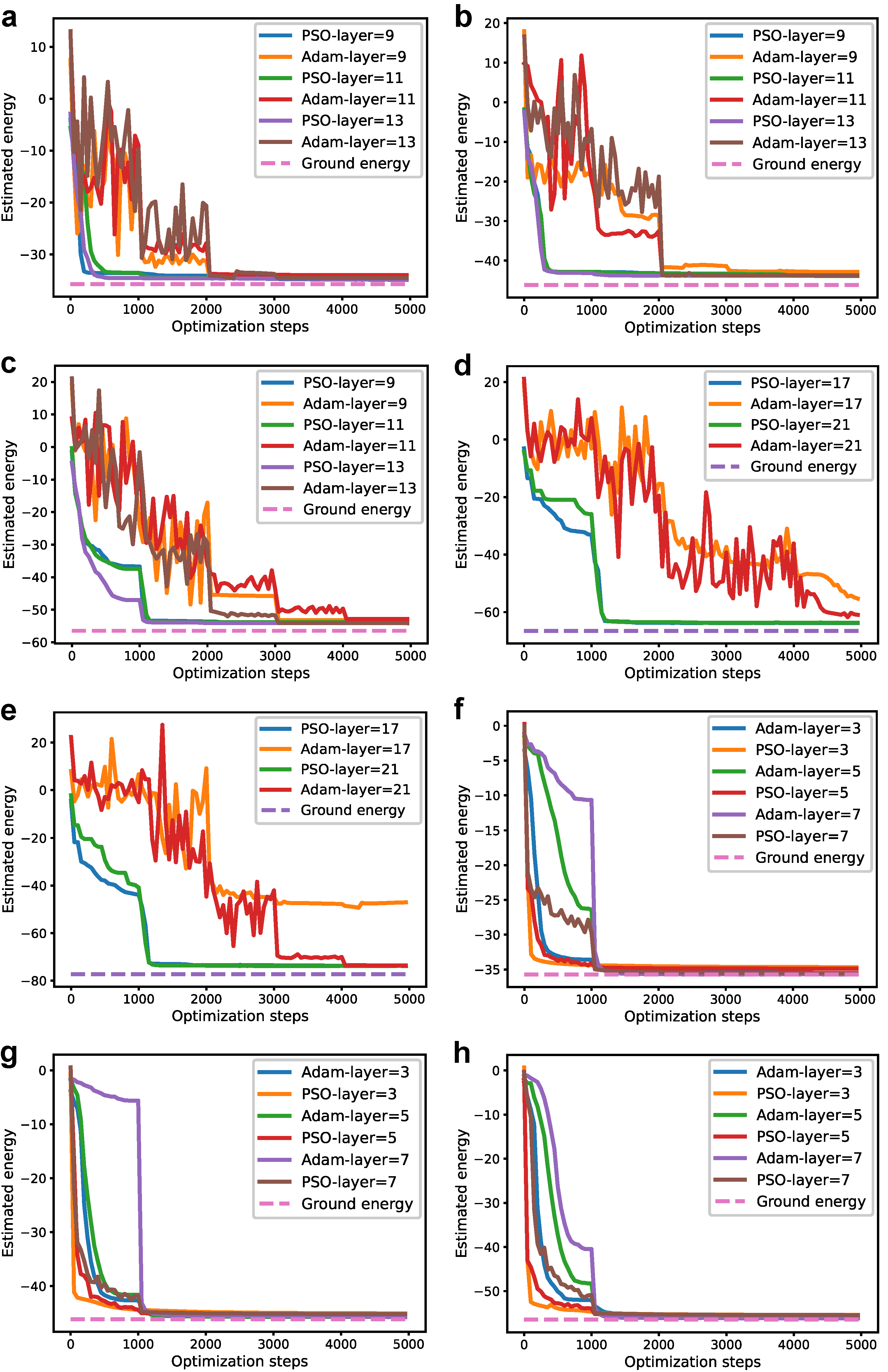
3.1. Solving Ground Energy of a Two-Dimensional Random Hamiltonian

The ground state of a Hamiltonian is one of the most important applications of variational quantum algorithms in the field of quantum chemistry. Consider the Heisenberg-XYZ model; its mathematical expression is given by

$$H=\sum _i{Z}_i+\sum _{\langle i,j\rangle }{\alpha }_{ij}{Z}_i\otimes Z_j+\sum _{\langle i,j\rangle }{\alpha }_{ij}(X_i\otimes X_j+0.66Y_i\otimes Y_j),$$

(9)

where $\langle i,j\rangle$ denotes the index of neighboring qubits and ${\alpha }_{ij},{\beta }_{ij}$ are randomly sampled values from a Gaussian distribution. The mean value is set to be 1 and 3, respectively, and the variance is set to be $0.25$. In theory, the ground energy of the random Hamiltonian H can be calculated through variationally minimizing the following equation, that is

$${\theta }^{★}=argminE\left(\theta \right)=\langle \varphi \left(\theta \right)\left|H\right|\varphi \left(\theta \right)\rangle ,$$

(10)

where we have $\left|\varphi \right(\theta )\rangle =U(\theta \left)\right|0\rangle$. The quantum circuit structure of the QNN makes use of a hardware-efficient topology. More formally, the l-th layer of the hardware-efficient QNN is given by

$$U_l\left({\theta }_l\right)=\underset{i}{⨂}{R}_{ZZ}^i\left({\theta }_{le}\right)\underset{i}{⨂}{R}_Z^i\left({\theta }_{l1}\right)R_Y^i\left({\theta }_{l2}\right)R_Z^i\left({\theta }_{l3}\right),$$

(11)

where $R_{ZZ}$ is the two-qubit entanglement gate, and it acts on any two neighboring qubits. Note that the lth layer parameter is denoted as ${\theta }_l=({\theta }_{le},{\theta }_{l1},{\theta }_{l2},{\theta }_{l3})$, where ${\theta }_{le}$ is the entanglement parameter and ${\theta }_{l1},{\theta }_{l2},{\theta }_{l3}$ are single-qubit gate quantum parameters. It is worth noting that the arbitrary single-qubit gate can be decomposed into the composition operation $R_Z^i\left({\theta }_{l1}\right)R_Y^i\left({\theta }_{l2}\right)R_Z^i\left({\theta }_{l3}\right)$. Note that, in Figure 1, we do not use the $R_{ZZ}$ gate to express the entanglement operation. However, $R_{ZZ}$ can be decomposed into two CNOT gates and a single $R_Z$ gate. Using multi-layer variational quantum circuits, the expressive power of variational quantum neural networks can be greatly enhanced. For the Heisenberg-XYZ model, the hardware-efficient topology shown above is more efficient [23,24,25,26,27], as shown in Figure 2a.

Another option is to use the chessboard quantum circuit structure assumption to construct the ground state wavefunction, as shown in Figure 2b. In theory, each two-qubit gate contains 15 parameters, enabling the construction of arbitrary two-qubit gates.

To compare and analyze the abilities of the gradient descent algorithm and PSO algorithm in solving the ground state of quantum Hamiltonians, simulations were conducted for different quantum circuits with varying qubit counts and depths, as shown in Figure 3. When using hardware-efficient quantum circuits, the numerical results in Figure 3a–c indicate that the PSO algorithm exhibits faster convergence compared to the gradient descent algorithm. Furthermore, as the depth increases, both the PSO and gradient descent algorithms show reduced convergence. In Figure 3d,e, we further increase the number of qubits and layers used to demonstrate the advantage of PSO over gradient descent methods in terms of convergence speed. The results show that PSO has achieved clear advantage over the Adam method, in the early stage of the optimization. During the late state, both methods converge to the ground energy. In Figure 3f–h, we make use of the checkerboard ansatz to run the quantum circuit. We notice that PSO still has better convergence speed especially in the early state of the training, although both methods achieve good convergence. In addition, checkerboard ansatz is in principle harder to optimize than the hardware-efficient ansatz since each unitary block of the two-qubit gate is an SU(4) with 15 free parameters. When the initial parameter is not properly initialized, they are hard to optimize [28].

However, PSO still demonstrates clear advantages over gradient descent. Under these conditions, the number of parameters in the variational quantum neural network remains moderate. However, neither algorithm converges to the optimal ground state energy when using hardware-efficient quantum circuit configurations. Therefore, to investigate the ground state-solving capability of variational quantum neural networks, chessboard quantum circuit configurations were employed. The parameter space of chessboard quantum circuit configurations is larger compared to hardware-efficient quantum circuit configurations, leading to higher-dimensional parameter spaces.

The numerical analysis using the PSO and gradient descent algorithms revealed that PSO maintains a faster convergence rate compared to gradient descent, even with increased circuit depth and qubit count. However, both algorithms exhibit decreased convergence rates as the depth and qubit count increase. From the simulation results, it is evident that PSO is less affected by these factors, showcasing its potential in non-convex high-dimensional optimization and its adaptability in optimizing the parameters of variational quantum neural networks. Since PSO does not rely on gradient computation, it can quickly find suitable parameters, thereby approximating the ground state energy closer to the true value. Therefore, in future real quantum circuits, the PSO algorithm can be a promising candidate.

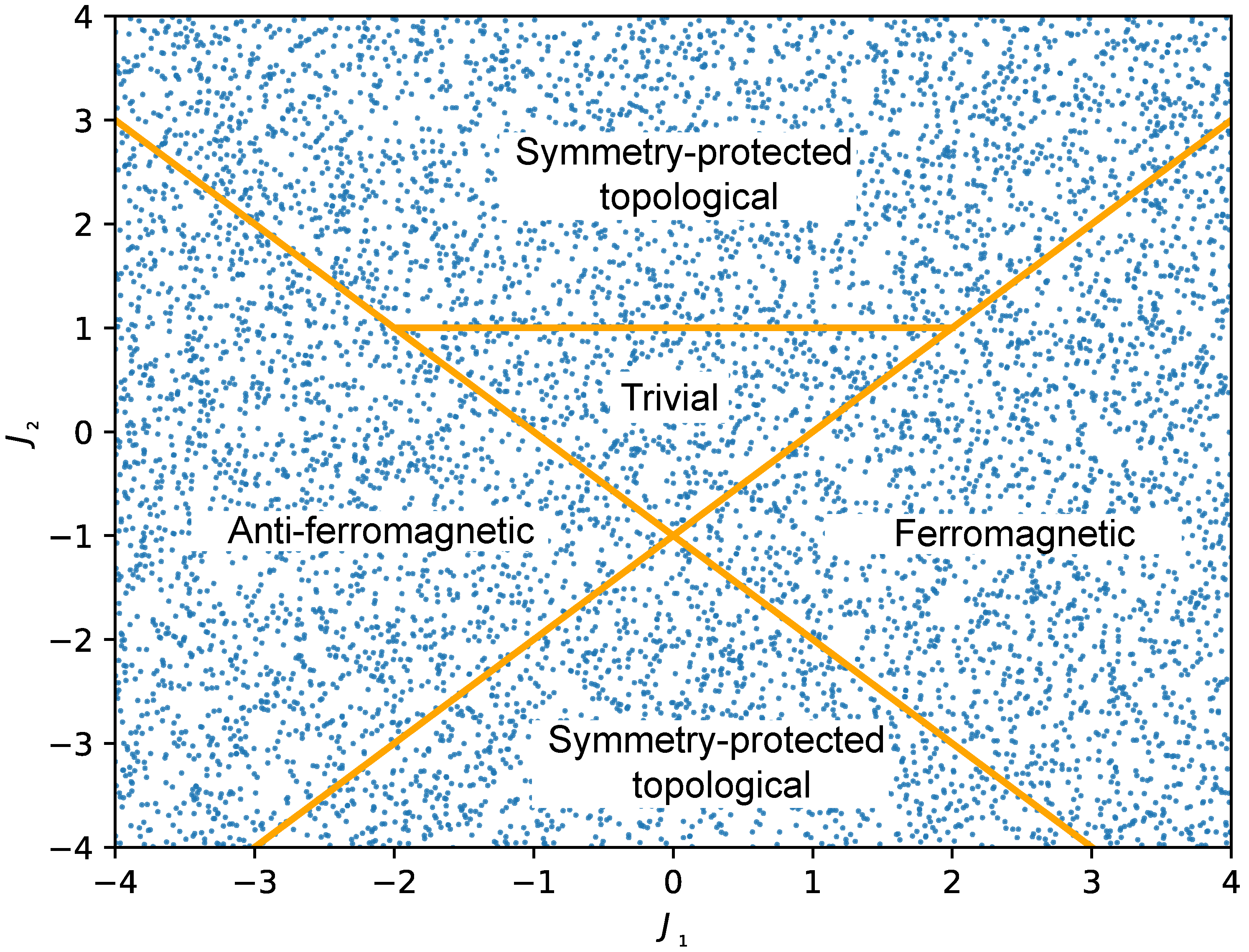
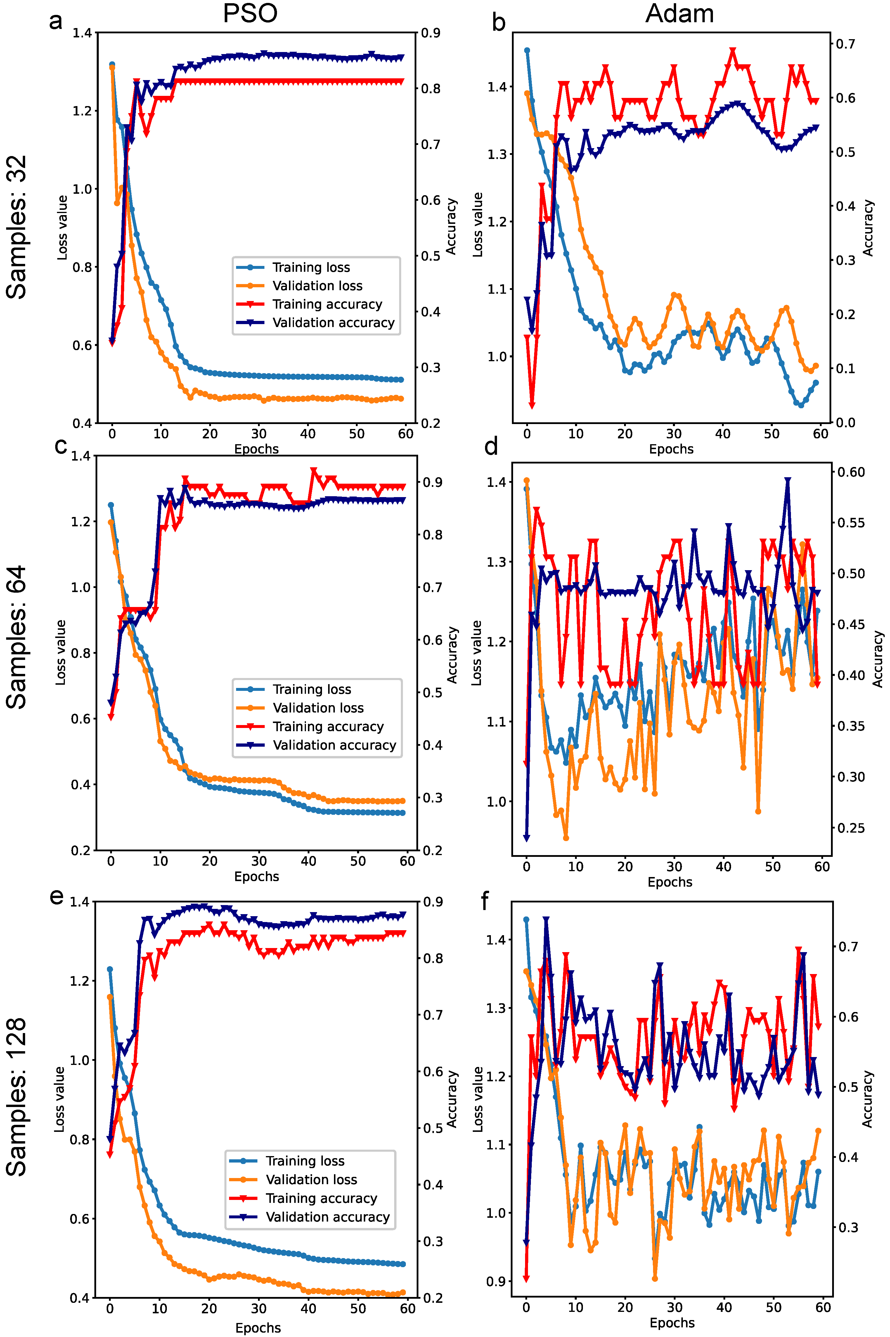
3.2. Quantum Phase Classification

In this case, we make use of quantum convolutional neural networks to classify quantum phases of a many-body system. A general QCNN structure is shown in Figure 4. The QCNN consists of three typical structures: convolution, pooling, and fully connected layer [29]. These three structures are similar to classical convolution neural network. The input of the QCNN is the ground state (pure state or density matrix) of a Hamiltonian model, and the output is its phase label. Through the end-to-end supervised training, the trained QCNN can automatically recognize the phase label of an unknown ground state of the same Hamiltonian. Also, the action of a QCNN can be viewed as a mapping that maps the input state ${\rho }_{\mathrm{in}}$ to an output state ${\rho }_{\mathrm{out}}$ with ${\rho }_{\mathrm{out}}={\mathcal{E}}_{\theta }^{\mathrm{QCNN}}\left({\rho }_{\mathrm{in}}\right)$, where $\theta$ is the variational parameters. Then, given ${\rho }_{\mathrm{out}}$, one measures the expectation value of a specific Hermitian operator to obtain the final phase label.

In our implementation, we consider the cluster Hamiltonian given by

$$H_{XXZ}=\sum _{j=1}^n(Z_j-J_1{X}_j{X}_{j+1}-J_2{X}_{j-1}{Z}_j{X}_{j+1}),$$

(12)

where n denotes the number of qubits, $Z_j$$\left(X_j\right)$ denotes the Pauli $z\left(x\right)$ operator acting on qubit j, and $J_1,J_2$ are tunable coupling parameters. As analyzed in [30], the phase diagram is shown in Figure 5. There are four phases: (1) symmetry-protected topological, (2) ferromagnetic, (3) anti-ferromagnetic, and (4) trivial. The classical simulation can be conducted by exact diagonalization for small systems, e.g., the number of qubits is smaller than 20.

To construct the training set, we sample from the two-dimensional parameter space $(J_1,J_2)$. For each parameter vector, its corresponding ground state is calculated and its phase label is assigned. The training set is composed of $\{\left(\right|{\varphi }_i\rangle ,y_i){\}}_{i=1}^N$, where the ground state is denoted as $|{\varphi }_i\rangle$ and the phase label is $y_i\in {\{0,1\}}^2$ with each bitstring corresponding to a phase that $|{\varphi }_i\rangle$ belongs to. We define the loss function as

$$\mathcal{L}(\theta ;|{\varphi }_i\rangle ,y_i)=\langle y_i|{\mathcal{E}}_{\theta }^{\mathrm{QCNN}}\left(\right|{\varphi }_i\rangle \langle {\varphi }_i\left|\right)|y_i\rangle .$$

(13)

In the training process, we are required to minimize the loss function to obtain the optimal variational parameters $\theta$. We define the classification accuracy, which is give by

$$\mathrm{Accuracy}=\frac{{\sum }_{\left(\right|{\varphi }_i\rangle ,y_i)\in D}{\widehat{I}}_{y_i={\widehat{y}}_i}}{|D},D=D_{\mathrm{T}}\mathrm{or}{D}_{\mathrm{V}},$$

(14)

where ${\widehat{I}}_{y_i={\widehat{y}}_i}$ denotes the indicator variable, which equals 1 if $y_i={\widehat{y}}_i$, otherwise 0, $\left|D\right|$ denotes the number of samples in the dataset, and $D_{\mathrm{T}}$ and $D_{\mathrm{V}}$ are the datasets for training and validation.

We evaluate the performance when classifying the phases under different training samples and number of qubits. The numerical results are shown in Figure 6. In Figure 6a,b, the number of training samples is 32, in (c,d) is 64, and in (d–f) is 128. We note that the number of qubits in the QCNN is 12. We can find that, when the number of qubits is fixed, more training samples are not necessary to increase the accuracy. Small training sampling can also perform well in quantum phase classification. It also demonstrates that the QCNN has a strong ability in classifying quantum phases even with a highly small number of training sample. More importantly, Figure 6a,c,e are optimized based on the PSO algorithm with a full batch size. Figure 6b,d,f are optimized based on Adam with a learning rate of 0.001 and a batch size of four. When the number of training sampling is small, i.e., 32, the Adam algorithm can also converge normally. However, when the training sampling becomes large, the optimization of the QCNN becomes harder. The conventional Adam method cannot converge normally. In contrast, the PSO algorithm can still optimize the QCNN parameters normally. Besides, the accuracy of the QCNN optimized by the PSO is also higher than the Adam-optimized QCNN. Therefore, we can conclude that collective intelligence algorithms such as PSO have a stronger optimization ability when dealing with QCNN training. We also conducted numerical results when the number of qubits is varied. The results are presented in

Table 1. The final validation accuracy of PSO and Adam in optimizing the QCNN with 300 epochs under different numbers of qubits $\left(n\right)$ and training samples $\left(N\right)$.

	$\mathit{N}=32$	$\mathit{N}=64$	$\mathit{N}=128$
$n=12$ (PSO)	0.82	0.89	0.84
$n=12$ (Adam)	0.50	0.51	0.53
$n=14$ (PSO)	0.86	0.87	0.873
$n=14$ (Adam)	0.51	0.512	0.55
$n=16$ (PSO)	0.90	0.92	0.95
$n=16$ (Adam)	0.53	0.537	0.544

.

From Table 1, we can find that, when the number of qubits is large in the QCNN, the accuracy is higher when using the PSO algorithm. It can be clarified that, when quantum space is larger, more quantum parameters are used to classify the quantum phases. Therefore, the accuracy is higher than the small number of qubits. However, the Adam algorithm still has difficulty optimizing the QCNN in a good manner. The classification accuracy is lower than the PSO-optimized QCNN. The results also demonstrate that quantum neural networks are hard to optimize. Using PSO algorithms, the optimization ability can be greatly enhanced.

4. Simulation Environment and Hyperparameters

We used TensorCircuit [31] and PyTorch [32] as our simulation environments for both optimization methods studied. The hyperparameters of PSO are listed below.

The initial weight was set to $0.9$. The number of the particles was set to 64. The cognitive coefficient, which is $c_1$ in Equation (7), is $0.5$. The social coefficient, which is $c_2$ in Equation (7), was set to $0.5$. The max value of the parameters in the search space was set to $0.5$, and the min value was set to $-0.5$.

One main hyperparameter of Adam is the learning rate, and other hyperparameters remained unchanged in the PyTorch software. Here, we set the learning rate to 0.001. It turns out that, in practical implementation, we do not require paying much attention to optimizing the hyperparameters. As PSO has a stronger global optimization ability, it is highly suitable to optimize the variational quantum circuits with SU(4) blocks. Therefore, the results are reasonable and are not caused by the hyperparameters.

5. Conclusions

This paper investigates the potential of variational quantum neural networks based on swarm intelligence algorithms, namely PSO, in solving the ground state of complex two-dimensional Hamiltonians and in classifying quantum phases using the QCNN. In addressing the problem of finding the ground state of two-dimensional random Hamiltonians, it is observed through numerical analysis and comparison of the results obtained under different quantum circuit configurations that various numbers of qubits and diverse circuit depths that the PSO algorithm demonstrates superior convergence efficiency and optimization capability. Additionally, due to its independence from parameter gradients and potential robustness to noise in quantum circuits, the PSO algorithm can be employed for optimizing future quantum circuits and for solving and analyzing ground-state Hamiltonians, thereby expediting the discovery of new materials and similar applications.

In the research on classifying quantum phases using QCNNs, by analyzing the classification accuracy of the PSO algorithm and the Adam algorithm under various conditions of quantum bits and training sample sizes, it is found that the PSO algorithm enhances the training efficiency and improves the classification accuracy of QCNNs. In contrast, the Adam algorithm fails to sufficiently optimize the QCNN parameters, resulting in lower classification accuracy compared to the PSO algorithm. For future research directions, it is recommended to fully exploit the advantages of combining swarm intelligence algorithms with gradient descent algorithms to propose and develop hybrid optimization schemes. This would further enhance the optimization capability of quantum circuits and establish a solid foundation for the application of variational quantum circuits [33,34]. PSO can aid in optimizing the parameters of quantum circuits or variational quantum algorithms to accurately simulate quantum systems. This can have implications for various fields, including quantum chemistry and materials science, and has potential to be applied in quantum machine learning, quantum optimization algorithms, and quantum simulation when real quantum computers are invented.

References

1. Preskill, J. Quantum computing in the NISQ era and beyond. arXiv 2018, arXiv:1801.00862v3. [Google Scholar] [CrossRef]
2. McClean, J.; Romero, J.; Babbush, R.; Aspuru-Guzik, A. The theory of variational hybrid quantum-classical algorithms. New J. Phys. 2016, 18, 023023. [Google Scholar] [CrossRef]
3. Farhi, E.; Goldstone, J.; Gutmann, S. A quantum approximate optimization algorithm. arXiv 2014, arXiv:1411.4028. [Google Scholar] [CrossRef]
4. Cao, Y.; Guerreschi, G.G.; Aspuru-Guzik, A. Quantum neuron: An elementary building block for machine learning on quantum computers. arXiv 2017, arXiv:1711.11240. [Google Scholar] [CrossRef]
5. McClean, J.R.; Boixo, S.; Smelyanskiy, V.N.; Babbush, R.; Neven, H. Barren plateaus in quantum neural network training landscapes. Nat. Commun. 2018, 9, 4812. [Google Scholar] [CrossRef] [PubMed]
6. Arrasmith, A.; Cerezo, M.; Czarnik, P.; Cincio, L.; Coles, P.J. Effect of barren plateaus on gradient-free optimization. Quantum 2021, 5, 558. [Google Scholar] [CrossRef]
7. Cheng, B.; Deng, X.-H.; Gu, X.; He, Y.; Hu, G.; Huang, P.; Li, J.; Lin, B.-C.; Lu, D.; Lu, Y. Noisy intermediate-scale quantum computers. Front. Phys. 2023, 18, 21308. [Google Scholar]
8. Colless, J.I.; Ramasesh, V.V.; Dahlen, D.; Blok, M.S.; Kimchi-Schwartz, M.E.; McClean, J.R.; Carter, J.; de Jong, W.A.; Siddiqi, I. Computation of molecular spectra on a quantum processor with an error-resilient algorithm. Phys. Rev. X 2018, 8, 011021. [Google Scholar] [CrossRef]
9. Holmes, Z.; Sharma, K.; Cerezo, M.; Coles, P.J. Connecting ansatz expressibility to gradient magnitudes and barren plateaus. PRX Quantum 2022, 3, 010313. [Google Scholar] [CrossRef]
10. Stokes, J.; Izaac, J.; Killoran, N.; Carleo, G. Quantum natural gradient. Quantum 2020, 4, 269. [Google Scholar] [CrossRef]
11. Grant, E.; Wossnig, L.; Ostaszewski, M.; Benedetti, M. An initialization strategy for addressing barren plateaus in parametrized quantum circuits. Quantum 2019, 3, 214. [Google Scholar] [CrossRef]
12. Sack, S.H.; Medina, R.A.; Michailidis, A.A.; Kueng, R.; Serbyn, M. Avoiding barren plateaus using classical shadows. PRX Quantum 2022, 3, 020365. [Google Scholar] [CrossRef]
13. Chen, S.Y.C.; Huang, C.M.; Hsing, C.W.; Goan, H.S.; Kao, Y.J. Variational quantum reinforcement learning via evolutionary optimization. Mach. Learn. Sci. Technol. 2022, 3, 015025. [Google Scholar] [CrossRef]
14. An, A.; Degroote, M.; Aspuru-Guzik, A. Natural evolutionary strategies for variational quantum computation. Mach. Learn. Sci. Technol. 2021, 2, 045012. [Google Scholar]
15. Cui, X.; Zhang, W.; Tuske, Z.; Picheny, M. Evolutionary stochastic gradient descent for optimization of deep neural networks. In Proceedings of the Advances in Neural Information Processing Systems, Red Hook, NY, USA, 8 December 2018. [Google Scholar]
16. Schuld, M.; Ryan, S.; Johannes Jakob, M. Effect of data encoding on the expressive power of variational quantum-machine-learning models. Phys. Rev. A 2021, 103, 032430. [Google Scholar] [CrossRef]
17. Nakaji, K.; Uno, S.; Suzuki, Y.; Raymond, R.; Onodera, T.; Tanaka, T.; Tezuka, H.; Mitsuda, N.; Yamamoto, N. Approximate amplitude encoding in shallow parameterized quantum circuits and its application to financial market indicators. Phys. Rev. Res. 2022, 4, 023136. [Google Scholar] [CrossRef]
18. Schreiber, F.J.; Eisert, J.; Meyer, J.J. Classical surrogates for quantum learning models. Phys. Rev. Lett. 2023, 131, 100803. [Google Scholar] [CrossRef] [PubMed]
19. Broughton, M.; Verdon, G.; McCourt, T.; Martinez, A.J.; Yoo, J.H.; Isakov, S.V.; Massey, P.; Niu, P.; Halavati, R.; Peters, E.; et al. Tensorflow quantum: A software framework for quantum machine learning. arXiv 2020, arXiv:2003.02989. [Google Scholar]
20. Bergholm, V.; Izaac, J.; Schuld, M.; Gogolin, C.; Ahmed, S.; Ajith, V.; Alam, M.S.; Alonso-Linaje, G.; AkashNarayanan, B.; Asadi, A.; et al. Pennylane: Automatic differentiation of hybrid quantum-classical computations. arXiv 2018, arXiv:1811.04968. [Google Scholar]
21. Schuld, M.; Bergholm, V.; Gogolin, C.; Izaac, J.; Killoran, N. Evaluating analytic gradients on quantum hardware. Phys. Rev. A 2019, 99, 032331. [Google Scholar] [CrossRef]
22. Kennedy, J.; Russell, E. Particle swarm optimization. In Proceedings of the ICNN’95—International Conference on Neural Networks, Perth, WA, Australia, 27 November–1 December 1995; Volume 4. [Google Scholar]
23. Schuld, M.; Bocharov, A.; Svore, K.M.; Wiebe, N. Circuit-centric quantum classifiers. Phys. Rev. A 2020, 101, 032308. [Google Scholar] [CrossRef]
24. Havlíček, V.; Córcoles, A.D.; Temme, K.; Harrow, A.W.; Kandala, A.; Chow, J.M.; Gambetta, J.M. Supervised learning with quantumenhanced feature spaces. Nature 2019, 567, 209–212. [Google Scholar] [CrossRef] [PubMed]
25. Farhi, E.; Neven, H. Classification with quantum neural networks on near term processors. arXiv 2018, arXiv:1802.06002. [Google Scholar] [CrossRef]
26. Romero, J.; Olson, J.P.; Aspuru-Guzik, A. Quantum autoencoders for efficient compression of quantum data. Quant. Sci. Technol. 2017, 2, 045001. [Google Scholar] [CrossRef]
27. Zhu, D.; Linke, N.M.; Benedetti, M.; Landsman, K.A.; Nguyen, N.H.; Alderete, C.H.; Perdomo-Ortiz, A.; Korda, N.; Garfoot, A.; Brecque, C.; et al. Training of quantum circuits on a hybrid quantum computer. Sci. Adv. 2019, 5, eaaw9918. [Google Scholar] [CrossRef]
28. Rad, A.; Seif, A.; Linke, N.M. Surviving the barren plateau in variational quantum circuits with bayesian learning initialization. arXiv 2022, arXiv:2203.02464. [Google Scholar]
29. Cong, I.; Choi, S.; Lukin, M.D. Quantum convolutional neural networks. Nat. Phys. 2019, 15, 1273–1278. [Google Scholar] [CrossRef]
30. Caro, M.C.; Huang, H.Y.; Cerezo, M.; Sharma, K.; Sornborger, A.; Cincio, L.; Coles, P.J. Generalization in quantum machine learning from few training data. Nat. Commun. 2022, 13, 4919. [Google Scholar] [CrossRef] [PubMed]
31. Zhang, S.X.; Allcock, J.; Wan, Z.Q.; Liu, S.; Sun, J.; Yu, H.; Yang, X.H.; Qiu, J.; Ye, Z.; Chen, Y.Q.; et al. Tensorcircuit: A quantum software framework for the nisq era. Quantum 2023, 7, 912. [Google Scholar] [CrossRef]
32. Paszke, A.; Gross, S.; Massa, F.; Lerer, A.; Bradbury, J.; Chanan, G.; Killeen, T.; Lin, Z.; Gimelshein, N.; Antiga, L.; et al. Pytorch: An imperative style, high-performance deep learning library. In Proceedings of the Advances in Neural Information Processing Systems 32, Vancouver, BC, Canada, 8–14 December 2019. [Google Scholar]
33. Xiao, T.; Huang, J.; Li, H.; Fan, J.; Zeng, G. Intelligent certification for quantum simulators via machine learning. npj Quantum Inf. 2022, 8, 138. [Google Scholar] [CrossRef]
34. Xiao, T.; Fan, J.; Zeng, G. Parameter estimation in quantum sensing based on deep reinforcement learning. npj Quantum Inf. 2022, 8, 2. [Google Scholar] [CrossRef]
Figure 1. The schematic of variational quantum neural networks and optimization solutions based on collective intelligence algorithms.
Mathematics 12 01627 g001
Figure 2. (a) Hardware-efficient parameterized quantum circuit diagram, where the U gate contains 3 variational parameters, decomposable as U = R Z ( θ 1 ) R Y ( θ 2 ) R Z ( θ 3 ) , and the Z Z gate can be decomposed as R Z Z ( θ ) = CNOT ( I R Z ( θ ) ) CNOT . (b) Chessboard quantum circuit construction assumption, where each gate contains 15 parameters, and gates between different qubits do not share parameters, resulting in a total parameter scale of L × 15 × N . (c) The U gate in (a) is variational to its index i and j; this part shows its detail.
Mathematics 12 01627 g002
Figure 3. The numerical results of the particle swarm optimization (PSO) algorithm and gradient descent algorithm in solving the ground state of the Hamiltonian. (ae) Hardware-efficient quantum circuit configurations with different qubits and varying depths: (a) 8 qubits with 9, 11, and 13 layers; (b) 10 qubits and varying depths: 9, 11, 13; (c) 12 qubits and varying depths: 9, 11, 13; (d) 14 qubits and varying depths: 17, 21; (e) 16 qubits and varying depths: 17, 21. (f) Chessboard quantum circuit configurations with 8 qubits and depths: 3, 5, 7; (g) chessboard quantum circuit configurations with 10 qubits and depths: 3, 5, 7; (h) chessboard quantum circuit configurations with 12 qubits and depths: 3, 5, 7.
Mathematics 12 01627 g003
Figure 4. Quantum convolution neural network for quantum phase recognition. Each two-qubit quantum gate has 15 quantum parameters (Figure 2c) and each layer share the same parameters.
Mathematics 12 01627 g004
Figure 5. Phase diagram of cluster Hamiltonian in which the blue dots denote the training and testing couplings by which the ground state is generated. In the figure, we generate 8192 samples for training and validation.
Mathematics 12 01627 g005
Figure 6. Numerical results of the PSO and Adam algorithm in optimizing the QCNN with 12 qubits. The left three subfigures (a,c,e) are the PSO results with three different numbers of samples, and the right three subfigures (b,d,f) are the Adam counterparts. Each of them has four lines indicating how the training loss, validation loss, training accuracy, and validation accuracy change with the epochs.
Mathematics 12 01627 g006