Abstract
Bi-univalent functions associated with the leaf-like domain within open unit disks are investigated, and a new subclass is introduced and studied in the research presented here. This is achieved by applying the subordination principle for analytic functions in conjunction with -calculus. The class is proved to not be empty. By proving its existence, generalizations can be given to other sets of functions. In addition, coefficient bounds are examined with a particular focus on and coefficients, and Fekete–Szegö inequalities are estimated for the functions in this new class. To support the conclusions, previous works are cited for confirmation.
Keywords:
analytic functions; Taylor–Maclaurin coefficients; univalent functions; bi-univalent functions; starlike class; q̧-calculus; leaf-like domain; Fekete–Szegö problem; subordination MSC:
30C45; 30C50
1. Introduction, Definitions, and Motivation
Let be an analytic function defined in the open unit disk . We can classify this function as a member of a specific class if it can be represented as:
satisfying the normalization conditions:
Denote as the subclass of all functions of that are univalent in . The study of the characteristics of normalized univalent functions that fall under this class and are defined in the open unit disk is the main focus of the geometry theory of functions.
An analytic function that satisfies and within the domain is called a Schwarz function. When considering two functions and from , is referred to as subordinate to , denoted by , if a Schwarz function exists such that for all .
The class is associated with Carathéodory functions, as defined by Miller [1]. These functions are analytic and satisfy the following conditions:
Let ; then, the power series expansion is
where
This is in accordance with the renowned Carathéodory’s Lemma (see [2]). In essence, if and only if
As the foundation upon which many important subclasses of analytic functions are built, the class is crucial to the study of analytic functions. For any function in the subfamily of , there exists an inverse function denoted as and defined by
where
A function is said to be bi-univalent if its inverse function . The subclass of denoted by contains all bi-univalent functions in . A table illustrating certain functions within the class and their inverse functions is provided below as Table 1.

Table 1.
Some functions in class along with their inverses.
Analytic functions and their subclasses have been the subject of extensive research in the field of complex analysis, especially from the geometric function theory point of view. The class , is one of these subclasses that has attracted a lot of interest. Here is how the class of starlike functions is defined:
The study of and its properties is fundamental. Scholars aim to comprehend the geometric and analytic characteristics of functions in this class, investigating mappings, singularities, and other properties. Through exploring the challenges of , researchers hope to gain a better understanding of the structure and behavior of analytic functions, which will enhance their knowledge of complex analysis and its uses.
In 1992, Ma and Minda [3] introduced the set by employing the concept of subordination, outlined as follows:
Here, represents an analytic function in with . Table 2 below shows how different authors approached the problem of defining additional subclasses of starlike functions by choosing particular expressions for .
Table 2.
Some subclasses of starlike functions defined by subordination.
In 2015, Raina and Sokól [5] explored a new set of starlike functions linked to the function , characterized by their association with a shell-shaped region. They derived coefficient inequalities for this family of functions. Following their research, Priya and Sharma introduced two distinct classes of functions. The first class is subordinate to , corresponding to a leaf-like domain. The second class is subordinate to , also associated with the leaf-like domain, as depicted in Figure 1.
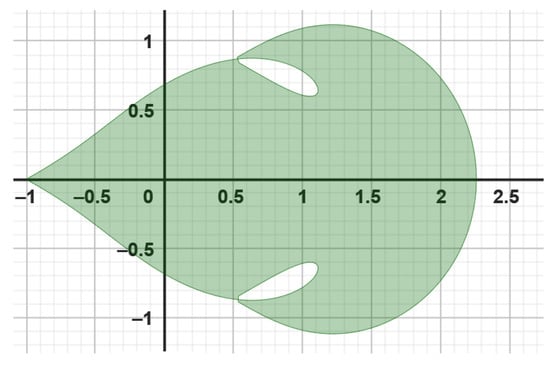
Figure 1.
Leaf-shaped region, displays the image of (in green color) where .
Quantum calculus, or -calculus, does not use the idea of a derivative as the limit of a ratio as the increment tends to zero. Instead, it relies on the -operator, which is crucial for our discussion. This calculus expands the traditional concepts of mathematical analysis by introducing the parameter . For a detailed exploration of this topic, readers are advised to check the comprehensive treatise by Gasper and Rahman [11], which offers in-depth explanations and practical applications of -difference calculus in a variety of disciplines, including number theory, physics, and combinatorics.
Definition 1
([12]). The -bracket represented by is defined explicitly for as follows:
With the useful identity .
Definition 2
([12]). The -difference operator, or -derivative, of a function is defined for by:
Because of its numerous applications in physics, quantum mechanics and mathema tics—particularly in the field of geometric function theory—researchers are still drawn to the study of -calculus. A significant aspect of -calculus is the operator , which is important for the analysis of different classes of analytic functions. In 1990, Ismail et al. [13] made a significant breakthrough by introducing the concept of -extension for starlike functions in the unit disk. This breakthrough opened the door for further investigations in geometric function theory. For example, in [14], Srivastava and his colleagues explored -starlike functions in conic domains and conducted studies on the upper bounds of the Fekete–Szegö functional. Recently, Srivastava provided a comprehensive survey that explains the mathematical foundations and practical applications of -derivative operators, within the context of geometric function theory [15]. For those interested in delving deeper into -calculus and its implications in this field, an abundance of research is at one’s disposal, starting with classical publications [16,17], continuing with studies like [18,19,20] and considering very recent research outcome on the topic like [21,22,23,24,25,26,27,28].
Definition 3
([13]). A function of the form (1) is said to belong to the class if it satisfies the condition given by
t5
In a notable observation made by Khan et al. [29], it becomes apparent that as approaches , the inequality lies in:
Furthermore, it is noteworthy that the closed disk mentioned above pertains solely to the right-half plane. Consequently, the class of -starlike functions undergoes a transformation into the well-known class . Similarly, the relationship in Equation (6) can be expressed as follows (see [18]) using the idea of subordination:
In 2020, Khan et al. [29] used -calculus to establish a new subclass of analytic functions related to a specific leaf-like domain. By applying the principles mentioned earlier and the concept of subordination, they were able to identify unique characteristics of this subclass.
Definition 4
([29]). A function is said to belong to the class if its satisfies the condition given by
where
Remark 2.
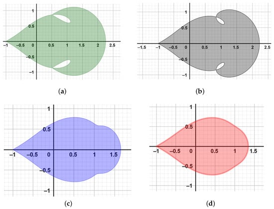
The unit disk is mapped onto a leaf-shaped region via the analytic and univalent function . With regard to the real axis, it is symmetric. The function satisfies and has a positive real part. Figure 2 was generated using Geogebra computer software.
Figure 2.
The figure illustrates the leaf-shaped region , which is bounded and symmetric with respect to the real axis. (a) depicts the image of in green color, with approaches ; (b) displays the image of in gray color, with ; (c) shows the image of in blue color, with ; (d) illustrates the image of in red color as approaches .
The primary objective of this research is to investigate new categories of bi-univalent functions located within the leaf-like domain of the open unit disk . The next section will define the class under examination and provide illustrative examples to facilitate the achievement of this goal. Following that, Section 3 will derive coefficient estimates for the newly defined class, while Section 4 will delve into the evaluation of the Fekete–Szegö functional. Section 5 will then present corollaries that correspond to the given examples, which are generated by the theorems established in the preceding sections.
2. Definition and Examples
We will use the -calculus theory and the previously mentioned subordination principle among analytic functions to give an exact mathematical description of the newly defined class of bi-univalent functions related to a leaf-like domain. The definition of this class is provided below:
Definition 5
A bi-univalent function of the type (1) belongs to the class if it fulfills the following subordinations:
and
where
with and .
Remark 3.
The class is nonempty. There exist two approaches in validating this claim: the analytical approach and the graphical approach.
- Analytically (see [30]): The function defined byis univalent due to being the extremal functions of the class of univalent functions. To show , we proceed as follows.By putting in (9), we have:On the other hand, the Maclaurin series expansion of on the LHS of (11) is as follows:This means that andNow, we check if satisfies the second part of the definition.which impliesNow, substitute (16) into (15), which givesSubstituting and into (16), we havefor the left-hand side of (10). The inverse of follows the same solving process as the L.H.S of (10), since (13) and (14) are equal. That is,Comparing (18) and (19), we deduce that both sides are equal. We conclude that they also satisfy both equations in Definition 5.Now, we can conclude that the extremal function given in (12) shows that our defined class of analytic and bi-univalent function is not empty.
- Geometrically: (see [31]) Let denote the functions given by:To establish the univalence of the function , we commence by assuming that . Our objective is to demonstrate that this assumption implies . We initiate the proof by considering the given condition:Now, let us correct the second equation:This simplifies to:So, indeed, we have shown that , thus proving that is univalent; moreover, with its inverse:By utilizing the notations provided in Equations (9) and (10), we can easily demonstrate through a straightforward calculation thatFurthermore, for every , it follows that , thereby implying that . Hence, we can conclude that , and there exist certain values for the parameters χ and for the identity function such that
We employ the Geogebra computer software (we omit the Geogebra codes for the figures we used throughout the article) to generate the visual representations of the boundary using the functions , , and , as illustrated in Figure 3. This is applicable to various scenarios where the conditions , , and are satisfied. It is worth noting that is a univalent function within . As a consequence, the relationships and are valid. These relationships can be justified by the facts that , , and . Please refer to Figure 3, Figure 4 and Figure 5 for further clarification.
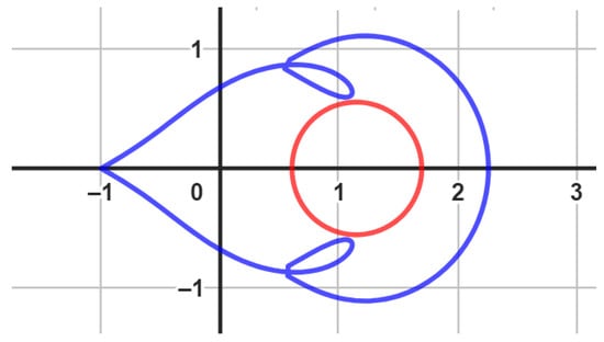
Figure 3.
An image of , (red color) and (blue color) with , , and .
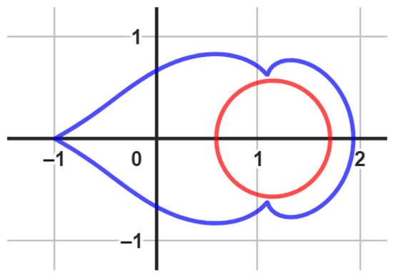
Figure 4.
An image of , (red color) and (blue color) with , , and .
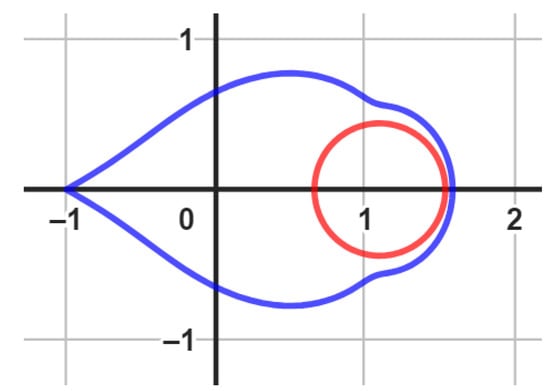
Figure 5.
An image of , (red color) and (blue color) with , , and .
Remark 4.
Special cases:
- Letting , the expression is reduced to , representing the bi-univalent class of functions , provided the following subordination conditions hold:
- If , then the class is reduced to , representing the bi-univalent class of functions , provided the following subordination conditions hold:
- Let and . Then, the class is reduced to , representing the bi-univalent class of functions , provided the following subordination conditions hold:
Up to this moment, there has been a scarcity of academic research on the numerous parameters that influence the functional classification of a leaf-like domain. The fundamental purpose of this work is to examine the initial Taylor–Maclaurin coefficients of functions , as given by Equation (1), which are significant for the class related to a leaf-like domain. Furthermore, we seek to study the estimated value of the Fekete–Szegö functional.
3. The Bounds of the Coefficients within the Class
Initially, the estimates for the coefficients of the class , as defined in Definition 5, are provided.
Theorem 1.
Proof.
If . As per Definition 5, the presence of certain analytic functions and can be established, satisfying the conditions , and , for all . Setting
and
then . From the above relations, we have
and
Also,
and
Substituting the value of from (34), we obtain
Moreover,
Applying (4) for the coefficients and , we obtain
Thus, applying (4), we conclude that
The proof of the theorem has been successfully concluded. □
4. The Fekete–Szegö Functional
Both Fekete and Szegö published their work in 1933, establishing a precise limit for the functional [32]. This limit, known as the classical Fekete–Szegö inequality, was derived using real values of . It is a challenging task to establish precise boundaries for a given function within a compact family of functions , for a real parameter . In this context, the Fekete–Szegö inequality for functions belonging to the class is examined, considering the findings of Zaprawa [33].
Theorem 2.
5. Corollaries
Theorems 1 and 2 generate the corollaries below, which generally correspond to Examples 1–3.
Corollary 1.
If is an element of Σ defined by (1) and belongs to the class , then we can state the following:
and
Corollary 2.
If is an element of Σ defined by (1) and belongs to the class and , then we can state the following:
and
Corollary 3.
If is defined by (1) and belongs to the class , then we can state the following:
6. Conclusions
In this study, we have conducted an investigation on coefficient problems related to recently defined subclasses of bi-univalent functions in given in Definition 5. The investigated subclasses are , , , and . We have computed the Taylor–Maclaurin coefficients and , along with estimates for the Fekete–Szegö functional problem, for functions belonging to each of these bi-univalent function classes.
In future research, the exploration of upper bounds for the Zaclman conjecture and the investigation of Hankel determinants of orders two and three within the aforementioned subclasses show potential for new avenues of research and exploration.
Author Contributions
Conceptualization, A.A. and G.I.O.; Methodology, A.A. and G.I.O.; Software, A.A. and G.I.O.; Validation, A.A. and G.I.O.; Formal analysis, A.A. and G.I.O.; Investigation, A.A. and G.I.O.; Resources, A.A. and G.I.O.; Data curation, A.A. and G.I.O.; Writing—original draft, A.A. and G.I.O.; Writing—review & editing, A.A. and G.I.O.; Visualization, A.A. and G.I.O.; Supervision, A.A.; Project administration, A.A.; Funding acquisition, G.I.O. All authors have read and agreed to the published version of the manuscript.
Funding
This research received no external funding.
Data Availability Statement
No data were used to support this study.
Acknowledgments
The first author expresses their gratitude to Philadelphia University-Jordan for supporting this work, emphasizing non-financial support in providing necessary resources.
Conflicts of Interest
The authors declare no conflict of interest.
References
- Miller, S.S. Differential inequalities and Carathéodory functions. Bull. Am. Math. Soc. 1975, 81, 79–81. [Google Scholar] [CrossRef]
- Duren, P.L. Univalent Functions; Grundlehren der Mathematischen Wissenschaften, Band 259; Springer: New York, NY, USA; Berlin/Heidelberg, Germany; Tokyo, Japan, 1983. [Google Scholar]
- Ma, W.; Minda, D. A unified treatment of some special classes of univalent functions. In Proceedings of the Complex Analysis, Tianjin, China, 16–20 March 1992; pp. 157–169. [Google Scholar]
- Sokół, J.; Stankiewicz, J. Radius of convexity of some subclasses of strongly starlike functions. Zeszyty Nauk. Politech. Rzeszowskiej Mat. 1996, 19, 101–105. [Google Scholar]
- Raina, R.K.; Sokól, R.K. On Coefficient estimates for a certain class of starlike functions. Hacettepe J. Math. Statist. 2015, 44, 1427–1433. [Google Scholar] [CrossRef]
- Priya, M.H.; Sharma, R.B. On a class of bounded turning functions subordinate to a leaf-like domain. J. Phys. Conf. Ser. 2018, 1000, 012056. [Google Scholar] [CrossRef]
- Rath, B.; Kumar, K.S.; Krishna, D.V.; Lecko, A. The sharp bound of the third Hankel determinant for starlike functions of order 1/2. Complex Anal. Oper. Theory 2022, 16, 1–8. [Google Scholar] [CrossRef]
- Mahmood, S.; Srivastava, H.M.; Khan, N.; Ahmad, Q.Z.; Khan, B.; Ali, I. Upper bound of the third Hankel determinant for a subclass of q-starlike functions. Symmetry 2019, 11, 347. [Google Scholar] [CrossRef]
- Ullah, K.; Srivastava, H.M.; Rafiq, A.; Arif, M.; Arjika, S. A study of sharp coefficient bounds for a new subfamily of starlike functions. J. Inequal. Appl. 2021, 2021, 194. [Google Scholar] [CrossRef]
- Shi, L.; Shutaywi, M.; Alreshidi, N.; Arif, M.; Ghufran, S.M. The sharp bounds of the third-order Hankel determinant for certain analytic functions associated with an eight-shaped domain. Fractal Fract. 2022, 6, 223. [Google Scholar] [CrossRef]
- Gasper, G.; Rahman, M. Basic Hypergeometric Series, 2nd ed.; Encyclopedia of Mathematics and Its Applications; Cambridge University Press: Cambridge, MA, USA, 2004; Volume 96. [Google Scholar]
- Alsoboh, A.; Amourah, A.; Sakar, F.M.; Breaz, D. New Subfamily of Bi-starlike and Bi-convex Functions Defined by the q-Janowski Function. Preprints 2023, 2023061002. [Google Scholar] [CrossRef]
- Ismail, M.E.; Merkes, E.; Styer, D. A generalization of starlike functions. Complex Var. Theory Appl. 1990, 14, 77–84. [Google Scholar] [CrossRef]
- Srivastava, H.M.; Khan, B.; Khan, N.; Ahmad, Q.Z.; Tahir, M. A generalized conic domain and its applications to certain subclasses of analytic functions. Rocky Mt. J. Math. 2019, 49, 2325–2346. [Google Scholar] [CrossRef]
- Srivastava, H.M. Operators of basic (or q-) calculus and fractional q-calculus and their applications in geometric function theory of complex analysis. Iran. J. Sci. Technol. Trans. A Sci. 2020, 44, 327–344. [Google Scholar] [CrossRef]
- Al-Salam, W.A. Some fractional q-integrals and q-derivatives. Proc. Edinburgh Math. Soc. 1966, 15, 135–140. [Google Scholar] [CrossRef]
- Agarwal, R.P. Certain fractional q-integrals and q-derivatives. Proc. Cambridge Philos. 1969, 66, 365–370. [Google Scholar] [CrossRef]
- Uçar, H.E.Ö. Coefficient inequality for q-starlike functions. App. Math. Comput. 2016, 276, 122–126. [Google Scholar] [CrossRef]
- Aldweby, H.; Darus, M. Some subordination results on q-analogue of Ruscheweyh differential operator. Abstr. Appl. Anal. 2014, 2014, 958563. [Google Scholar] [CrossRef]
- Aldweby, H.; Darus, M. On a subclass of bi-univalent functions associated with the q-derivative operator. J. Math. Comput. Sci. 2019, 19, 58–64. [Google Scholar] [CrossRef]
- Ahuja, O.; Bohra, N.; Cetinkaya, A.; Kumar, S. Univalent functions associated with the symmetric points and cardioid-shaped domain involving (p,q)-calculus. Kyungpook Math. J. 2021, 61, 75–98. [Google Scholar]
- Alb Lupaş, A.; Oros, G.I. Sandwich-type results regarding Riemann-Liouville fractional integral of q-hypergeometric function. Demonstr. Math. 2023, 56, 20220186. [Google Scholar] [CrossRef]
- Ali, E.E.; Oros, G.I.; Albalahi, A.M. Differential subordination and superordination studies involving symmetric functions using a q-analogue multiplier operator. AIMS Math. 2023, 8, 27924–27946. [Google Scholar] [CrossRef]
- Andrei, L.; Căuș, V.A. Subordinations Results on a q-Derivative Differential Operator. Mathematics 2024, 12, 208. [Google Scholar] [CrossRef]
- Khan, M.F.; AbaOud, M. New Applications of Fractional q-Calculus Operator for a New Subclass of q-Starlike Functions Related with the Cardioid Domain. Fractal Fract. 2024, 8, 71. [Google Scholar] [CrossRef]
- Alsoboh, A.; Amourah, A.; Darus, M.; Rudder, C.A. Studying the Harmonic Functions Associated with Quantum Calculus. Mathematics 2023, 11, 2220. [Google Scholar] [CrossRef]
- Alsoboh, A.; Amourah, A.; Darus, M.; Rudder, C.A. Investigating New Subclasses of Bi-Univalent Functions Associated with q-Pascal Distribution Series Using the Subordination Principle. Symmetry 2023, 15, 1109. [Google Scholar] [CrossRef]
- Alsoboh, A.; Amourah, A.; Sakar, F.M.; Ogilat, O.; Gharib, G.M.; Zomot, N. Coefficient Estimation Utilizing the Faber Polynomial for a Subfamily of Bi-Univalent Functions. Axioms 2023, 12, 512. [Google Scholar] [CrossRef]
- Khan, B.; Srivastava, H.M.; Khan, N.; Darus, M.; Tahir, M.; Ahmad, Q.Z. Coefficient Estimates for a Subclass of Analytic Functions Associated with a Certain Leaf-Like Domain. Mathematics 2020, 8, 1334. [Google Scholar] [CrossRef]
- Shaba, T.G.; Araci, S.; Ro, J.-S.; Tchier, F.; Adebesin, B.O.; Zainab, S. Coefficient Inequalities of q-Bi-Univalent Mappings Associated with q-Hyperbolic Tangent Function. Fractal Fract. 2023, 7, 675. [Google Scholar] [CrossRef]
- Analouei Adegani, E.; Jafari, M.; Bulboacă, T.; Zaprawa, P. Coefficient Bounds for Some Families of Bi-Univalent Functions with Missing Coefficients. Axioms 2023, 12, 1071. [Google Scholar] [CrossRef]
- Fekete, M.; Szegö, G. Eine Bemerkung über ungerade schlichte Funktionen. J. Lond. Math. Soc. 1933, 1, 85–89. [Google Scholar] [CrossRef]
- Zaprawa, P. On the Fekete-Szegö problem for classes of bi-univalent functions. Bull. Belg. Math. Soc. Simon Stevin 2014, 21, 169–178. [Google Scholar] [CrossRef]
Disclaimer/Publisher’s Note: The statements, opinions and data contained in all publications are solely those of the individual author(s) and contributor(s) and not of MDPI and/or the editor(s). MDPI and/or the editor(s) disclaim responsibility for any injury to people or property resulting from any ideas, methods, instructions or products referred to in the content. |
© 2024 by the authors. Licensee MDPI, Basel, Switzerland. This article is an open access article distributed under the terms and conditions of the Creative Commons Attribution (CC BY) license (https://creativecommons.org/licenses/by/4.0/).