Article

Analysis of a Two-Stage Tandem Queuing System with Priority and Clearing Service in the Second Stage

School of Mathematics and Statistics, Nanjing University of Science and Technology, Nanjing 210094, China
*
Author to whom correspondence should be addressed.
Mathematics 2024, 12(10), 1500; https://doi.org/10.3390/math12101500
Submission received: 28 April 2024 / Revised: 8 May 2024 / Accepted: 9 May 2024 / Published: 11 May 2024
(This article belongs to the Special Issue Queueing Systems Models and Their Applications)

Abstract

:
This paper considers a two-stage tandem queuing system with ordinary customers and priority customers. Upon arrival, ordinary customers are individually served in the first stage, then move to the second stage and receive clearing service. Priority customers can bypass the first stage and proceed directly to the second stage for clearing service. The second stage has N service seats. All customers currently in the second stage are served simultaneously (i.e., clearing service). Once there are N customers in the second stage, the first stage will be blocked, and newly arriving priority customers will balk and leave without joining. We first formulate a two-dimensional Markov chain to analyze this queuing system and derive the stability condition. Subsequently, the stationary distribution of the system is derived using the matrix-analytic method and spectral expansion technique. Furthermore, analytical expressions for the mean queue length, mean sojourn time, and other performance measures are presented. Finally, some numerical examples are provided to illustrate the effects of various parameters, offering valuable insights for designing such two-stage tandem queuing systems.

1. Introduction

This study investigates a two-stage tandem queuing system with two types of customers: ordinary and priority customers. Upon arrival, an ordinary customer enters the first stage and receives a single service. After completing this service, he/she moves to the second stage and receives a clearing service. However, an arriving priority customer can bypass the first queue and directly join the second stage to receive the clearing service. The second stage has a maximum capacity of N service seats. Priority customers can only enter the system if there are fewer than N customers already in the second stage upon their arrival; otherwise, they will leave without joining the system. Ordinary customers always enter the first stage and wait for service. Once the number of customers being served simultaneously in the second stage reaches the threshold N, the first stage stops providing service, and customers in the first stage are blocked. Until a service seat becomes available in the second stage, the service in the first stage resumes.
The analyzed two-stage tandem queuing system with priority is inspired by public transportation systems. When taking public transport (e.g., buses, subways, trains, or planes), passengers holding prepaid cards, ride cards, or those who buy tickets online are given priority. They can skip the physical queue at the ticket office and directly access the waiting room. As shown in Figure 1, ordinary passengers initially proceed to the ticket office, join a queue to purchase tickets, and then move to the waiting room to prepare for boarding. Priority passengers who have ride cards or buy tickets online, on the other hand, enter the waiting room immediately. Once the scheduled departure time arrives, all passengers in the waiting room, including both ordinary and priority passengers, board the designated vehicle and leave the station together. The seating capacity in cars, trains, or flights is predetermined and finite. As soon as all seats are filled, the ticket office stops selling tickets, and online ticket purchases are also suspended. This means that when the number of customers in the second stage reaches the threshold, ordinary customers in the first stage are all blocked, and priority customers balk.
Examples of the two-stage tandem service system with priority can also be seen in various sectors, such as amusement parks and production systems. In amusement parks, visitors go through a ticket check before entering the facilities. These facilities have limited capacity, and the ticket check process stops when all seats are occupied. After completing the ticket check, a group of visitors enters the facility together and experiences the services simultaneously. However, certain rides may be popular, making it challenging to enjoy them in a short amount of time. To address this, amusement parks often provide paid fast-pass tickets (e.g., Universal Studios’ Express Pass and Disney’s Lightning Lane). Holders of fast-pass tickets can skip the regular ticket check queue and enter the facility directly. However, if the seats are already full, those with fast-pass tickets cannot enter the facility and must wait in the fast-pass queue.
Another example is a production system: The first stage involves the factory receiving and organizing orders, while the second stage entails manufacturing products for those orders. Each batch of products can fulfill a set number of orders. Rush orders receive higher priority and are processed immediately without queuing in the first stage. The output of a factory is capped within a production cycle. When the quantity reaches the maximum, the factory ceases to accept rush orders and stops the arrangement of incoming orders.
A tandem queue is a queuing system organized in the series queue in which service facilities provide services in sequence [1,2,3,4]. Since Jackson [5] introduced the analytical frameworks of interconnected queues, tandem queuing systems have been extensively analyzed due to their applicability across various sectors (such as communication, transportation, manufacturing, networks) [6,7,8]. Neuts [9] studied a two-stage tandem system using an embedded semi-Markov process, where the arrival process of customers follows a Poisson process, the service time at the first stage follows a general distribution, and the service time at the second stage follows an exponential distribution, with a finite buffer between the two stages. Moreover, Neuts [10] proposed the matrix-analytic technique to study queuing systems, which helps us to handle various complex tandem queues effectively. In this paper, we employ this method to compute the steady-state distribution of the considered system.
Yang et al. [11] analyzed a two-stage tandem queuing system featuring a single service in the first stage and a batch service in the second stage, both provided by a single switched server under N policy. Recently, Nazarov et al. [12] studied a queuing network with two servers in series and two infinite orbits using the asymptotic analysis method. Dudin, Dudina, and Dudin [13] considered a dual queuing model with multiple servers in the second stage. In their model, customers are served individually in the first stage, while services are rendered to groups with variable service time based on group size in the second stage. To the best of our knowledge, there has been no research study on such a two-stage tandem queuing system with a single service at stage one and a clearing service at stage two, where priority customers can skip stage one and join stage two immediately. The clearing service can be regarded as a flexible batch service, as it also processes multiple customers simultaneously but without limiting the batch size. This service mode tends to clear all customers in the queue at once, which is different from the fixed batch size characteristic of batch service.
In a priority queue system, customers are served based on the order of their priority. There are two types of priority in queuing systems: preemptive [14,15] and non-preemptive [16,17,18]. Preemptive priority occurs when a high-priority customer arrives, and the server halts service to a lower-priority customer to serve the higher-priority one immediately. Conversely, for non-preemptive priority, although newly arrived high-priority customers cannot interrupt ongoing service to lower-priority customers, they are placed ahead in the queue, or only high-priority customers are allowed to enter the system in some cases. Liu and Zhao [19] studied an M 1 , M 2 / G 1 , G 2 / 1 queuing model with non-preemptive priority, analyzing the tail asymptotic properties of steady-state queue length. Lee et al. [20] considered the single server finite queue with non-preemptive priority and phase-type distributed service time. A two-stage tandem queue consisting of infinite servers in the first stage and finite servers in the second stage was proposed by Kim and Dudin [21]. When the number of servers occupied in the second stage reaches the threshold, non-priority customers cannot enter the system upon arrival. On the other side, Atencia [22] analyzed a discrete-time queuing model with general distributed service time and preemptive priority service, while Xie et al. [23] investigated an M / M / 1 queuing system where preemptive service allows low-priority customers to be upgraded to high-priority. More recently, Xu, Liu, and Wu [24] considered an M / G / 1 retrial queue with preemptive priority operating on a Bernoulli schedule, where a new arrival either immediately displaces the current customer being served with a probability α or joins the retrial orbit with a probability 1 α . Chamberlain and Starobinski [25] studied a single server queue with preemptive-resume service and general distributed service time, customer equilibrium joining strategies, and social welfare under the unobservable scenario are presented. In this paper, we study a two-stage tandem service system with priority. In contrast to the previous traditional pure preemptive service or non-preemptive service, we consider the customer who has priority to bypass the single service at stage one and immediately join stage two for clearing service.
In this study, we model the interested service system as a two-stage tandem queuing model with two types of customers, where stage one provides a single service while stage two offers a clearing service. Our focus lies on the steady-state performance analysis of such service systems. To achieve this, we investigated the system’s stability condition and steady-state distribution, which are crucial for understanding its performance. Then, some system performance metrics for given parameters can be calculated using the provided computation algorithm. The main contributions and innovations of this paper are summarized as follows:
1.
We propose a novel tandem queuing model consisting of a single service at stage one and a clearing service at stage two that is commonly found in real life. In the model, we also consider customers with priority to bypass stage one and directly access stage two for service, which is more in line with the practical situation.
2.
We formulate the studied system as a two-dimensional Markov chain and derive the stationary distribution using the matrix-analytic and spectral expansion methods. Our theoretical results may be useful for solving problems in similar service systems.
3.
We conduct sensitivity analysis of various parameters on system performance characteristics, providing a theoretical foundation and practical guidance for service system design and optimization.
The rest of this paper is organized as follows. First, we describe the queuing model and how it was formulated in Section 2. We then analyze the system stability condition in Section 3. In Section 4, we provide the system stationary probability distribution and expected sojourn time of customers. Furthermore, some essential performance measures are obtained in Section 5. In Section 6, we present the sensitivity analysis of various system parameters. Finally, the conclusion is given in Section 7.

2. Queuing Model and Its Formulation

We are interested in a two-stage tandem queuing system that includes ordinary and priority customers, where stage one provides a single service while stage two provides a clearing service. The schematic diagram of the queuing service system is illustrated in Figure 2.
The system operates with two separate queues, and each queue is managed independently by dedicated servers. Queue 1 and queue 2 represent the queues at stage one and stage two (including customers being serviced), respectively. The studied service system caters to two types of customers: (1) Ordinary customers, who first enter queue 1 and receive a single service at stage one, then move to queue 2 for clearing service at stage two; (2) Priority customers, who bypass the first stage and directly enter queue 2 for service at stage two. The detailed queuing model is explained below:
  • The capacity of queue 1 is infinite, while queue 2 has N spots.
  • Ordinary and priority customers arrive at the system according to two independent Poisson processes with arrival rates λ 1 and λ 2 , respectively.
  • Upon the arrival of a priority customer, if the number of customers in the second stage reaches the threshold N, the customer will balk (leaves without joining the system), i.e., a priority customer enters the system only when the number of customers at stage two is fewer than N upon his/her arrival.
  • Ordinary customers are served individually (single service) in the first stage based on the First-Come-First-Served (FCFS) discipline. All customers are served together (clearing service) in the second stage. There are N customers who are being served in the second stage at most. The single service time and clearing service time are independent and exponentially distributed with parameters μ 1 and μ 2 , respectively.
  • If the number of customers in the second stage is fewer than N, any ordinary customer who finished their service at stage one will immediately move to stage two and receive a clearing service. However, if the queue length of the second stage reaches the capacity threshold N, the first stage and ordinary customers in the first stage will be blocked. In this case, the first stage stops providing service even if there are some customers in the first stage. The service in the first stage will be resumed only when some spots are available in the second stage.
Let q 1 ( t ) and q 2 ( t ) be the number of customers in queue 1 and queue 2 at time t (including the customers being serviced), respectively. Then, the queuing model is formulated as a two-dimensional continuous-time Markov chain { ( q 1 ( t ) , q 2 ( t ) ) , t 0 } with state space
Ω = { ( 0 , 0 ) , ( 0 , 1 ) , , ( 0 , N ) ; ( 1 , 0 ) , , ( 1 , N ) ; ; ( n , 0 ) , ( n , 1 ) , , ( n , N ) ; } .
When q 2 = N , the first stage stops serving customers, and the first stage is blocked, as are the customers at stage one. Please note that this case does not contribute to the probability that the first stage is busy (working). If all system parameters are positive, it is clear that the continuous-time Markov chain { ( q 1 ( t ) , q 2 ( t ) ) , t 0 } is irreducible.
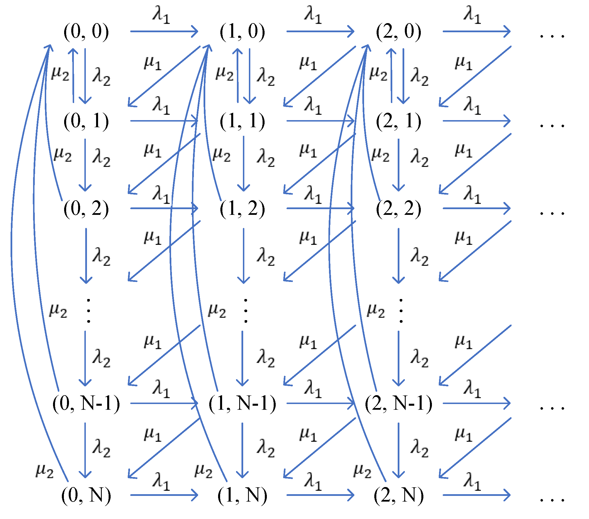
Let q ( ( q 1 , q 2 ) , ( y 1 , y 2 ) ) be the transition rate from state ( q 1 , q 2 ) to state ( y 1 , y 2 ) , then the infinitesimal generator of the Markov chain is Q = q ( ( q 1 , q 2 ) , ( y 1 , y 2 ) ) , ( q 1 , q 2 ) Ω , ( y 1 , y 2 ) Ω . The transition rate diagram for this two-stage tandem service system is depicted in Figure 3. For ( q 1 , q 2 ) Ω , the one-stop transition rates are given by
q ( q 1 , q 2 ) , ( q 1 + 1 , q 2 ) = λ 1 , q ( q 1 , q 2 ) , ( q 1 , q 2 + 1 ) = λ 2 , q ( q 1 , q 2 ) , ( q 1 1 , q 2 + 1 ) = μ 1 , ( q 1 > 0 , q 2 < N ) , q ( q 1 , q 2 ) , ( q 1 , 0 ) = μ 2 , ( q 2 > 0 ) .

3. Stability Condition

This section analyzes the system stability condition based on the matrix-geometric solution in [26]. The infinitesimal generator of the above continuous-time Markov chain { ( q 1 ( t ) , q 2 ( t ) ) , t 0 } can be written as the block-partitioned form:
Q = B A 0 0 0 0 A 2 A 1 A 0 0 0 0 A 2 A 1 A 0 0 ,
the matrices B , A 0 , A 1 , and A 2 are both ( N + 1 ) -dimensional square matrices with elements, where
B = ( λ 1 + λ 2 ) λ 2 μ 2 ( λ 1 + λ 2 + μ 2 ) λ 2 μ 2 ( λ 1 + λ 2 + μ 2 ) λ 2 μ 2 ( λ 1 + μ 2 ) ,
A 0 = λ 1 λ 1 λ 1 , A 2 = 0 μ 1 0 μ 1 0 ,
A 1 = ( λ 1 + λ 2 + μ 1 ) λ 2 μ 2 ( λ 1 + λ 2 + μ 1 + μ 2 ) λ 2 μ 2 ( λ 1 + λ 2 + μ 1 + μ 2 ) λ 2 μ 2 ( λ 1 + μ 2 ) .
Obviously, according to the characteristics of matrix Q , we can know that the Markov chain { ( q 1 ( t ) , q 2 ( t ) ) , t 0 } is a quasi-birth-and-death ( Q B D ) process.
Theorem 1. 
The considered two-stage tandem queuing system is stable if and only if
ρ = λ 1 μ 1 + λ 2 + μ 1 λ 2 + μ 1 + μ 2 N < 1 .
Proof. 
According to the mean drift result in [10], the system would be stable, and the stationary distributions exist if and only if
XA 0 e < XA 2 e ,
where e is a ( N + 1 ) -dimensional column vector with all elements are equal to 1, X = ( X 1 , X 2 , , X N + 1 ) is the invariant probability vector of A = A 0 + A 1 + A 2 , and
A = 1 2 N N + 1 ( λ 2 + μ 1 ) λ 2 + μ 1 μ 2 ( λ 2 + μ 1 + μ 2 ) λ 2 + μ 1 μ 2 ( λ 2 + μ 1 + μ 2 ) λ 2 + μ 1 μ 2 μ 2 .
Then, we have the following balance equations
XA = 0 ,
Xe = 1 .
Expanding Equation (1) yields the following equations
( λ 2 + μ 1 ) X 1 + μ 2 n = 2 N + 1 X n = 0 , ( λ 2 + μ 1 ) X n 1 ( λ 2 + μ 1 + μ 2 ) X n = 0 , 2 n N , ( λ 2 + μ 1 ) X N μ 2 X N + 1 = 0 ,
which, by recursive iteration, yield
X n = λ 2 + μ 1 λ 2 + μ 1 + μ 2 n 1 X 1 , 1 n N , λ 2 + μ 1 μ 2 λ 2 + μ 1 λ 2 + μ 1 + μ 2 N 1 X 1 , n = N + 1 .
Substituting (3) into (2) results in
X N + 1 = λ 2 + μ 1 λ 2 + μ 1 + μ 2 N .
The stability condition XA 0 e < XA 2 e can be rewritten as
λ 1 < μ 1 ( 1 X N + 1 ) .
By substituting (4) into (5), we obtain the stability condition of the studied system
λ 1 < μ 1 1 λ 2 + μ 1 λ 2 + μ 1 + μ 2 N .
After transforming the above equation, we have
ρ = λ 1 μ 1 + λ 2 + μ 1 λ 2 + μ 1 + μ 2 N < 1 .
Thus, the proof is completed.    □
Remark 1. 
Due to the finite capacity of the second stage, achieving a steady-state system necessitates that the arrival rate of ordinary customers at the first stage remains below the actual service rate of the first stage. If the two queues are independent, the service rate of the first stage is μ 1 . However, as the two queues are tandem in series, the departure from the first stage is constrained by the capacity of the second stage. Please note that the term λ 2 + μ 1 λ 2 + μ 1 + μ 2 N represents the probability that the second stage queue reaches its maximum capacity N (i.e., the probability that the first stage is blocked). Therefore, μ 1 1 λ 2 + μ 1 λ 2 + μ 1 + μ 2 N means the effective service rate of the first stage. Thus, the stability condition ensures a balance between the arrival rate of ordinary customers and the ability of this system to accept and process them, considering the limitations imposed by the finite capacity of the second stage and priority customers, therefore ensuring the maintenance of stable system operation.

4. Steady-State Analysis

Under the condition of system stability, this section will determine the stationary distribution and calculate the sojourn times of customers within the system.

4.1. Stationary Probability Distribution

This section will calculate the stationary probabilities for the queuing model under study using matrix-analytic and spectral expansion methods. We first define the steady-state joint probabilities of the Markov chain under consideration as:
π i , j = lim t P { q 1 ( t ) = i , q 2 ( t ) = j ) } , i 0 , 0 j N . π i = ( π i , 0 , π i , 1 , π i , 2 , , π i , N ) , i 0 , π = ( π 0 , π 1 , π 2 , ) .
When the stability condition ρ < 1 is satisfied, the steady-state system has the following Chapman-Kolmogorov equations based on the above definitions:
( λ 1 + λ 2 ) π 0 , 0 = μ 2 j = 1 N π 0 , j , ( λ 1 + λ 2 + μ 2 ) π 0 , j = λ 2 π 0 , j 1 + μ 1 π 1 , j 1 , 1 j N 1 ,
( λ 1 + μ 2 ) π 0 , N = λ 2 π 0 , N 1 + μ 1 π 1 , N 1 , ( λ 1 + λ 2 + μ 1 ) π i , 0 = λ 1 π i 1 , 0 + μ 2 j = 1 N π i , j , i 1 , ( λ 1 + λ 2 + μ 1 + μ 2 ) π i , j = λ 1 π i 1 , j + λ 2 π i , j 1 + μ 1 π i + 1 , j 1 , i 1 , 1 j N 1 , ( λ 1 + μ 2 ) π i , N = λ 1 π i 1 , N + λ 2 π i , N 1 + μ 1 π i + 1 , N 1 , i 1 .
The normalization equation is
i = 0 ( π i , 0 + π i , 1 + π i , 2 + + π i , N ) = 1 .
From π Q = 0 , we have
π 0 B + π 1 A 2 = 0 ,
π i 1 A 0 + π i A 1 + π i + 1 A 2 = 0 , i 1 .
Employing the matrix-geometric method described in Neuts [10], we establish that
π i = π 0 R i , i 0 ,
where R is the minimal nonnegative solution to the matrix quadratic equation
A 0 + RA 1 + R 2 A 2 = 0 .
The matrices A 0 , A 1 , and A 2 have complex forms, making direct analytical expressions for the rate matrix R challenging. The rate matrix R is typically calculated using the Gauss-Seidel iterative method, starting with
R 0 = 0 ,
and updating with
R i + 1 = R i 2 A 2 + A 0 A 1 1 , i 0 .
The specifics of this approximation technique are outlined in Algorithm 1.    
Algorithm 1: Pseudo code for deriving the rate matrix R .
Input: Tolerance ε > 0 , n = 1 , matrix A 0 , A 1 , and A 2 .
Output: Rate matrix R .
Step 1: Set R 0 = 0 .
Step 2:  R 1 = R 0 2 A 2 + A 0 A 1 1 .
Step 3: While  R n R n 1 > ε   do
                   n = n + 1 ;
                   R n = R n 1 2 A 2 + A 0 A 1 1 .
         End while
Step 4:  R = R n .
By substituting (9) into the first matrix balance Equation (7), it is obtained
π 0 B + RA 2 = 0 ,
and substituting (9) in the normalizing equation results in
i = 0 π 0 R i e = π 0 i R 1 e = 1 ,
where I is a ( N + 1 ) × ( N + 1 ) identity matrix (i.e., all its diagonal elements are 1 and everywhere else is 0), and e is a ( N + 1 ) -dimensional column vector with all elements are 1. Then π 0 can be obtained by solving Equations (10) and (11), and starting from π 0 , the system’s stationary probability vector ( π 0 , π 1 , π 2 , ) can be calculated using π i = π 0 R i .
Based on the analysis presented, we propose the following theorem.
Theorem 2. 
When the stability condition ρ < 1 is satisfied, the steady-state probabilities of the system can be expressed as
π i = π 0 R i , i 0 ,
where π 0 is determined by the unique solution to the equations
π 0 B + RA 2 = 0 , π 0 i R 1 e = 1 .
Let E [ L 1 ] be the expected queue length of the first stage (including the customer being serviced), and let E [ L 2 ] be the expected queue length of the second stage. Note that all customers in the first stage are ordinary customers. Then, the expected number of ordinary customers in the first stage is given by
E [ L 1 ] = i = 0 j = 0 N i π i , j = i = 0 i π i e = i = 0 i π 0 R i e = π 0 i = 0 i R i e = π 0 R ( I R ) 2 e .
For v = ( 0 , 1 , 2 , , N 1 , N ) T , the expected queue length of the second stage is given by
E [ L 2 ] = i = 0 j = 0 N j π i , j = i = 0 π i v = π 0 i = 0 R i v = π 0 I R 1 v .
Thus, the expected number of customers in the system is given by
E [ L ] = E [ L 1 ] + E [ L 2 ] = π 0 R ( I R ) 2 e + I R 1 v .
As an alternative to the matrix-analytic method, we next use another technique (spectral expansion method) to derive the steady-state probability distribution of the studied two-stage tandem queuing system with priority, which is favorable in some cases [26,27].
The characteristic matrix polynomial of equation π i 1 A 0 + π i A 1 + π i + 1 A 2 = 0 , ( i 1 ) has the following structure:
Q ( x ) = A 0 + A 1 x + A 2 x 2 = 1 2 N N + 1 d 1 ( x ) d 4 ( x ) μ 2 x d 2 ( x ) d 4 ( x ) μ 2 x d 2 ( x ) d 4 ( x ) μ 2 x d 3 ( x ) ,
where
d 1 ( x ) = λ 1 ( λ 1 + λ 2 + μ 1 ) x , d 2 ( x ) = λ 1 ( λ 1 + λ 2 + μ 1 + μ 2 ) x , d 3 ( x ) = λ 1 ( λ 1 + μ 2 ) x , d 4 ( x ) = λ 2 x + μ 1 x 2 .
According to Proposition 2 in [26], if the system is stable, the characteristic polynomial Q ( x ) contains N + 1 eigenvalues inside the unit circle. Consequently, the steady-state probabilities can be reformulated as follows:
π i = k = 1 N + 1 a k ν k i φ k , i 0 ,
where a k is the coefficient determined through balance equations, and the normalization condition, ν k represents the eigenvalues within the unit circle, and φ k are the corresponding left eigenvectors. A pair of ( ν k , φ k ) associated with Q ( x ) satisfy
φ k Q ( ν k ) = 0 , det ( Q ( ν k ) ) = 0 .
Define ν 1 , ν 2 , ⋯, ν N + 1 as the eigenvalues of Q ( x ) inside the unit circle, with the corresponding eigenvectors φ k = ( φ k , 1 , φ k , 2 , , φ k , N + 1 ) . From the equation φ k Q ( ν k ) = 0 , we have
φ k , 1 d 1 ( ν k ) + j = 2 N + 1 φ k , j μ 2 ν k = 0 ,
φ k , j ( λ 2 ν k + μ 1 ν k 2 ) + φ k , j + 1 d 2 ( ν k ) = 0 , j = 1 , 2 , , N 1 ,
φ k , N ( λ 2 ν k + μ 1 ν k 2 ) + φ k , N + 1 d 3 ( ν k ) = 0 .
Letting φ k , 1 = 1 , after some calculation, it can be obtained that
φ k , j = λ 2 ν k + μ 1 ν k 2 d 2 ( ν k ) j 1 , j = 1 , 2 , , N , λ 2 ν k + μ 1 ν k 2 d 3 ( ν k ) λ 2 ν k + μ 1 ν k 2 d 2 ( ν k ) N 1 , j = N + 1 .
Therefore, the coefficients a k are computed using the balance equations and normalization condition based on the derived eigenvalues and corresponding left eigenvectors:
k = 1 N + 1 a k ( λ 1 + λ 2 ) φ k , 1 μ 2 j = 2 N + 1 φ k , j = 0 ,
k = 1 N + 1 a k ( λ 1 + λ 2 + μ 2 ) φ k , j λ 2 φ k , j 1 μ 1 ν k φ k , j 1 = 0 , j = 2 , 3 , , N ,
k = 1 N + 1 a k ( λ 1 + μ 2 ) φ k , N + 1 λ 2 φ k , N μ 1 ν k φ k , N = 0 ,
k = 1 N + 1 a k 1 1 ν k φ k e = 1 .
Note that the system comprises N + 1 independent linear equations, which facilitate the determination of the N + 1 unknown coefficients a 1 , a 2 , ⋯, a N + 1 . Once these coefficients are derived, explicit expressions for the stationary probabilities can be obtained.

4.2. Sojourn Time of a Customer in the System

Define W as the expected sojourn time of an ordinary customer in the system and T as the expected sojourn time of a priority customer in the system. For every priority customer, the time spent in the second stage is equivalent to their total time in the system. Since customers in the second stage are served simultaneously, the expected residual service time in the second stage corresponds to the average time a customer spends in this stage. Additionally, the clearing service time follows an exponential distribution, which is characterized by its memoryless property. Thus, the expected sojourn time of a priority customer in the system is
T = 1 μ 2 .
Define W i , j ( i 0 , 0 j N ) as the conditional expected sojourn time of an ordinary customer, assuming there are i customers in the first stage and j customers in the second stage when the ordinary customer arrives. In the following, Theorem 3 provides the specific expression for computing the expected sojourn time of ordinary customers W i , j .
Theorem 3. 
If the stability condition ρ < 1 is satisfied, and the system is in state ( i , j ) when an ordinary customer arrives, the expected sojourn time of the ordinary customer in the system can be given as follows,
W i , 0 = μ 2 f i , N 1 μ 2 ( 1 h N ) , W i , j = f i , j + h j W i , 0 , 1 j N ,
where
h j = μ 1 + λ 2 λ 2 , j = 1 , ( μ 1 + λ 2 + μ 2 ) h j 1 μ 2 λ 2 , 2 j N ,
f i , j = μ 1 + μ 2 λ 2 μ 2 , i = 0 , j = 1 , f 0 , 1 + μ 1 + λ 2 + μ 2 λ 2 f 0 , j 1 , i = 0 , 2 j N , 1 + μ 1 W i 1 , 1 λ 2 , i 1 , j = 1 , 1 + μ 1 W i 1 , j λ 2 + μ 1 + λ 2 + μ 2 λ 2 f i , j 1 , i 1 , 2 j N .
Proof 
Case (a)  i = 0 . There are no customers in the first stage upon the arrival of a new ordinary customer. By conditioning on the next future event (first-step analysis) and using the strong Markov property, we have
W 0 , 0 = 1 μ 1 + λ 2 + μ 1 μ 1 + λ 2 1 μ 2 + λ 2 μ 1 + λ 2 W 0 , 1 ,
W 0 , j = 1 μ 1 + λ 2 + μ 2 + μ 1 μ 1 + λ 2 + μ 2 1 μ 2 + λ 2 μ 1 + λ 2 + μ 2 W 0 , j + 1 + μ 2 μ 1 + λ 2 + μ 2 W 0 , 0 , 1 j N 1 ,
W 0 , N = 1 μ 2 + W 0 , 0 .
From (12) and (13), we can obtain
W 0 , 1 = μ 1 + μ 2 λ 2 μ 2 + μ 1 + λ 2 λ 2 W 0 , 0 ,
W 0 , 2 = μ 1 + μ 2 λ 2 μ 2 1 + μ 1 + λ 2 + μ 2 λ 2 + μ 1 + λ 2 + μ 2 λ 2 μ 1 + λ 2 λ 2 μ 2 λ 2 W 0 , 0 .
Let
f 0 , 1 = μ 1 + μ 2 λ 2 μ 2 , h 1 = μ 1 + λ 2 λ 2 ,
which yields
W 0 , 1 = f 0 , 1 + h 1 W 0 , 0 .
Then, we have
W 0 , 2 = f 0 , 2 + h 2 W 0 , 0 ,
where
f 0 , 2 = f 0 , 1 + μ 1 + λ 2 + μ 2 λ 2 f 0 , 1 , h 2 = ( μ 1 + λ 2 + μ 2 ) h 1 μ 2 λ 2 .
Similarly, for j = 2 , 3 , 4 , , N , the following recursion holds
W 0 , j = f 0 , j + h j W 0 , 0 ,
where
f 0 , j = f 0 , 1 + μ 1 + λ 2 + μ 2 λ 2 f 0 , j 1 , h j = ( μ 1 + λ 2 + μ 2 ) h j 1 μ 2 λ 2 .
Substituting W 0 , N = f 0 , N + h N W 0 , 0 into (14), which results in
W 0 , 0 = μ 2 f 0 , N 1 μ 2 ( 1 h N ) ,
thus, all W 0 , j ( j = 1 , 2 , , N ) can be derived.
Case (b):  i = 1 . There are i customers in the first stage upon the arrival of a new ordinary customer. Then, the conditional expected sojourn time of an ordinary customer is as follows
W 1 , 0 = 1 μ 1 + λ 2 + μ 1 μ 1 + λ 2 W 0 , 1 + λ 2 μ 1 + λ 2 W 1 , 1 ,
W 1 , j = 1 μ 1 + λ 2 + μ 2 + μ 1 μ 1 + λ 2 + μ 2 W 0 , j + 1 + λ 2 μ 1 + λ 2 + μ 2 W 1 , j + 1 + μ 2 μ 1 + λ 2 + μ 2 W 1 , 0 , 1 j N 1 ,
W 1 , N = 1 μ 2 + W 1 , 0 .
From Equation (15), it arrives at
W 1 , 1 = 1 + μ 1 W 0 , 1 λ 2 + μ 1 + λ 2 λ 2 , W 1 , 0 .
Let
f 1 , 1 = 1 + μ 1 W 0 , 1 λ 2 ,
then the above equation can be rewritten as
W 1 , 1 = f 1 , 1 + h 1 W 1 , 0 .
Similarly, when j = 2 , 3 , , N , from Equation (16), we can obtain
W 1 , j = f 1 , j + h j W 1 , 0 ,
where
f 1 , j = 1 + μ 1 W 0 , j λ 2 + μ 1 + λ 2 + μ 2 λ 2 f 1 , j 1 , 2 j N .
Therefore, it can be directly obtained
W 1 , N = f 1 , N + h N W 1 , 0 ,
combining with Equation (17), yields
W 1 , 0 = μ 2 f 1 , N 1 μ 2 ( 1 h N ) .
Then, all conditional expected sojourn time W 1 , j ( 1 j N ) have been obtained.
Case (c):  i > 1 . In the same line as Case (a) and Case (b), for a given i, the conditional expected sojourn time of an ordinary customer W i , j ( 0 j N ) can be given by
W i , 0 = 1 μ 1 + λ 2 + μ 1 μ 1 + λ 2 W i 1 , 1 + λ 2 μ 1 + λ 2 W i , 1 , W i , j = 1 μ 1 + λ 2 + μ 2 + μ 1 μ 1 + λ 2 + μ 2 W i 1 , j + 1 + λ 2 μ 1 + λ 2 + μ 2 W i , j + 1 + μ 2 μ 1 + λ 2 + μ 2 W i , 0 , 1 j N 1 , W i , N = 1 μ 2 + W i , 0 .
From the above equations, we have the following results after some recursive calculations
W i , 0 = μ 2 f i , N 1 μ 2 ( 1 h N ) , W i , j = f i , j + h j W i , 0 , 1 j N ,
where
f i , 1 = 1 + μ 1 W i 1 , 1 λ 2 , f i , j = 1 + μ 1 W i 1 , j λ 2 + μ 1 + λ 2 + μ 2 λ 2 f i , j 1 , 2 j N .
Then, all the expected sojourn time W i , j are obtained. □
According to the total probability theorem, the expected sojourn time of an ordinary customer in the system is given by
W = i = 0 π i , 0 W i , 0 + i = 0 j = 1 N π i , j W i , j .

5. Performance Measures

Let f = ( 1 , 0 , 0 ) T , g = ( 1 , , 1 , 0 ) T , h = ( 0 , 1 , , 1 ) T , and u = ( 0 , , 0 , 1 ) T , where the dimensions of these vectors should be clear from the context. In the following, some other system performance characteristics are presented in the form of steady-state probabilities.
The probability that the first stage is empty is
P e 1 = j = 0 N π 0 , j = π 0 e .
The probability that the second stage is empty is
P e 2 = i = 0 π i , 0 = π 0 I R 1 f .
The probability that the system is empty is
P e = π 0 , 0 = π 0 f .
The probability that the first stage is busy is
P b 1 = i = 1 j = 0 N 1 π i , j = π 0 I R 1 π 0 g .
The probability that the second stage is busy is
P b 2 = i = 0 j = 1 N π i , j = π 0 I R 1 h .
The probability that the second stage operates with the full load is
P f = i = 0 π i , N = π 0 I R 1 u .

6. Numerical Examples

In this section, some numerical examples are presented based on previous theoretical results. All parameters used for the figures and tables meet the system stability condition. We investigate the effects of system parameters { λ 1 , λ 2 , μ 1 , μ 2 , N } on mean queue length, expected sojourn time of ordinary customers, and other essential performance measures of the system. The sensitivity analysis results contribute to a better understanding of the studied queuing system and provide valuable insights for designing and optimizing such service systems. All numerical results are conducted on a Windows computer equipped with an 8th Gen Intel(R) Core (TM) i5-8250U CPU @ 1.80 GHz using the software MATLAB (R2018b).

6.1. Sensitivity Analysis of System Parameters on Expected Queue Length

In Figure 4, the variation of the expected queue lengths E [ L 1 ] and E [ L 2 ] with respect to the arrival rate λ 1 is depicted. The graph illustrates four different parameter sets, showing that as λ 1 increases from 0 to 10, both E [ L 1 ] and E [ L 2 ] correspondingly increase. This indicates that a higher arrival rate λ 1 leads to longer queue lengths as the system accumulates more ordinary customers. It is worth noting that as λ 1 continues to rise, E [ L 2 ] increases proportionally, while E [ L 1 ] displays an exponential growth trend. This is because the second stage has finite capacity, which causes congestion in the first stage when the arrival rate λ 1 becomes larger.
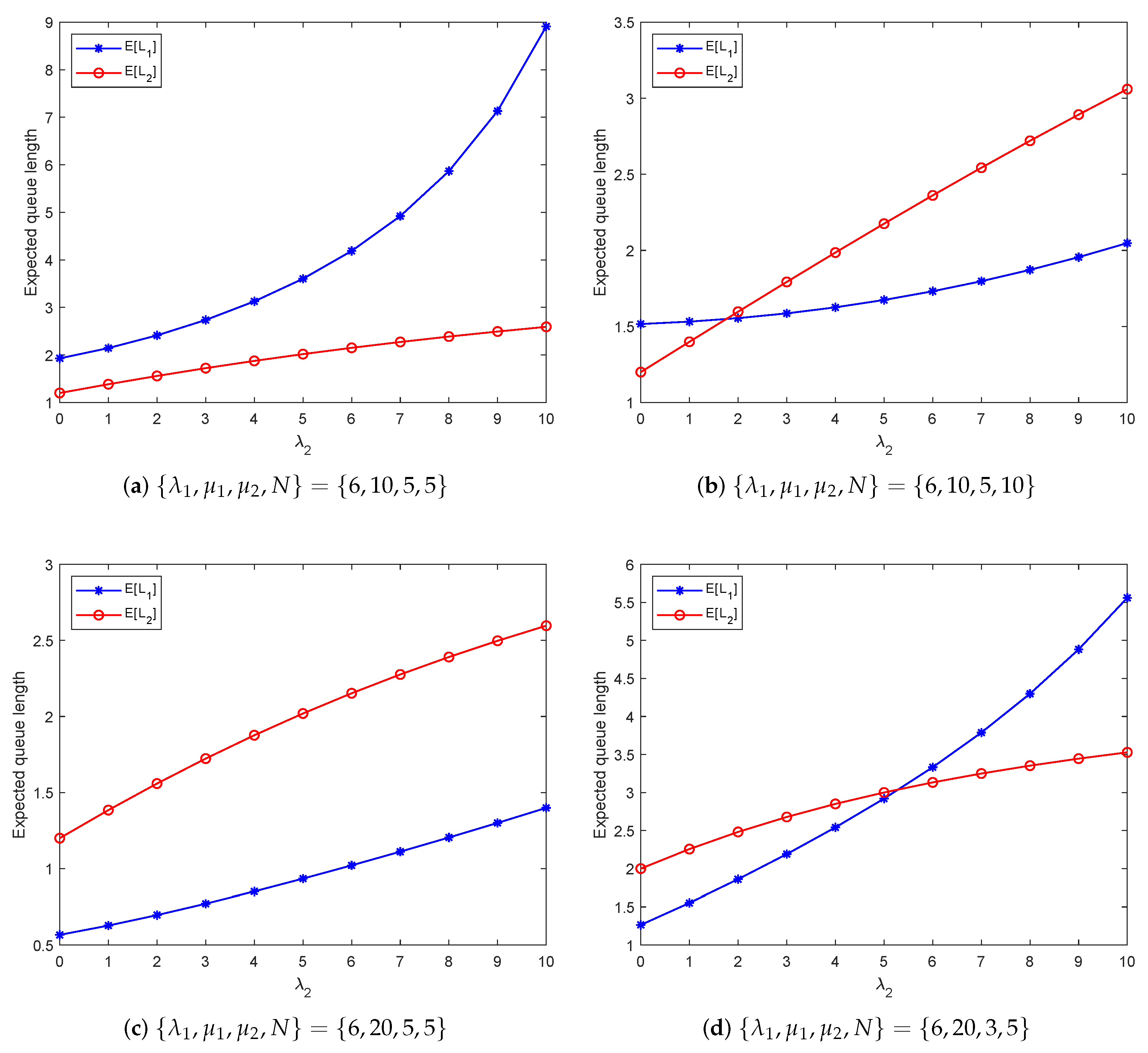
Figure 5 examines the changes in E [ L 1 ] and E [ L 2 ] as functions of the arrival rate λ 2 . With four different parameter sets, the figure demonstrates that when λ 2 increases from 0 to 10, both E [ L 1 ] and E [ L 2 ] also increase. This increase suggests that when more priority customers enter the second stage, there is a higher chance of the first stage being blocked. As a result, ordinary customers in the first stage may experience congestion.
Figure 5a,b show that when other parameters are fixed, E [ L 1 ] increases rapidly with an increase in λ 2 while E [ L 2 ] increases slowly when N = 5 . In contrast, with N = 10 , the trend reverses. This occurs because a larger N enhances the likelihood of open slots in the second stage, reducing the chance that the first stage becomes congested, thus allowing more ordinary and priority customers to advance to the second stage. Additionally, a comparison between Figure 5a,c reveals that at a constant λ 2 , a higher service rate μ 1 decreases E [ L 1 ] but elevates E [ L 2 ] . This is due to the increased flow of ordinary customers transitioning from the first to the second stage as μ 1 rises. Lastly, the outcomes in Figure 5c,d demonstrate that when all other variables are constant, the values of E [ L 1 ] and E [ L 2 ] are lower at μ 2 = 5 than at μ 2 = 3 . This is attributed to the fact that a lower μ 2 extends service times at the second stage, leading to a buildup of customers, which in turn increases the likelihood of blockages at the first stage.
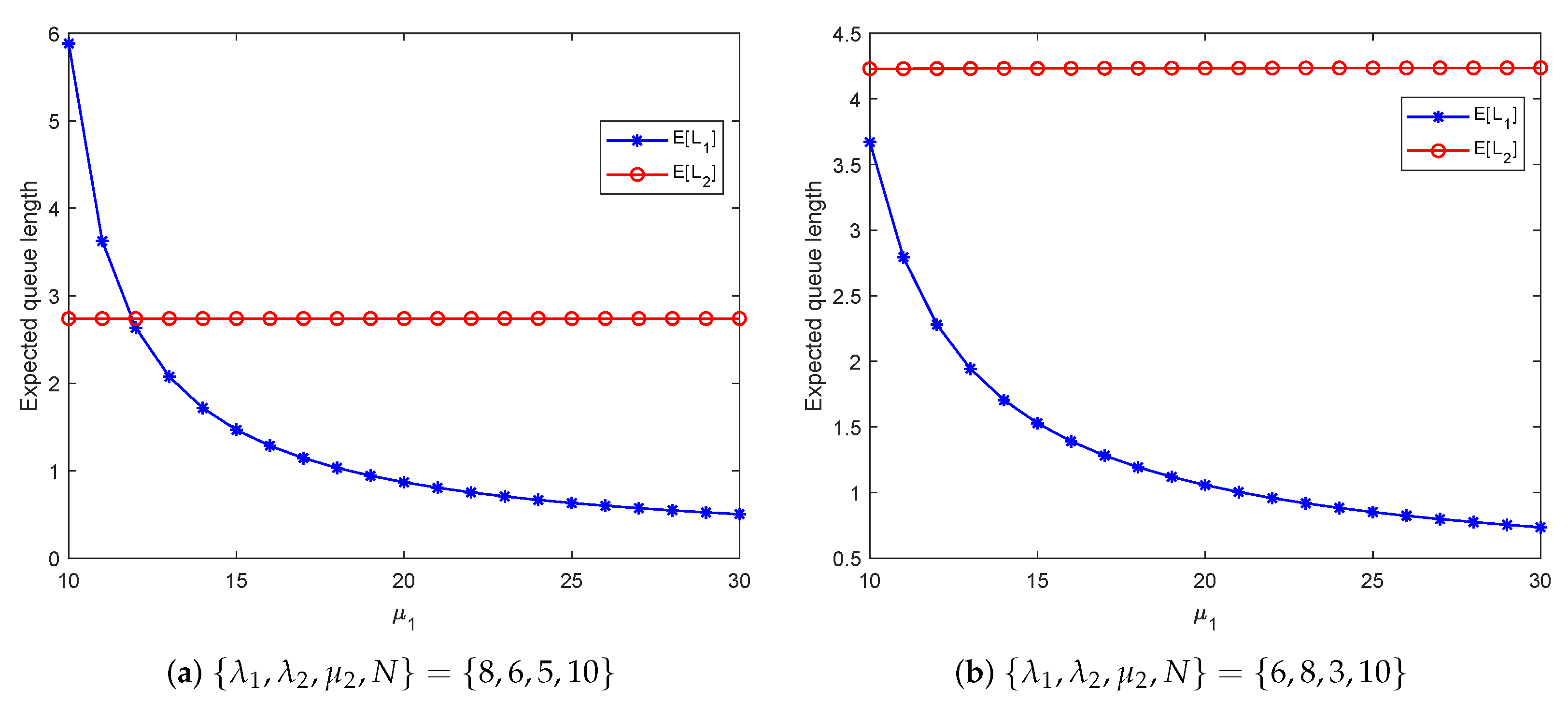
Figure 6 and Figure 7 illustrate the impact of service rates μ 1 and μ 2 on the mean queue lengths E [ L 1 ] and E [ L 2 ] . From Figure 6, we can see that as μ 1 increases, E [ L 1 ] initially decreases rapidly and then stabilizes. However, E [ L 2 ] does not show any significant change. This implies that increasing μ 1 below a certain threshold can significantly reduce the mean queue length in the first stage. However, if μ 1 is already above the threshold, further increase in the service rate will have a limited effect in reducing the mean queue length of the first stage. Figure 7 shows that E [ L 1 ] and E [ L 2 ] both gradually decrease with the increase of μ 2 and then tend to a constant value. When the service rate μ 2 is low, the second stage becomes a bottleneck for the system, resulting in queue backlog. At this point, increasing μ 2 appropriately can significantly reduce traffic intensity, decrease queue backlog, and significantly shorten the mean queue length. However, when μ 2 reaches a certain value, further increase μ 2 will not significantly change the queue length because customers in the system have already been served fast enough, and the additional service capacity has not been fully utilized.
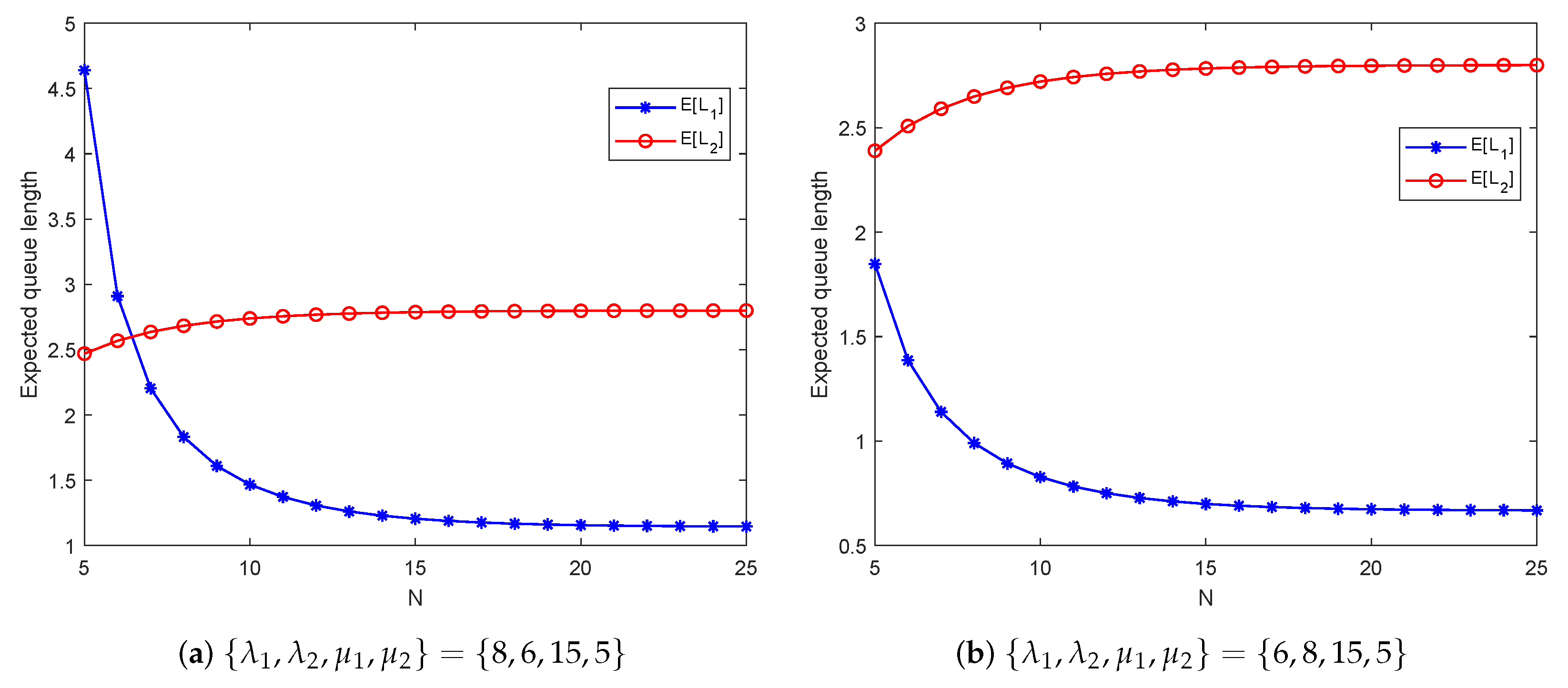
According to Figure 8, it is evident that when N < 15 , E [ L 1 ] decreases drastically as N increases. However, when N = 15 , E [ L 1 ] gradually stabilizes with the increase of N. This phenomenon arises due to the limited processing capacity of the second stage when N is small, leading to delays in customers from the first stage entering the second stage, which causes a backlog at stage one. As N increases, the second stage can accommodate more customers, facilitating a quicker transition for customers from the first stage to the second stage. Nevertheless, once N reaches a point where the second stage is no longer a bottleneck, the mean queue length in the first stage is no longer restricted by N. As for E [ L 2 ] , we can see that its change is insignificant and remains relatively stable as N increases. This indicates that the queue length in the second stage is not significantly affected by the threshold N. The reason may be the limitation of the service rate of μ 2 . Even if more customers can be accommodated, the service capabilities may not match, so the queue length will not change significantly.

6.2. Sensitivity Analysis of System Parameters on Expected Sojourn Time of an Ordinary Customer

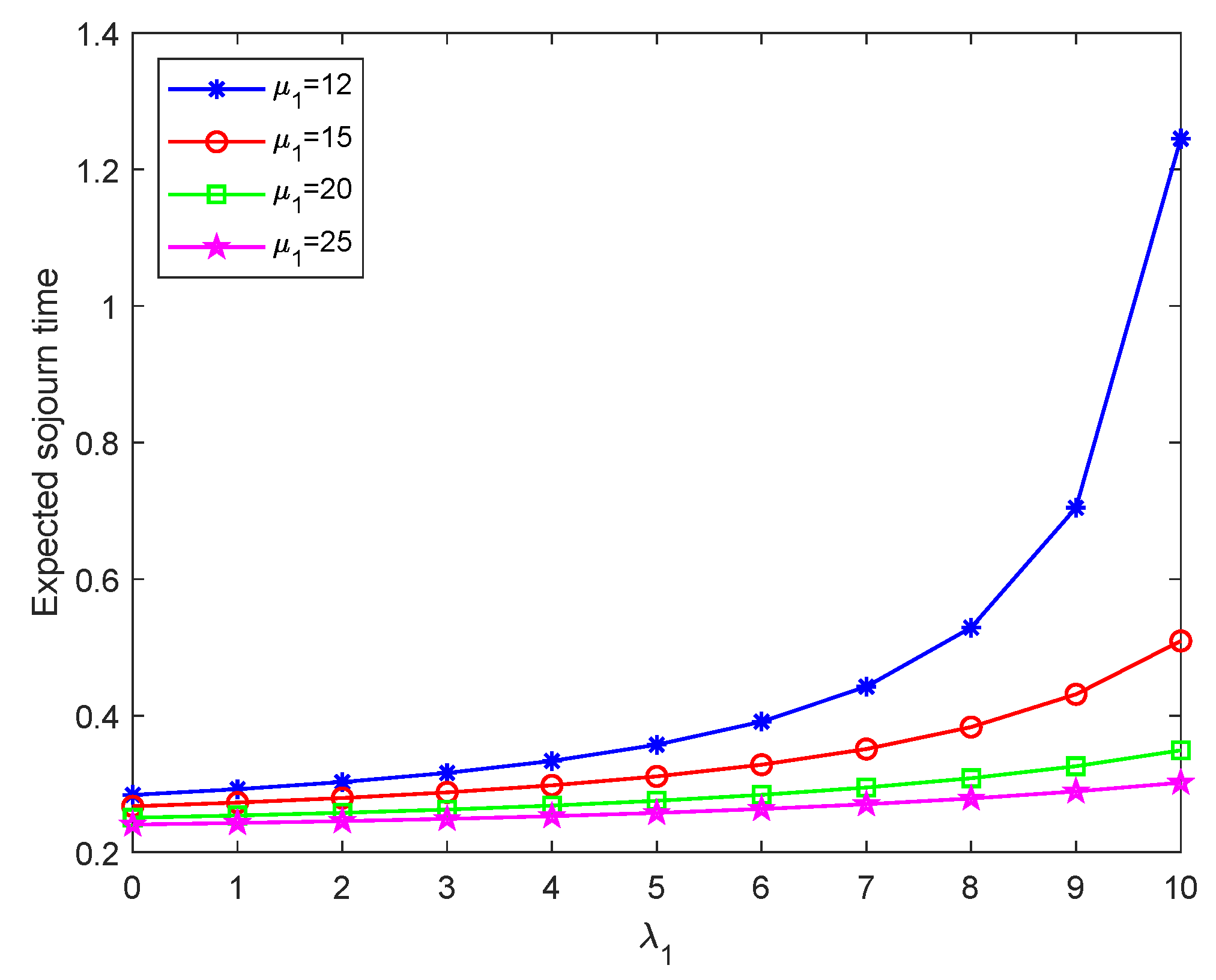
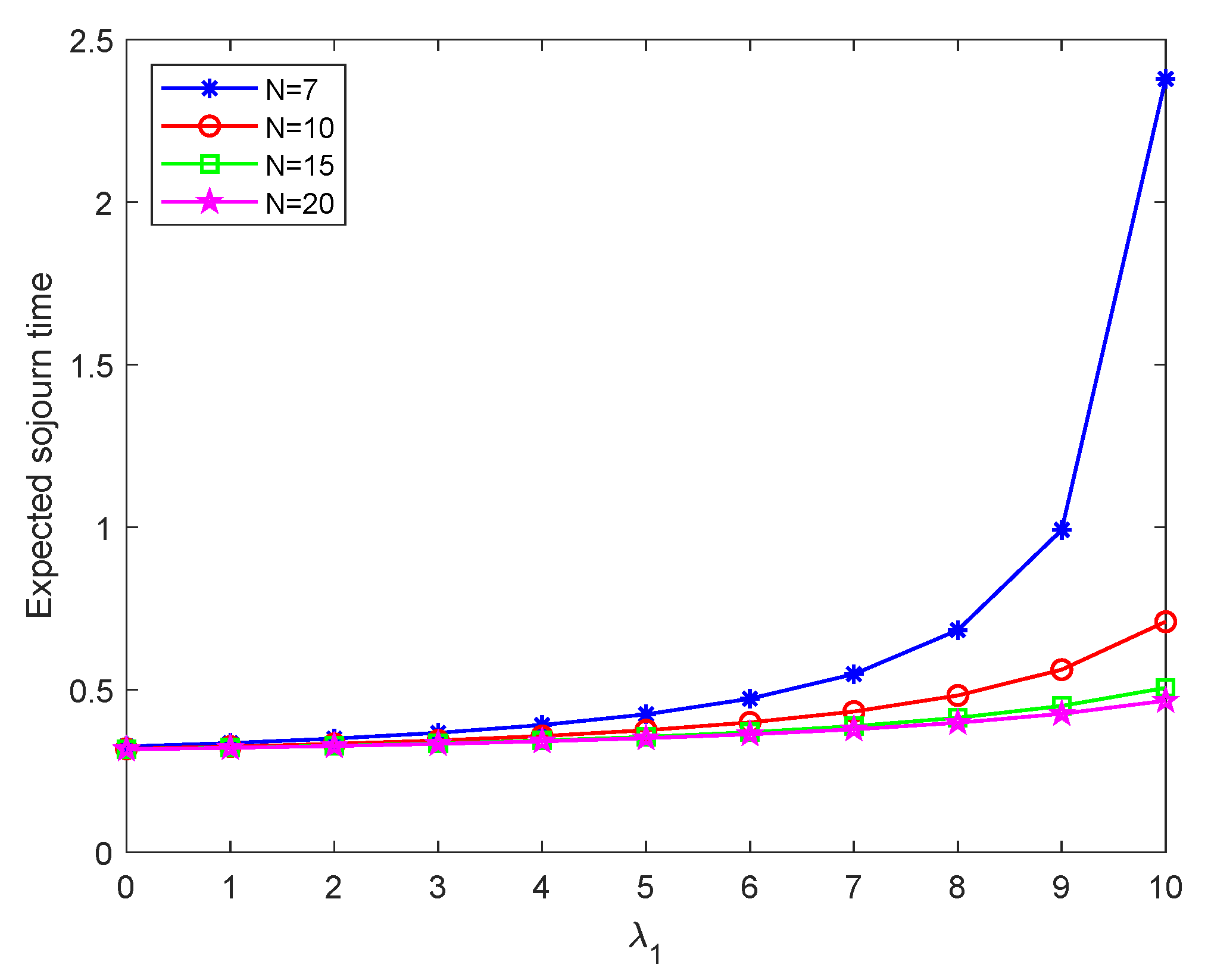
Figure 9, Figure 10, Figure 11 and Figure 12 show the expected sojourn time of ordinary customers in the system with respect to parameters λ 2 , μ 1 , μ 2 , and N as the arrival rate λ 1 increases from 0 to 10. These figures show that the expected sojourn time of ordinary customers increases with the arrival rate λ 1 increase. Because more ordinary customers reach the first stage, newly arrived ordinary customers need to wait longer to receive the first stage of service, therefore increasing their overall sojourn time in the system.
According to Figure 9, when λ 1 is small (i.e., the arrival rate in the first stage is low), there are not many people in the system, which means the system is not close to saturation. As a result, the expected sojourn time of ordinary customers is relatively short. In such a scenario, even if more priority customers enter the second stage, the system still has sufficient service capability to serve customers, so there is no significant change in sojourn time. However, when λ 1 is large, the system approaches or reaches saturation. As λ 1 increases, the second stage becomes busier and may become a bottleneck for the system. This can cause ordinary customers to be blocked in the first stage, leading to an increase in wait time. Consequently, the overall sojourn time in the system increases.
As shown in Figure 10 and Figure 11, for a given λ 1 , the expected sojourn time of ordinary customers decreases with the increase of μ 1 and μ 2 . This is because an increase in service rates leads to faster service for ordinary customers, thus reducing their sojourn time in the system. When λ 1 is small (such as λ 1 < 4 ), the difference in expected sojourn time for different μ 1 values is insignificant, and the expected sojourn time for different μ 2 values maintain low and similar values. However, when λ 1 is high (close to 10), the values of μ 1 and μ 2 significantly impact the expected sojourn time. In particular, when μ 1 = 12 or μ 2 = 3 , the expected sojourn time increases sharply, indicating that a lower service rate will significantly reduce system efficiency under a high arrival rate. For higher service rates (such as μ 1 = 25 or μ 2 = 12 ), the expected sojourn time remains low even at a higher arrival rate. That is to say, improving service efficiency is an effective strategy to reduce customer sojourn time and improve overall service quality, especially when the arrival rate is large.
Figure 12 shows that when λ 1 is small, there is not much difference in the mean sojourn time between different N values. This indicates that the capacity threshold in the second stage does not significantly impact the mean sojourn time when ordinary customers arrive less frequently. When λ 1 is large, the expected sojourn time decreases with the increase of N, especially when N is large ( N = 20 ). This means that when the system approaches saturation, a small N limits the ability of the second stage to process customers. By increasing the capacity threshold of the second stage, the pressure on the first stage can be reduced, and the overall system’s smoothness can be improved. Therefore, setting a reasonable capacity threshold for the second stage is crucial for maintaining system efficiency, especially with a large arrival rate.

6.3. Sensitivity Analysis of System Parameters on Performance Measures

Table 1, Table 2, Table 3 and Table 4 provide insights into how varying parameters λ 1 , λ 2 , μ 1 , μ 2 , and N on various system performance measures, including the probability that the first stage is empty P e 1 , the probability that the second stage is empty P e 2 , the probability that the system is empty P e , the probability of the first stage being busy P b 1 , the probability of the second stage being busy P b 2 , and the probability of the second stage running at full load P f .
As shown in Table 1 and Table 2, note that as the values of λ 1 and λ 2 increase, the probabilities P e 1 , P e 2 , and P e all decrease, which aligns with expectations. An increase in λ 1 leads to an increase in P b 1 , P b 2 , and P f . However, when λ 2 increases, only P b 2 and P f increase, while P b 1 remains constant because it is independent of the arrival rate of priority customers and is only determined by the parameters of the first stage.
Table 3 shows that as μ 1 increases, P e 1 increases while P b 1 decreases. The changes in P e 2 and P e indicate that although the service rate in the first stage improves its own performance, it has little impact on the idle state of the second stage and the entire system. Table 4 presents that when μ 2 increases, P e 2 significantly increases, while P b 2 and P f decrease. Therefore, increasing μ 1 mainly improves the congestion situation of the first stage, while increasing μ 2 not only reduces the pressure of the second stage but also reduces the congestion of the whole system and the customer’s sojourn time in the system.
In addition, from Table 3, it also can be observed that as the value of N increases, P e 1 usually increases, while P e 2 slightly decreases. This implies that the second stage of the system can accommodate more customers, which ultimately relieves the pressure on the first stage. However, P e and P b 1 do not show a consistent trend because they are more affected by μ 1 and μ 2 . The probability of full-load operation in the second stage, P f , has hardly changed, which may be because even when μ 2 is relatively small, the second stage will still quickly reach full load, even if N increases.
As shown in Table 4, with the increase of N, P e 1 increases while P e 2 decreases, which is consistent with the trend in Table 3. However, when μ 2 is large, P f significantly decreases, particularly when N is small. In summary, the impact of N on system performance indicates that increasing the second stage’s queue capacity can alleviate pressure on the first stage by allowing more customers into the second stage’s queue. Nonetheless, this effect also depends on the service rate μ 2 . With a lower μ 2 , increasing N might not substantially reduce the busyness of the second stage, as service efficiency is the limiting factor. Conversely, increasing N can effectively reduce the probabilities of busyness and full-load operation when μ 2 is sufficiently high, therefore optimizing system performance.

7. Conclusions

We analyze a two-stage tandem queuing system consisting of both ordinary and priority customers. Ordinary customers first receive service at stage one before moving on to stage two for clearing service. Priority customers bypass the first stage, directly entering the second stage for their service. We first model this system as a two-dimensional Markov chain to study the system stability condition. Subsequently, we employ the matrix-analytic method alongside spectral expansion to derive the system’s stationary distribution. We also offer analytical formulas for key characteristics, such as the expected sojourn time of ordinary customers, expected queue length, and probability of the second stage running full load. Finally, we examine the effects of various system parameters through numerical examples, providing insights that could guide the design of similar two-stage service systems.

Author Contributions

Conceptualization, J.X. and L.L.; methodology, J.X. and L.L.; software, J.X.; validation, J.X.; formal analysis, J.X.; writing—original draft preparation, J.X.; writing—review and editing, J.X. and L.L. All authors have read and agreed to the published version of the manuscript.

Funding

This research is supported by the National Natural Science Foundation of China (Grant No. 61773014).

Data Availability Statement

Data are contained within the article.

Conflicts of Interest

The authors declare no conflict of interest.

References

  1. Balsamo, S.; Persone, V.D.N.; Inverardi, P. A review on queuing network models with finite capacity queues for software architectures performance prediction. Perform. Eval. 2003, 51, 269–288. [Google Scholar] [CrossRef]
  2. Balsamo, S. Queueing networks with blocking: Analysis, solution algorithms and properties. In Network Performance Engineering: A Handbook on Convergent Multi-Service Networks and Next Generation Internet; Springer: Berlin/Heidelberg, Germany, 2011; pp. 233–257. [Google Scholar]
  3. Wang, J.; Abouee-Mehrizi, H.; Baron, O.; Berman, O. Tandem queues with impatient customers. Perform. Eval. 2019, 135, 102011. [Google Scholar] [CrossRef]
  4. Do, T.V. A closed-form solution for a tollbooth tandem queue with two heterogeneous servers and exponential service times. Eur. J. Oper. Res. 2015, 247, 672–675. [Google Scholar] [CrossRef]
  5. Jackson, J.R. Networks of waiting lines. Oper. Res. 1957, 5, 518–521. [Google Scholar] [CrossRef]
  6. VanOyen, M.P.; Teneketzis, D. Optimal stochastic scheduling of forest networks with switching penalties. Adva. Appl. Probab. 1994, 26, 474–497. [Google Scholar] [CrossRef]
  7. Katayama, T. Performance analysis and optimization of a cyclic service tandem queueing system with multi-class customers. Comput. Math. Appl. 1992, 4, 25–33. [Google Scholar] [CrossRef]
  8. Chang, K.-H.; Chen, W.-F. Admission control policies for two-stage tandem queues with no waiting spaces. Comput. Oper. Res. 2003, 30, 589–601. [Google Scholar] [CrossRef]
  9. Neuts, M.F. Two queues in series with a finite, intermediate waiting room. J. Appl. Probab. 1968, 5, 123–142. [Google Scholar] [CrossRef]
  10. Neuts, M. Matrix-Geometric Solutions in Stochastic Models; The Johns Hopkins University Press: Baltimore, MD, USA, 1981. [Google Scholar]
  11. Yang, W.-S.; Kim, T.; Park, H.; Lim, D. Analysis of a two-stage queue with a single server and N-policy. Am. J. Math. Manag. Sci. 2016, 35, 261–270. [Google Scholar] [CrossRef]
  12. Nazarov, A.; Phung-Duc, T.; Paul, S.; Morozova, M. Scaling limits of a tandem queue with two infinite orbits. Mathematics 2023, 11, 2454. [Google Scholar] [CrossRef]
  13. Dudin, S.A.; Dudina, O.S.; Dudin, A.N. Analysis of tandem queue with multi-server stages and group service at the second stage. Axioms 2024, 13, 214. [Google Scholar] [CrossRef]
  14. Choi, B.D.; Chang, Y. Single server retrial queues with priority calls. Math. Comput. Modell. 1999, 30, 27–32. [Google Scholar] [CrossRef]
  15. Gómez-Corral, A. Analysis of a single-server retrial queue with quasi-random input and non-preemptive priority. Comput. Math. Appl. 2020, 43, 767–782. [Google Scholar] [CrossRef]
  16. Walraevens, J.; Steyaert, B.; Bruneel, H. A preemptive repeat priority queue with resampling: Performance analysis. Ann. Oper. Res. 2006, 146, 189–202. [Google Scholar] [CrossRef]
  17. Artalejo, J.R.; Dudin, A.N.; Klimenok, V.I. Stationary analysis of a retrial queue with preemptive repeated attempts. Oper. Res. Lett. 2001, 28, 173–180. [Google Scholar] [CrossRef]
  18. Kim, C.; Klimenok, V.I.; Dudin, A.N. Priority tandem queueing system with retrials and reservation of channels as a model of call center. Comput. Ind. Eng. 2016, 96, 61–71. [Google Scholar] [CrossRef]
  19. Liu, B.; Zhao, Y.Q. Tail asymptotics for the M1, M2/G1, G2/1 retrial queue with non-preemptive priority. Queueing Syst. 2020, 96, 169–199. [Google Scholar] [CrossRef]
  20. Lee, S.; Dudin, S.; Dudina, O.; Kim, C.; Klimenok, V. A priority queue with many customer types, correlated arrivals and changing priorities. Mathematics 2020, 8, 1292. [Google Scholar] [CrossRef]
  21. Kim, C.; Dudin, S. Priority tandem queueing model with admission control. Comput. Ind. Eng. 2011, 61, 131–140. [Google Scholar] [CrossRef]
  22. Atencia, I. A Geo/G/1 retrial queueing system with priority services. Eur. J. Oper. Res. 2017, 256, 178–186. [Google Scholar] [CrossRef]
  23. Xie, J.; Zhu, T.; Chao, A.K.; Wang, S. Performance analysis of service systems with priority upgrades. Ann. Oper. Res. 2017, 253, 683–705. [Google Scholar] [CrossRef]
  24. Xu, J.; Liu, L.; Wu, K. Analysis of a retrial queueing system with priority service and modified multiple vacations. Comm. Stat. Theory Methods 2023, 52, 6207–6231. [Google Scholar] [CrossRef]
  25. Chamberlain, J.; Starobinski, D. Social welfare and price of anarchy in preemptive priority queues. Oper. Res. Lett. 2020, 48, 530–533. [Google Scholar] [CrossRef]
  26. Mitrani, I.; Chakka, R. Spectral expansion solution for a class of Markov models: Application and comparison with the matrix-geometric method. Perform. Eval. 1995, 23, 241–260. [Google Scholar] [CrossRef]
  27. Haverkort, B.R.; Ost, A. Steady-state analysis of infinite stochastic Petri nets: Comparing the spectral expansion and the matrix-geometric method. In Proceedings of the Seventh International Workshop on Petri Nets and Performance Models, Saint Malo, France, 3–6 June 1997; pp. 36–45. [Google Scholar]
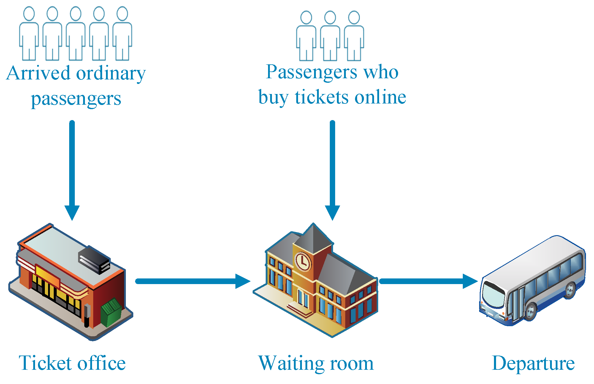
Figure 1. An example of the studied two-stage tandem queue.
Mathematics 12 01500 g001
Figure 2. Two-stage tandem queuing system with single and clearing service.
Mathematics 12 01500 g002
Figure 3. State-transition diagram of the queuing system.
Mathematics 12 01500 g003
Figure 4. Expected queue length versus the arrival rate λ 1 .
Mathematics 12 01500 g004
Figure 5. Expected queue length versus the arrival rate λ 2 .
Mathematics 12 01500 g005
Figure 6. Expected queue length versus the service rate μ 1 .
Mathematics 12 01500 g006
Figure 7. Expected queue length versus the service rate μ 2 .
Mathematics 12 01500 g007
Figure 8. Expected queue length versus the threshold queue size of the second stage N.
Mathematics 12 01500 g008
Figure 9. Expected sojourn time of ordinary customer in the system versus the arrival rate λ 2 .
Mathematics 12 01500 g009
Figure 10. Expected sojourn time of ordinary customer in the system versus the service rate μ 1 .
Mathematics 12 01500 g010
Figure 11. Expected sojourn time of ordinary customer in the system versus the service rate μ 2 .
Mathematics 12 01500 g011
Figure 12. Expected sojourn time of ordinary customer in the system versus the threshold queue size of the second stage N.
Mathematics 12 01500 g012
Table 1. Performance measures versus λ 1 with λ 2 = 6 , μ 1 = 15 , μ 2 = 5 , N = 10 .
λ 1 P e 1 P e 2 P e P b 1 P b 2 P f
10.93230.41640.38850.06670.58360.0046
20.86370.38400.33220.13330.61600.0078
30.79390.35590.28350.20000.64410.0122
40.72290.33130.24100.26670.66870.0176
50.65040.30960.20330.33330.69040.0243
60.57660.29010.16960.40000.70990.0320
70.50130.27260.13920.46670.72740.0408
80.42450.25680.11170.53330.74320.0507
90.34630.24230.08660.60000.75770.0616
Table 2. Performance measures versus λ 2 with λ 1 = 8 , μ 1 = 15 , μ 2 = 5 , N = 10 .
λ 2 P e 1 P e 2 P e P b 1 P b 2 P f
10.45630.35450.16300.53330.64550.0125
20.45170.32990.15060.53330.67010.0182
30.44610.30830.13940.53330.69170.0249
40.43970.28920.12930.53330.71080.0326
50.43240.27210.12010.53330.72790.0413
60.42450.25680.11170.53330.74320.0507
70.41590.24300.10400.53330.75700.0608
80.40690.23050.09690.53330.76950.0715
90.39730.21910.09030.53330.78090.0827
Table 3. Performance measures versus μ 1 and N with λ 1 = 8 , λ 2 = 6 , μ 2 = 7 .
N μ 1 P e 1 P e 2 P e P b 1 P b 2 P f
100.04930.31150.01640.80000.68850.1545
150.33880.31050.11290.53330.68950.1537
5200.48360.30980.16120.40000.69020.1532
250.57050.30930.19020.32000.69070.1529
300.62840.30890.20950.26670.69110.1526
100.18360.33100.06120.80000.66900.0179
150.45260.33080.15090.53330.66920.0179
10200.58710.33070.19570.40000.66930.0179
250.66780.33070.22260.32000.66930.0178
300.72160.33060.24050.26670.66940.0178
100.19790.33300.06600.80000.66700.0023
150.46490.33300.15500.53330.66700.0023
15200.59830.33300.19940.40000.66700.0023
250.67840.33300.22610.32000.66700.0023
300.73180.33300.24390.26670.66700.0023
100.19970.33330.06660.80000.66670.0003
150.46640.33330.15550.53330.66670.0003
20200.59980.33330.19990.40000.66670.0003
250.67980.33330.22660.32000.66670.0003
300.73310.33330.24440.26670.66670.0003
Table 4. Performance measures versus μ 2 and N with λ 1 = 8 , λ 2 = 6 , μ 1 = 20 .
N μ 2 P e 1 P e 2 P e P b 1 P b 2 P f
30.05810.11050.01030.40000.88950.5535
50.36980.22410.09730.40000.77590.2744
580.51370.34520.18680.40000.65480.1181
100.54950.40500.22900.40000.59500.0735
150.58320.51300.30170.40000.48700.0272
30.45210.15850.07980.40000.84150.1714
50.56070.25650.14760.40000.74350.0505
1080.59220.36200.21530.40000.63800.0111
100.59690.41600.24870.40000.58400.0046
150.59960.51710.31010.40000.48290.0007
30.55040.17040.09710.40000.82960.0589
50.59200.26180.15580.40000.73820.0104
1580.59920.36350.21790.40000.63650.0011
100.59980.41660.24990.40000.58340.0003
150.60000.51720.31030.40000.48280.0000
30.58210.17430.10270.40000.82570.0213
50.59830.26290.15740.40000.73710.0022
2080.59990.36360.21820.40000.63640.0001
100.60000.41670.25000.40000.58330.0000
150.60000.51720.31030.40000.48280.0000
Disclaimer/Publisher’s Note: The statements, opinions and data contained in all publications are solely those of the individual author(s) and contributor(s) and not of MDPI and/or the editor(s). MDPI and/or the editor(s) disclaim responsibility for any injury to people or property resulting from any ideas, methods, instructions or products referred to in the content.