On the Control Policy of a Queuing–Inventory System with Variable Inventory Replenishment Speed

Abstract

This paper considers a make-to-order production–inventory system that comprises a production facility and an inventory warehouse. Customers arrive at the facility to place an order, and the orders are processed using the first-come-first-served (FCFS) discipline. The warehouse supplies inventory items (raw materials) for the production process, and the warehouse inventory is replenished by internal production. The speed of internal production can be controlled through additional costs. If the inventory level drops to zero, the unmet demand waits in the facility until the inventory is replenished. During the stockout period, newly arriving demand is lost. The stationary joint probability of unmet demands and inventory items is derived, and a cost model is constructed. The optimal control policy for internal production is investigated to minimize the cost per unit time of the system. The experimental results show that such a production speed adjustment could reduce costs by up to 42% compared to the cases without the adjustment.

1. Introduction

The relationship between inventory management and manufacturing processes continues to be a critical factor in determining operational effectiveness within the domain of production and inventory management. This study introduces a new production facility model integrated with an inventory warehouse that is distinguished by its adaptive inventory replenishment methodology. At the core of this model lies a strategic approach to inventory management: a system designed to escalate the pace of inventory production when stock levels descend below a predetermined threshold. This mechanism stands to address the dual challenges of fluctuating demand patterns and the optimization of inventory-related costs. Operating within the framework of make-to-order production, the system manufactures finished products on demand in response to customer demands. The warehouse, a critical component of this system, supplies the necessary inventory to the production facility. These inventory items are continuously replenished via internal production.

The proposed system is based on the ‘lost sales’ assumption, where production of the finished items pauses and waits for inventory replenishment if the warehouse cannot satisfy inventory needs. During this pause, incoming customer demands are counted as lost sales. Speeding up internal production of inventory items can reduce the costs associated with these lost sales but also incur extra costs, complicating cost management. Effective cost analysis and optimization are thus crucial and complex. This paper introduces the system as a queueing-inventory model and explores the cost optimization problem. The schematic diagram of the proposed model is shown in Figure 1.

This study extends the work of [1], who investigated a make-to-order production–inventory system utilizing internal and external batch supply methods for inventory replenishment. Diverging from their methodology, this research adopts a base stock model, characterized by an (S, $S-1$) policy, initiating inventory replenishment at any indication of shortfall. The model integrates internal production of inventory items, featuring two distinct production modes: the high-cost, high-speed mode, and the low-cost, normal mode. The high-speed mode, albeit elevating production costs and necessitating frequent activation of production equipment, effectively diminishes the costs associated with lost sales. In contrast, the normal mode presents a cost-effective production alternative, reducing both inventory production costs and expenses related to equipment activation per unit time, but potentially elevating lost-sales costs due to inventory shortages.

While acknowledging the observations of Cohen and Mahafzah [2] on the complexities of parallel program characteristics and the potential limitations of assuming exponential distributions in computer and production–inventory systems, this research opts for the M/M/1 queue model and exponentially distributed inventory production time for its analytical simplicity. This choice is made with an understanding of the model’s constraints in accurately capturing more complex distribution patterns in arrival intervals and service times. Therefore, investigating models that more precisely represent general distribution patterns remains an area for future studies.

The central contribution of this research is the demonstration of substantial cost reduction through strategic adjustments in inventory production speed. The objective is to identify and implement an optimal operational strategy that balances different production modes to minimize overall costs. The proposition is that careful adjustments in production speed can result in significant cost savings, surpassing traditional methods restricted to these two modes. Numerical studies presented in Section 5 validate this, indicating potential cost reductions of up to 42%. This highlights the significant financial benefits of modulating production speed in inventory management, which is the primary focus of this research.

2. Literature Review and Motivation

In this paper, the proposed system is modeled as a type of queuing–inventory model. The queuing–inventory model is a stochastic process that combines a queuing model, and an inter-correlated inventory model. In the model, customers arrive at a server to place an order for finished goods, and the server processes the customers’ demands. The system has a finite inventory storage that contains the raw material for the production of goods. The inventory is managed according to a predetermined control policy.

Historical exploration in this domain began with the ‘assembly-like queue’ and ‘kitting queue’ studies [3,4,5,6], paving the way for subsequent analyses focused on cost-efficient management of production and manufacturing systems [7,8,9]. Application models for production systems were furthered by He and Jewkes [10] and He et al. [11].

More contemporary research has delved into the nuanced aspects of the joint probability distribution of queue length and inventory level [12,13]. Schwarz et al. [12] conducted an extensive study on the joint probability of models under the lost-sales assumption, random lead times, and various inventory control policies. Later, Schwarz and Daduna [13] studied models with the back-ordering assumption instead of lost sales. More details on the joint probability for queuing–inventory models can be found in [1,14,15,16,17,18].

Next, researchers focused on diverse customers (demand), inventory, and service characteristics. Zhao and Lian [19] studied a priority M/M/1 queuing–inventory model with two demand classes. Benny et al. [20] studied a model with two types of inventory items. They derived the stationary joint distribution by adapting the (s,S) control policy for each commodity item. A model with various service types was investigated by Mathew et al. [21], wherein the server owns two channels for service: one channel for a single service and the other channel for batch service. Models with customer retrials were studied by Krishnamoorthy and Shajin [22] and Krishnamoorthy et al. [23]. For more details on systems with generalized arrival processes, readers are referred to Chakravarthy et al. [24] and the references therein.

Recent developments in queuing–inventory system research have emphasized the integration of customer priority and the management of unpredictable disruptions, leading to more nuanced and realistic models. Liu et al. [25] and Jeganathan et al. [26] have been instrumental in incorporating customer priorities into QIS. Liu et al. developed a model for systems like airlines and railways, focusing on level-dependent retrial rates influenced by customer perceptions of wait times, while Jeganathan et al. introduced a threshold-based inventory level affecting customer service priority. These studies collectively highlight the importance of customer priority in enhancing system efficiency and customer satisfaction.

Simultaneously, Melikov et al. [27] and Ozkar et al. [28] have advanced queuing–inventory system modeling by considering negative customers and warehouse catastrophes. Melikov et al.’s single-server QIS model, using Markovian arrival processes and Phase-Type distribution, diverges from traditional approaches by combining varied replenishment policies. Ozkar et al. further extended this framework, examining two QISs with both (s,S) and (s,Q) policies, offering deeper insights into system performance under complex scenarios. Together, these studies represent significant strides in QIS research, underscoring the need for models that account for both internal customer dynamics and external operational challenges.

Recent advancements in queuing–inventory system research have addressed key issues like customer priority integration and responses to unpredictable disruptions. However, there is a significant gap in exploring the concept of variable inventory production speed within these models. Although previous research has extensively analyzed aspects such as customer retrials, priority levels, the impact of negative customers, and warehouse catastrophes, it has not sufficiently delved into the relationship between inventory production speed and inventory levels, which is vital for enhancing service efficiency and managing costs.

This lack of exploration in dynamically adjusting inventory production speed according to the levels represents a critical area for further research. The primary focus of this study is to introduce a new model that facilitates such optimization. This proposed model is designed to better understand and manage the interplay between inventory replenishment speed and its associated costs, thereby offering a framework for more efficient inventory management strategies.

The remainder of this paper is organized as follows: Section 3 describes the proposed model in detail, introducing a novel modified model crucial for the ensuing analysis. Basic model assumptions are introduced followed by a summary of notation. Section 4 is devoted to deriving the stationary joint probability distribution and delineating the system performance measures in explicit form. Section 5 is reserved for the construction and evaluation of the cost model supplemented with illustrative numerical examples. The paper culminates in Section 6 with concluding remarks, offering insights into potential generalizations and the broader applicability of the model.

3. The System and the Model

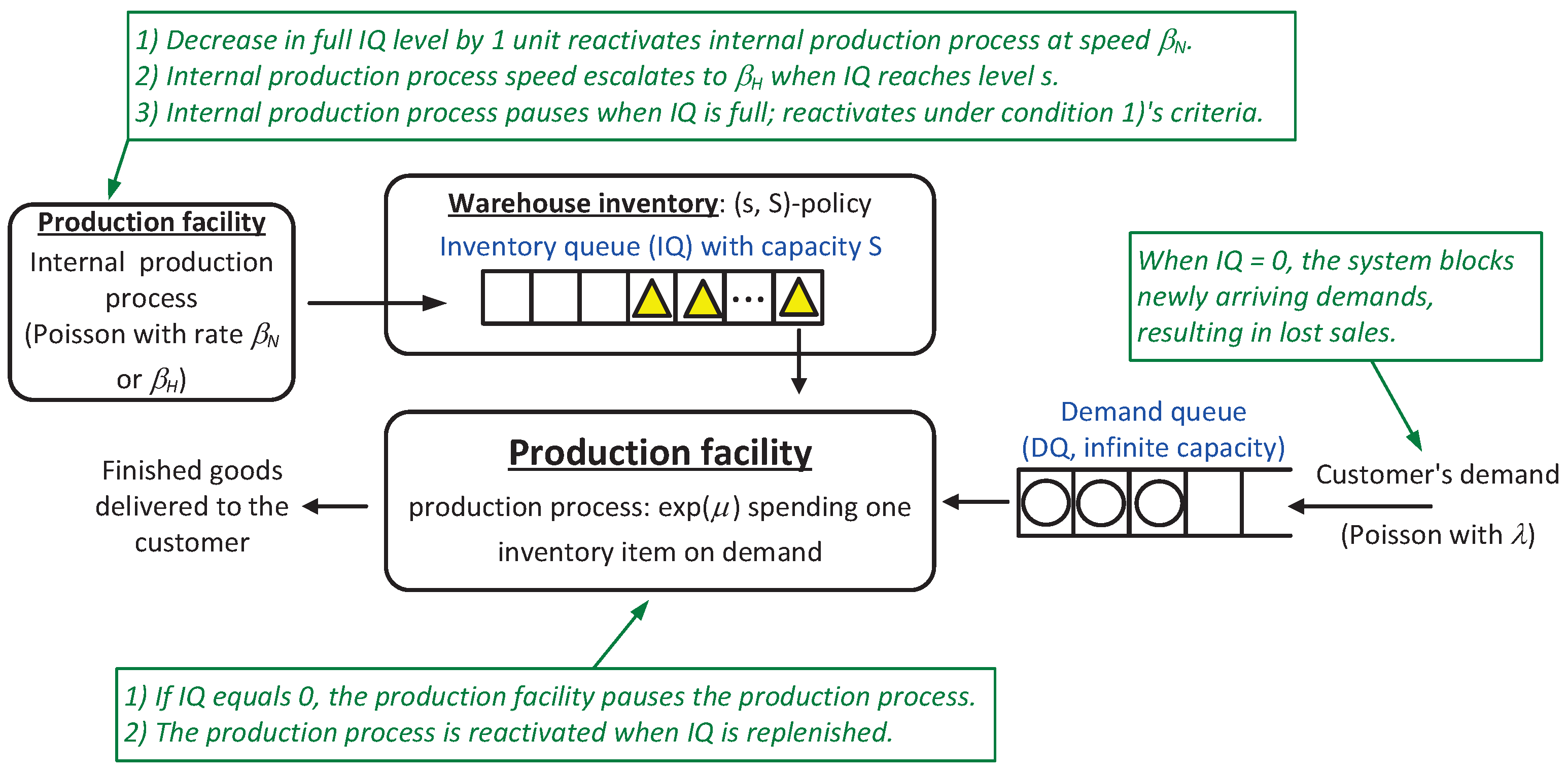
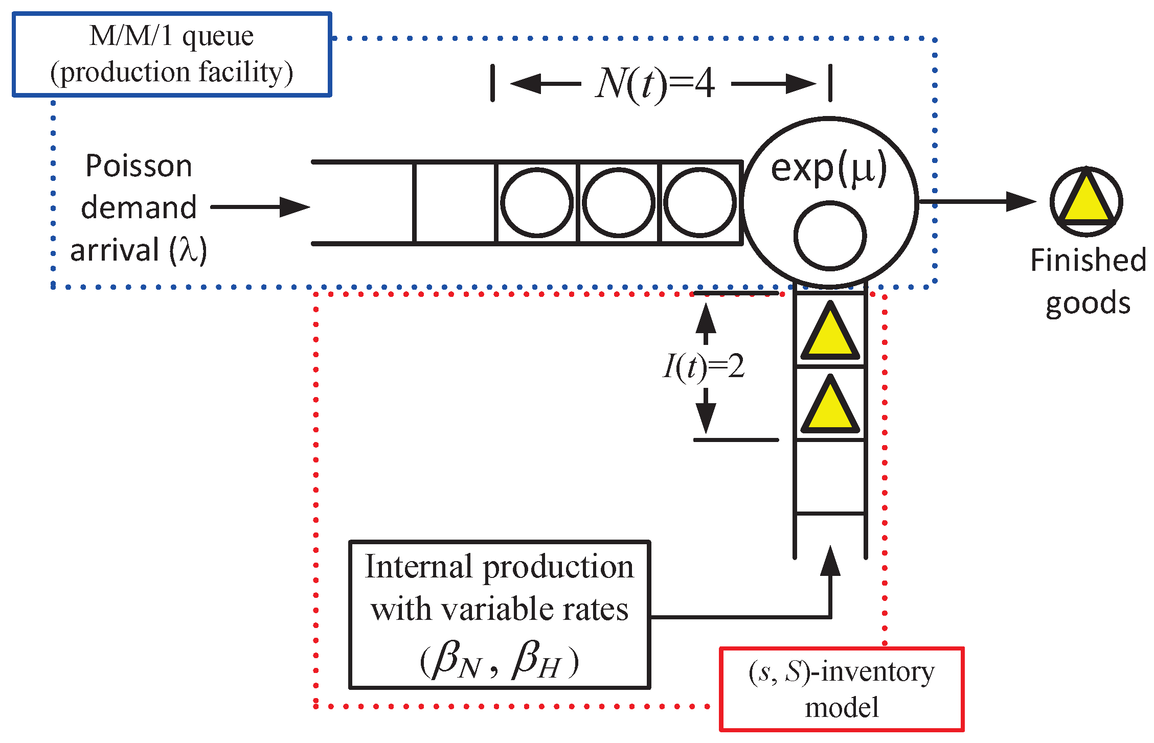
This section describes the proposed model in detail and introduces a modified model for the analysis.

3.1. The Model

The proposed system, as illustrated in Figure 1, is modeled as a production–inventory system encompassing both a production facility and an attached inventory warehouse (refer to Figure 2). The warehouse’s inventory storage, with a capacity of S, stores raw materials. The operational framework of the proposed model is based on a set of fundamental assumptions, which are summarized as follows:

• Customers arrive at the system according to a Poisson process with a rate of $\lambda$. Upon arrival, they place orders (demands) for finished products.
• Orders are processed by the server on a first-come-first-served basis; the server thus produces the finished goods according to the sequence of orders.
• Upon completion of each of the finished goods, the server consumes an item from the warehouse inventory.
• The system adheres to a ’lost sales’ policy; customers who find the inventory empty upon their arrival will immediately leave the system without being served, resulting in a lost-sales cost.
• The warehouse inventory is continuously replenished through internal production, which operates in two distinct modes: a normal mode and a high-speed mode.
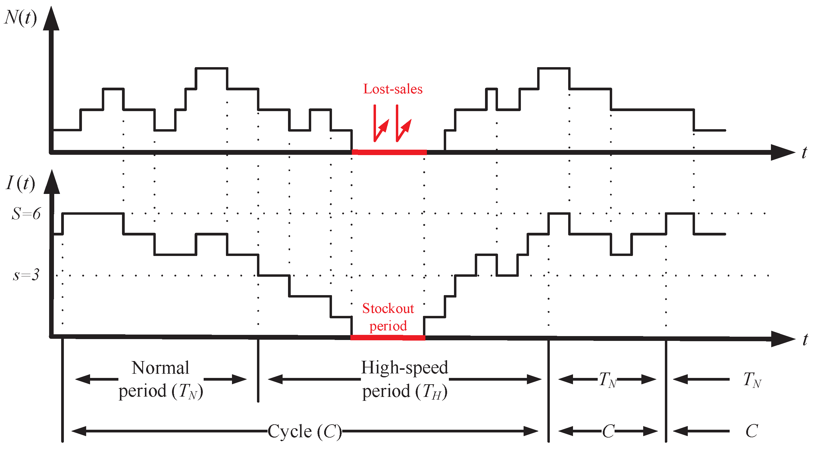
• Once the inventory level drops to s, the high-speed mode is activated, and then the mode is switched back to normal as soon as the warehouse is restocked to its full capacity, which is denoted as S.
• The production times for inventory items and the manufacturing times for finished goods are governed by exponential distributions.

Remark 1.

Assumption 6 allows for the detailed adjustment of inventory replenishment speed in the proposed model, differing from traditional research that typically adopts a single-speed replenishment policy. This assumption forms the basis of the model and aims to demonstrate the possibility of operational cost savings through such speed adjustments.

Remark 2.

Assumption 7, which adopts exponential distributions for the production times, was chosen for its analytical simplicity as outlined in Section 1. This simplification enables a concentrated examination of the effects of varying inventory production speeds. However, it is important to note that this may not fully represent the more complex distribution patterns that can occur in real-world systems.

The notations used for the proposed model are summarized as follows:

-

$\lambda$: arrival rate of customers;

-

$1/\mu$: expected production time of a finished product;

-

$1/{\beta }_N$: expected production time of an inventory item in normal mode;

-

$1/{\beta }_H$:expected production time of an inventory item in high-speed mode;

-

s: the threshold level of inventory to activate the high-speed mode;

-

S: the capacity of the ready-to-use inventory storage;

-

$N\left(t\right)$: the number of unmet orders in the system at time t;

-

$I\left(t\right)$: the amount of ready-to-use inventory in the system at time t.

Figure 3 depicts a typical sample path of the model for $S=6$ and $s=3$. At any given time t, $N\left(t\right)$ indicates the number of unmet demands, and $I\left(t\right)$ shows the inventory level. The production system of the finished goods is modeled as an M/M/1 queue, where the production times are independent, identically distributed exponential random variables with mean $\frac{1}{\mu }$. Each unit of production consumes one inventory item. When the warehouse runs out of stock, the server pauses and awaits inventory replenishment. Under the lost sales assumption, any new demand that arrives during this out-of-stock period is considered lost, incurring a cost for lost sales.

The warehouse inventory is replenished by internal production under two production modes: normal and high-speed. The normal mode is triggered when the inventory level reaches S. In this mode, the replenishment follows a Poisson process with rate ${\beta }_N$ where ${\beta }_N<\lambda$. The high-speed mode commences as the inventory level falls to s, with the replenishment rate increasing to ${\beta }_H$, satisfying $\lambda <{\beta }_H$. This high-speed mode continues until the inventory is fully restocked.

The length of time from level S to the threshold level s, as determined by the first passage time, is defined as a ‘normal period’ and is denoted by $T_N$. The ‘high-speed period’, denoted by $T_H$, is defined by the length of the first passage time needed to return to level S from the threshold level s. Additionally, a ‘cycle’, represented by C, refers to the length of the first returning time required to reach level S once again, thereby completing a full cycle of this process. Thus, a cycle consists of two distinct phases: a normal period followed potentially by a high-speed period. Note that the unmet demand process $\left\{N\right(t):t\ge 0\}$ strictly depends on the warehouse inventory process $\left\{I\right(t):t\ge 0\}$. However, the inventory level process behaves as a regenerative process in which the normal period starting points are the regeneration points. This concept of the regenerative process plays an important role in analyzing the proposed model.

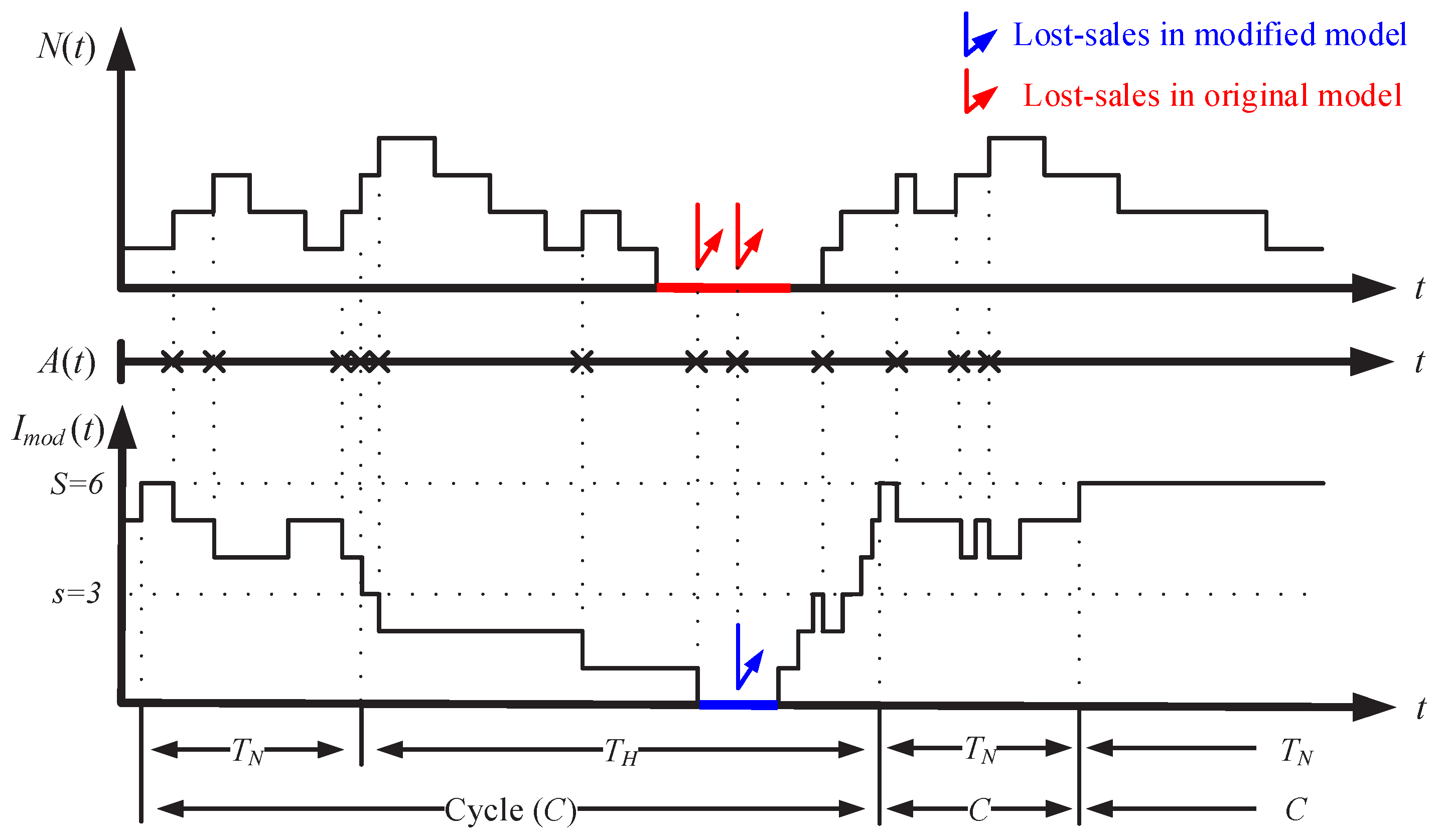
3.2. The Modified Model

This section presents a modified model, designed to facilitate both effective and efficient analysis of the proposed model.

Definition 1

(Modified Model, Krishnamoorthy and Viswanath [17]). The modified model represents a specific variant of the proposed model, characterized by setting the production times of the facility to zero.

Figure 4 presents a comparison between the modified model’s sample path and the unmet demand process of the proposed model, both plotted on the same time scale. The upper section of the figure displays the unmet demand process, $\left\{N\right(t):t\ge 0\}$, from the original model and the arrival process, $\left\{A\right(t):t\ge 0\}$. The figure also depicts the inventory level process of the modified model as $\{I_{mod}:t\ge 0\}$, demonstrating an immediate decrease in inventory upon demand arrival, which is a consequence of assuming zero production time. Therefore, the modified model can be viewed as a stochastic inventory system, where demands arrive according to a Poisson process with rate $\lambda$, and inventory replenishment is conducted as outlined in Section 3.1.

For analysis of the modified model, an indicator function $\xi \left(t\right)$ is defined as

$$\xi \left(t\right)=\left\{\begin{array}{cc}1,\hfill & \mathrm{if}\mathrm{the}\mathrm{system}\mathrm{is}\mathrm{in}\mathrm{normal}\mathrm{mode}\mathrm{at}\mathrm{time}t,\hfill \\ 2,\hfill & \mathrm{if}\mathrm{the}\mathrm{system}\mathrm{is}\mathrm{in}\mathrm{high}\text{-}\mathrm{speed}\mathrm{mode}\mathrm{at}\mathrm{time}t.\hfill \end{array}\right.$$

Every normal period starts with S warehouse inventory items. Moreover, the inter-arrival times of the demands and internal production times follow exponential distributions. Therefore, the process $\{(I_{mod}\left(t\right),\xi \left(t\right)):t\ge 0\}$ becomes a Markov process. Next, the following probabilities are defined

$${\chi }_N(k,t)=Pr[I\left(t\right)=k,\xi \left(t\right)=1],$$

$${\chi }_H(k,t)=Pr[I\left(t\right)=k,\xi \left(t\right)=2],$$

$${\chi }_N\left(k\right)=\underset{t\to \infty }{lim}{\chi }_N(k,t),{\chi }_H\left(k\right)=\underset{t\to \infty }{lim}{\chi }_H(k,t),$$

to obtain the following steady-state equations:

$$\begin{array}{c}\hfill \lambda {\chi }_N\left(S\right)={\beta }_N{\chi }_N(S-1)+{\beta }_H{\chi }_H(S-1)\end{array}$$

(1)

$$\begin{array}{c}\hfill ({\beta }_N+\lambda ){\chi }_N\left(k\right)={\beta }_N{\chi }_N(k-1)+\lambda {\chi }_N(k+1),s+2\le k\le S-1,\end{array}$$

(2)

$$\begin{array}{c}\hfill (\lambda +{\beta }_N){\chi }_N(s+1)=\lambda {\chi }_N(s+2)\end{array}$$

(3)

$$\begin{array}{cc}\hfill (\lambda +{\beta }_H){\chi }_H\left(k\right)=& {\beta }_H{\chi }_H(k-1)+\lambda {\chi }_H(k+1),k=1,\dots ,s-1,s+1,\dots ,S-1,\hfill \end{array}$$

(4)

$$\begin{array}{cc}\hfill & (\lambda +{\beta }_H){\chi }_H\left(s\right)={\beta }_H{\chi }_H(s-1)+\lambda {\chi }_N(s+1)+\lambda {\chi }_H(s+1),\hfill \end{array}$$

(5)

$$\begin{array}{c}\hfill {\beta }_H{\chi }_H\left(0\right)=\lambda {\chi }_H\left(1\right)\end{array}$$

(6)

4. Analysis

This section derives the stationary joint probability of the proposed model in closed form and then obtains the mean performance measures explicitly.

4.1. The Joint Probability Distribution

The following probabilities are defined for constructing the steady-state equations of the original process $\left\{\right(N\left(t\right),I\left(t\right),\xi \left(t\right)):t\ge 0\}$:

$$X_N(n,k,t)=Pr[N\left(t\right)=n,I\left(t\right)=k,\xi \left(t\right)=0],$$

$$X_H(n,k,t)=Pr[N\left(t\right)=n,I\left(t\right)=k,\xi \left(t\right)=1],$$

$$X_N(n,k)=\underset{t\to \infty }{lim}{X}_N(n,k,t),X_H(n,k)=\underset{t\to \infty }{lim}{X}_H(n,k,t).$$

Then, the following system equations are given:

$$\begin{array}{c}\hfill 0=-\lambda X_N(0,S)+{\beta }_N{X}_N(0,S-1)+{\beta }_H{X}_H(0,S-1),\end{array}$$

(7)

$$\begin{array}{cc}\hfill 0=& -(\lambda +\mu )X_N(n,S)+\lambda X_N(n-1,S)+{\beta }_N{X}_N(n,S-1)+{\beta }_H{X}_H(n,S-1),n\ge 1,\hfill \end{array}$$

(8)

$$\begin{array}{cc}\hfill 0=& -(\lambda +{\beta }_N)X_N(0,k)+\mu X_N(1,k+1)+{\beta }_N{X}_N(0,k-1),s+2\le k\le S-1,\hfill \end{array}$$

(9)

$$\begin{array}{cc}\hfill 0=& -(\lambda +\mu +{\beta }_N)X_N(n,k)+\lambda X_N(n-1,k)+\mu X_N(n+1,k+1)\hfill \\ \hfill & +{\beta }_N{X}_N(n,k-1),n\ge 1,s+2\le k\le S-1,\hfill \end{array}$$

(10)

$$\begin{array}{c}\hfill 0=-(\lambda +{\beta }_N)X_N(0,s+1)+\mu X_N(1,s+2),\end{array}$$

(11)

$$\begin{array}{cc}\hfill 0=& -(\lambda +\mu +{\beta }_N)X_N(n,s+1)+\lambda X_N(n-1,s+1)+\mu X_N(n+1,s+2),n\ge 1,\hfill \end{array}$$

(12)

$$\begin{array}{cc}\hfill 0=-(\lambda +{\beta }_H)X_H(0,k)& +\mu X_H(1,k+1)+{\beta }_H{X}_H(0,k-1),\hfill \\ \hfill & k=1,\dots ,s-1,s+1,s+2,\dots ,S-1,\hfill \end{array}$$

(13)

$$\begin{array}{cc}\hfill 0=-(\lambda +\mu +{\beta }_H)X_H(n,k)+& \lambda X_H(n-1,k)+\mu X_H(n+1,k+1)+{\beta }_H{X}_H(n,k-1),\hfill \\ \hfill & n\ge 1,k=1,\dots ,s-1,s+1,s+2,\dots ,S-1,\hfill \end{array}$$

(14)

$$\begin{array}{cc}\hfill 0=& -(\lambda +{\beta }_H)X_H(0,s)+\mu X_N(1,s+1)+\mu X_H(1,s+1)+{\beta }_H{X}_H(0,s-1),\hfill \end{array}$$

(15)

$$\begin{array}{cc}\hfill 0=& -(\lambda +\mu +{\beta }_H)X_H(n,s)+\lambda X_H(n-1,s)\hfill \\ \hfill & +\mu X_N(n+1,s+1)+\mu X_H(n+1,s+1)+{\beta }_H{X}_H(n,s-1),n\ge 1,\hfill \end{array}$$

(16)

$$\begin{array}{c}\hfill 0=-{\beta }_H{X}_H(0,0)+\mu X_H(1,1),\end{array}$$

(17)

$$\begin{array}{c}\hfill 0=-{\beta }_H{X}_H(n,0)+\mu X_H(n+1,1),n\ge 1.\end{array}$$

(18)

Then, following theorem is given.

Theorem 1.

Let $P\left(n\right)=\left(1-\frac{\lambda }{\mu }\right){\left(\frac{\lambda }{\mu }\right)}^n,n\ge 0$ be the queue length probability of the classical M/M/1 queue. Then, the stationary joint probability distribution of the proposed model is given as

$$\begin{array}{cc}\hfill X_N(n,k)& =P\left(n\right)·{\chi }_N\left(k\right),n\ge 0,s+1\le k\le S,\hfill \end{array}$$

(19)

$$\begin{array}{cc}\hfill X_H(n,k)& =P\left(n\right)·{\chi }_H\left(k\right),n\ge 0,0\le k\le S-1.\hfill \end{array}$$

(20)

Proof. 

The proof is given in Appendix A.    □

Remark 3.

Theorem 1 suggests that the joint probability distribution in the proposed model can be divided into two distinct components: one representing the unmet demand process and the other the warehouse inventory process. The latter is congruent with the stationary inventory level distribution in the modified model.

Remark 4.

Furthermore, the theorem states that both the conditional and marginal stationary queue length distributions of the unmet demands can be found to be equivalent to those in the standard M/M/1 queue, which are characterized by the formula $\left(1-\frac{\lambda }{\mu }\right){\left(\frac{\lambda }{\mu }\right)}^n,n\ge 0$.

Consequently, Equations (19) and (20) can be completely determined only by obtaining stationary inventory level distribution of the modified process.

4.2. Analysis of Modified Model

This section derives the stationary probabilities ${\chi }_N\left(k\right)$ and ${\chi }_H\left(k\right)$ of the modified model to complete Theorem 1.

In the modified model, every normal period starts at inventory level S, and the inter-arrival times of the demand are i.i.d exponential random variables. Therefore, the modified process $\{I_{mod}\left(t\right):t\ge 0\}$ becomes a regenerative process in which the normal period starting points play the role of regeneration points. Consequently, classical renewal theory can be applied to analyze the modified process. A normal period may end without reaching the level s, indicating that the regeneration cycle of the modified process comprises a normal period followed by a potentially ensuing high-speed period (see Figure 4).

4.2.1. Analysis of the High-Speed Period

This section derives the stationary probability ${\chi }_H\left(k\right)$ of the warehouse inventory level at an arbitrary time during a high-speed period. To achieve this, the dual inventory level process of the modified model is defined as $\{I_{mod}^{dual}\left(t\right):t\ge 0\}=\{S-I_{mod}\left(t\right):t\ge 0\}$. Then, the stationary probability ${\chi }_H\left(k\right)$ is given in the following theorem.

Theorem 2.

${\chi }_H\left(k\right)$ is given as

$$\begin{array}{c}\hfill {\chi }_H\left(k\right)=\left\{\begin{array}{cc}{\displaystyle \frac{{\left(\frac{\lambda }{{\beta }_H}\right)}^{s-k}-{\left(\frac{\lambda }{{\beta }_H}\right)}^{S-k}}{K(s,S)({\beta }_H-\lambda )}},\hfill & 0\le k\le s,\hfill \\ {\displaystyle \frac{1-{\left(\frac{\lambda }{{\beta }_H}\right)}^{S-k}}{K(s,S)({\beta }_H-\lambda )}},\hfill & s+1\le k\le S-1,\hfill \end{array}\right.\end{array}$$

(21)

where $K(s,S)$ is a normalization constant.

Proof. 

Let $T_H\left(k\right)$ and $T_H^{dual}\left(k\right)$ be the total sojourn times at warehouse inventory level k during a high-speed period in a modified process and a dual process, respectively. Then, by noting $\mathbb{E}\left[T_H\left(k\right)\right]=\mathbb{E}\left[T_H^{dual}(S-k)\right]$, ${\chi }_H\left(k\right)$ can be obtained from

$$\begin{array}{cc}\hfill {\chi }_H\left(k\right)& ={\chi }_H^{dual}(S-k)=\frac{\mathbb{E}\left[T_H^{dual}(S-k)\right]}{K(s,S)},\hfill \end{array}$$

(22)

where $\frac{1}{K(s,S)}$ is multiplied as a normalization constant.

Note that every high-speed period starts with s initial inventory items and ends as soon as the level reaches S. The demands arrive according to the Poisson process with a rate $\lambda$, and the internal production replenishes the warehouse inventory at a rate ${\beta }_H$ according to the Poisson process. This implies that the high-speed period in the dual process is stochastically identical to the busy period of the classical M/M/1/S queue starting with $(S-s)$ initial customers, in which the arrival and service rates are $\lambda$ and ${\beta }_H$, respectively. Consequently, a busy period analysis of the classical M/M/1/S queue can be applied to obtain $\mathbb{E}\left[T_H^{dual}\left(k\right)\right]$.

For the classical M/M/1/S queue with arrival rate $\lambda$ and service rate ${\beta }_H$, let $\tilde{N}\left(t\right)$ be the number of customers in the system to define the following probability:

$$\begin{array}{c}\hfill p_{\left(i\right)}(k,t|\lambda ,{\beta }_H)=Pr[\tilde{N}\left(t\right)=k,0<\tilde{N}\left(u\right)\le Sfor0\le u\le t|N\left(0\right)=i],1\le k\le S.\end{array}$$

(23)

Here, $p_{\left(i\right)}(k,t|\lambda ,{\beta }_H)$ represents the probability that a busy period of an M/M/1/S queue starting with i initial customers visits the state wherein the number of customers is k at time t. Defining ${\tilde{p}}_{\left(i\right)}\left(k\right|\lambda ,{\beta }_H)={\int }_0^{\infty }{p}_{\left(i\right)}(k,t|\lambda ,{\beta }_H)dt$, $\mathbb{E}\left[T_H^{dual}\left(k\right)\right]$ can be obtained using the following equation:

$$\mathbb{E}\left[T_H^{dual}\left(k\right)\right]={\tilde{p}}_{(S-s)}\left(k\right|\lambda ,{\beta }_H).$$

Now, a generating function ${\tilde{P}}_{\left(i\right)}\left(z\right|\lambda ,{\beta }_H)={\sum }_{k=1}^S{z}^k{\tilde{p}}_{\left(i\right)}\left(k\right|\lambda ,{\beta }_H)$ is defined, summing over all states. Then, the results in Takagi and Tarabia [29] give

$$\begin{array}{cc}\hfill {\tilde{P}}_{(S-s)}\left(z\right|\lambda ,{\beta }_H)& =\frac{z\left[z^{S-s}-1+\frac{\lambda (z-1)z^S\left[{\left(\frac{\lambda }{{\beta }_H}\right)}^s-{\left(\frac{\lambda }{{\beta }_H}\right)}^S\right]}{{\beta }_H-\lambda }\right]}{(1-z)({\beta }_H-z\lambda )},\hfill \\ \hfill & =\frac{1}{{\beta }_H-\lambda }\left[\sum _{k=1}^{S-s}{z}^k-\sum _{k=1}^S{\left(\frac{\lambda }{{\beta }_H}z\right)}^k+z^{S-s}\sum _{k=1}^s{\left(\frac{\lambda }{{\beta }_H}z\right)}^k\right].\hfill \end{array}$$

(24)

Finally, the inversion yields

$$\begin{array}{c}\hfill \mathbb{E}\left[T_H^{dual}\left(k\right)\right]=\left\{\begin{array}{cc}{\displaystyle \frac{{\left(\frac{\lambda }{{\beta }_H}\right)}^{k-(S-s)}-{\left(\frac{\lambda }{{\beta }_H}\right)}^k}{{\beta }_H-\lambda }},\hfill & S-s\le k\le S,\hfill \\ {\displaystyle \frac{1-{\left(\frac{\lambda }{{\beta }_H}\right)}^k}{{\beta }_H-\lambda }},\hfill & 1\le k\le S-s-1,\hfill \end{array}\right.\end{array}$$

(25)

and finishes the proof by noting that $\mathbb{E}\left[T_H\left(k\right)\right]=\mathbb{E}\left[T_H^{dual}(S-k)\right]$.    □

Remark 5.

Applying some algebra reveals that the stationary probability ${\chi }_H\left(k\right)$ is directly proportional to the stationary inventory level probability production period in the classical (s, S) production–inventory model (Krishnamoorthy and Viswanath [17]). Consequently, this indicates that the inventory process during high-speed periods is stochastically identical to the inventory level process during production periods in the existing study.

4.2.2. Analysis of the Normal-Speed Period

This section derives the stationary probability ${\chi }_N\left(k\right)$ of the warehouse inventory level at an arbitrary time in a normal period.

Theorem 3.

${\chi }_N\left(k\right)$ is given as

$$\begin{array}{c}\hfill {\chi }_N\left(k\right)=\frac{1}{K(s,S)}\frac{{\left(\frac{{\beta }_N}{\lambda }\right)}^{k-s}-1}{{\beta }_N-\lambda },s+1\le k\le S.\end{array}$$

(26)

Proof. 

In steady state, the expected number of departures from the normal period per unit time equals the expected number of entries into the period, resulting in the equation:

$$\begin{array}{c}\hfill \lambda {\chi }_N(s+1)={\beta }_H{\chi }_H(S-1).\end{array}$$

(27)

Applying Equation (21) in the above equation yields

$$\begin{array}{c}\hfill {\chi }_N(s+1)=\frac{1/\lambda }{K(s,S)}.\end{array}$$

(28)

Applying Equation (27) to Equation (1) gives

$$\begin{array}{c}\hfill {\chi }_N\left(S\right)=\frac{{\beta }_N}{\lambda }{\chi }_N(S-1)+{\chi }_N(s+1).\end{array}$$

(29)

In addition, using Equations (2) and (29) yields

$$\begin{array}{c}\hfill {\chi }_N\left(k\right)=\frac{{\beta }_N}{\lambda }{\chi }_N(k-1)+{\chi }_N(s+1),s+2\le k\le S-1.\end{array}$$

(30)

Then, Equations (29) and (30) can be rewritten as the following reclusive form:

$$\begin{array}{c}\hfill {\chi }_N\left(k\right)+\frac{\lambda {\chi }_N(s+1)}{{\beta }_N-\lambda }=\frac{{\beta }_N}{\lambda }\left[{\chi }_N(k-1)+\frac{\lambda {\chi }_N(s+1)}{{\beta }_N-\lambda }\right],s+2\le k\le S.\end{array}$$

(31)

Solving Equation (31) with the boundary conditions in Equation (28) yields

$$\begin{array}{c}\hfill {\chi }_N\left(k\right)=\frac{{\left(\frac{{\beta }_N}{\lambda }\right)}^{k-s}-1}{K(s,S)({\beta }_N-\lambda )},s+2\le k\le S,\end{array}$$

(32)

and finishes the proof.    □

To complete Equations (21) and (26), the normalization constant $K(s,S)$ needs to be determined. The normalization condition ${\sum }_{k=s+1}^S{\chi }_N\left(k\right)+{\sum }_{k=0}^{S-1}{\chi }_H\left(k\right)=1$ yields

$$\begin{array}{cc}\hfill K(s,S)=& \frac{S-s}{\lambda -{\beta }_N}-\frac{{\beta }_N\left[1-{\left(\frac{{\beta }_N}{\lambda }\right)}^{S-s}\right]}{{\left(\lambda -{\beta }_N\right)}^2}+\frac{S-s}{{\beta }_H-\lambda }-\frac{\lambda \left[{\left(\frac{\lambda }{{\beta }_H}\right)}^s-{\left(\frac{\lambda }{{\beta }_H}\right)}^S\right]}{{({\beta }_H-\lambda )}^2}.\hfill \end{array}$$

(33)

4.3. Mean Performance Measures

This section derives the mean performance measures. Theorem 1 gives the joint distribution in a decomposed form. Therefore, the expected number $\mathbb{E}\left(N\right)$ of unsatisfied demands is the same as the expected queue length of the classical M/M/1 queue, given as

$$\begin{array}{cc}\hfill \mathbb{E}\left(N\right)& =\sum _{n=0}^{\infty }\sum _{k=s+1}^{S}nP\left(n\right)·{\chi }_N\left(k\right)+\sum _{n=0}^{\infty }\sum _{k=0}^{S-1}nP\left(n\right)·{\chi }_H\left(k\right)\hfill \\ \hfill & =\sum _{n=0}^{\infty }n\left(1-\frac{\lambda }{\mu }\right){\left(\frac{\lambda }{\mu }\right)}^n=\frac{\lambda }{\mu -\lambda }.\hfill \end{array}$$

(34)

The expected level $\mathbb{E}\left(I_{low}\right)$ of the warehouse inventory during a normal period is given as

$$\begin{array}{cc}\hfill \mathbb{E}\left(I_{low}\right)& =\sum _{k=s+1}^{S}k{\chi }_N\left(k\right)\hfill \\ \hfill & =\frac{1}{2}\frac{(S-s)(S+s+1)}{K(s,S)(\lambda -{\beta }_N)}+\frac{{\beta }_N\left(S{\left(\frac{{\beta }_N}{\lambda }\right)}^{S-s}-s\right)}{K(s,S){(\lambda -{\beta }_N)}^2}+\frac{{\beta }_N\left(\lambda {\left(\frac{{\beta }_N}{\lambda }\right)}^{S-s}-\lambda \right)}{K(s,S){(\lambda -{\beta }_N)}^3}.\hfill \end{array}$$

(35)

Additionally, the expected level $\mathbb{E}\left(I_{high}\right)$ of the warehouse inventory during the high-speed period is obtained as

$$\begin{array}{cc}\hfill \mathbb{E}\left(I_{high}\right)& =\sum _{k=0}^{s}k{\chi }_2\left(k\right)+\sum _{k=s+1}^{S-1}k{\chi }_2\left(k\right)\hfill \\ \hfill & =\sum _{k=0}^{s}k\frac{{\left(\frac{\lambda }{{\beta }_H}\right)}^{s-k}-{\left(\frac{\lambda }{{\beta }_H}\right)}^{S-k}}{K(s,S)({\beta }_H-\lambda )}+\sum _{k=s+1}^{S-1}k\frac{1-{\left(\frac{\lambda }{{\beta }_H}\right)}^{S-k}}{K(s,S)({\beta }_H-\lambda )}\hfill \\ \hfill & =\frac{{\beta }_H\lambda \left({\left(\frac{\lambda }{{\beta }_H}\right)}^s-{\left(\frac{\lambda }{{\beta }_H}\right)}^S\right)}{K(s,S){({\beta }_H-\lambda )}^3}+\frac{1}{2}\frac{(S-s)((S+s-1){\beta }_H-(S+s+1)\lambda )}{K(s,S){({\beta }_H-\lambda )}^2}.\hfill \end{array}$$

(36)

Using Equations (35) and (36), the expected number $\mathbb{E}\left(I\right)$ of warehouse inventory items can be obtained as

$$\begin{array}{c}\hfill \mathbb{E}\left(I\right)=\mathbb{E}\left(I_{low}\right)+\mathbb{E}\left(I_{high}\right).\end{array}$$

(37)

4.4. Special Cases

This section revisits the findings in Krishnamoorthy and Viswanath [17], deriving them as a particular instance through Equations (21), (26) and (33). They examined an M/M/1 queuing–inventory model with (s, S) inventory where the production of inventory starts at level s with rate $\eta$ and stops upon reaching capacity. Thus, replenishment of the inventory does not occur until the inventory level falls back to s. They characterized the interval during which inventory is being replenished as the on-period, and the interval during which production is halted as the off-period. Let $X_{on}(n,k;\eta ,s,S)$ be the stationary joint probability distribution of the queue length and inventory level during the on-period, and $X_{off}(n,k;\eta ,s,S)$ for the off-period, respectively. Then, taking ${\beta }_N\to 0$ and ${\beta }_H\to \eta$ in Equations (19) and (20) yields the following results:

$$\begin{array}{c}\hfill X_{on}(n,k;\eta ,s,S)=\left\{\begin{array}{cc}P\left(n\right)·{\displaystyle \frac{{\left(\frac{\lambda }{\eta }\right)}^{s-k}-{\left(\frac{\lambda }{\eta }\right)}^{S-k}}{K_{sp}(s,S;\eta )(\eta -\lambda )}},\hfill & n\ge 0,0\le k\le s,\hfill \\ P\left(n\right)·{\displaystyle \frac{1-{\left(\frac{\lambda }{\eta }\right)}^{S-k}}{K_{sp}(s,S;\eta )(\eta -\lambda )}},\hfill & n\ge 0,s+1\le k\le S-1,\hfill \end{array}\right.\end{array}$$

(38)

$$\begin{array}{cc}\hfill X_{off}(n,k;\eta ,s,S)& =P\left(n\right)·\frac{1}{\lambda K_{sp}(s,S;\eta )},n\ge 0,s+1\le k\le S,\hfill \end{array}$$

(39)

in which,

$$\begin{array}{c}\hfill K_{sp}(s,S;\eta )=\frac{S-s}{\lambda \left(1-\frac{\lambda }{\eta }\right)}-\frac{{\left(\frac{\lambda }{\eta }\right)}^{s+2}\left[1-{\left(\frac{\lambda }{\eta }\right)}^{S-s}\right]}{{\left(1-\frac{\lambda }{\eta }\right)}^2}.\end{array}$$

(40)

Equations (38)–(40) confirm the results in Krishnamoorthy and Viswanath [17].

5. Cost Model and Numerical Examples

This section presents cost models followed by numerical examples. Two different cost models are considered. The high-speed period causes an additional cost per unit time.

5.1. The Cost Models

For the cost function of the proposed model, the following cost coefficients are considered:

(a)

$c_h$: inventory holding cost per unit time per unit item;

(b)

$c_{cust}$: demand holding cost per unit time per unit demand;

(c)

$c_{normal}$: operating cost in the normal mode per unit time;

(d)

$c_{high}$: operating cost in the high-speed mode per unit time;

(e)

$c_l$: lost-sales cost per unit demand;

(f)

$c_w$: unmet demand holding cost per unit time per unit demand;

(g)

$r_N$: reactivation cost of the normal mode;

(h)

$r_H$: reactivation cost of the high-speed mode.

Then, drawing upon the cost functions used in Krishnamoorthy and Viswanath [17] and Baek and Moon [14], the average operating cost function $EC(s,S)$ per unit time is defined as follows:

$$\begin{array}{cc}\hfill EC(s,S)& =c_h\mathbb{E}\left(I\right)+c_{normal}{P}_N+c_{high}{P}_H+c_l\lambda {\chi }_H\left(0\right)+c_w\mathbb{E}\left(N\right)+r_N{R}_N+r_H{R}_H\hfill \\ \hfill & =c_h\mathbb{E}\left(I\right)+c_{normal}+(c_{high}-c_{normal})P_H+c_l\lambda {\chi }_H\left(0\right)+c_w\mathbb{E}\left(N\right)+r_N{R}_N+r_H{R}_H,\hfill \end{array}$$

(41)

in which $\mathbb{E}\left(N\right)=\frac{\lambda }{\mu -\lambda }$ is the mean queue length of the conventional M/M/1 queue.

In Equation (41), $P_N$ and $P_H$ represent the steady-state probabilities of the system operating in normal and high-speed modes, respectively. Additionally, $R_N$ and $R_H$ denote the expected numbers of reactivations per unit time to the normal and high-speed modes, respectively. From Equations (21) and (26), $P_N$ and $P_H$ are, respectively, given as

$$\begin{array}{c}\hfill P_N=\sum _{k=s+1}^S{\chi }_N\left(k\right)=\frac{S-s}{K(s,S)(\lambda -{\beta }_N)}+\frac{{\beta }_N\left(1-{\left(\frac{{\beta }_N}{\lambda }\right)}^{S-s}\right)}{K(s,S){(\lambda -{\beta }_N)}^2},\end{array}$$

(42)

and

$$\begin{array}{c}\hfill P_H=\sum _{k=s+1}^S{\chi }_H\left(k\right)=\frac{S-s}{K(s,S)({\beta }_H-\lambda )}+\frac{\lambda \left({\left(\frac{\lambda }{{\beta }_H}\right)}^S-{\left(\frac{\lambda }{{\beta }_H}\right)}^s\right)}{K(s,S){({\beta }_H-\lambda )}^2}.\end{array}$$

(43)

$R_N$ and $R_H$ can be obtained from Equations (21) and (26) and are given as follows:

$$\begin{array}{c}\hfill R_N={\beta }_H{\chi }_H(S-1)={\displaystyle \frac{1}{K(s,S)}},\end{array}$$

(44)

and

$$\begin{array}{c}\hfill R_H=\lambda {\chi }_N(s+1)=\frac{1}{K(s,S)}.\end{array}$$

(45)

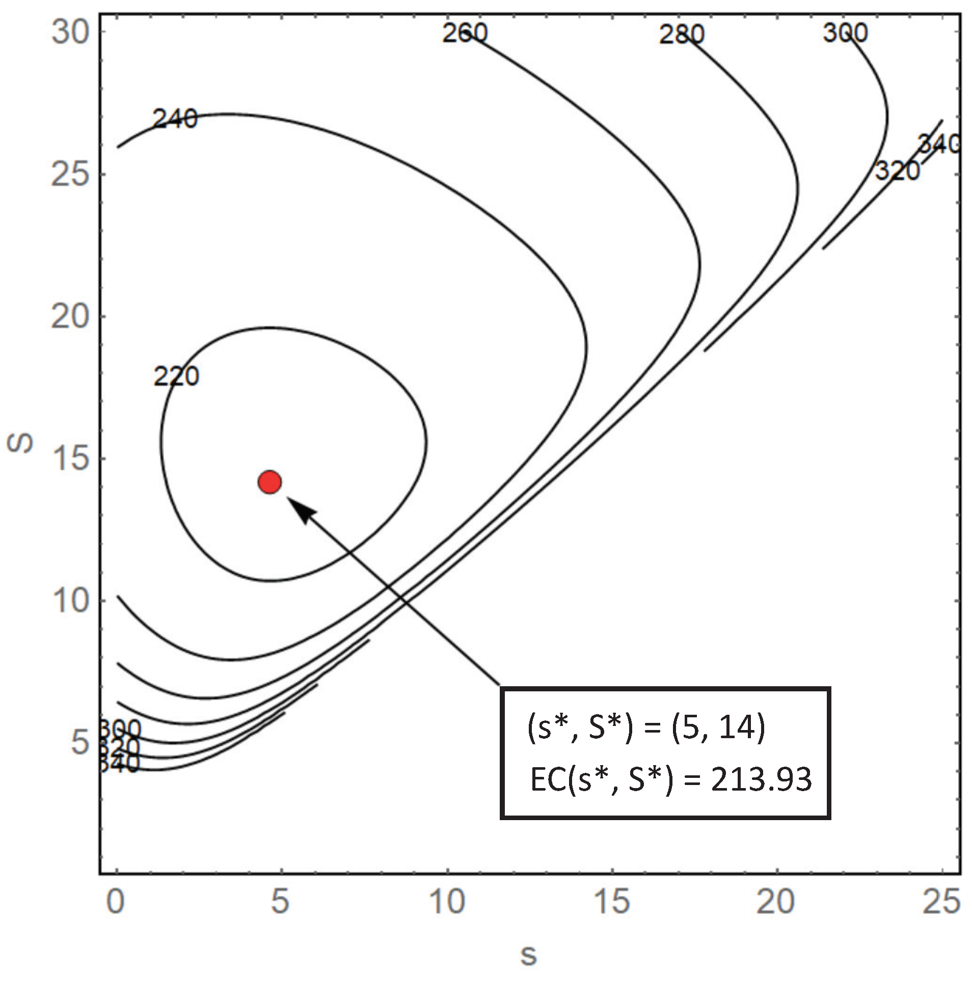
5.2. The Optimal Policy

The cost function, denoted as $EC(s,S)$, encompasses a complex structure. Consequently, identifying any significant analytical properties proves to be a laborious task. Nevertheless, numerous numerical examples have been examined, including all examples presented in the following section. These examples suggest that the function is convex with respect to s and S. Figure 5 serves as a representative example, where $s^{*}$ and $S^{*}$ represent the optimal values. The optimal search algorithm was executed on an Intel Core i9 processor equipped with 32 GB RAM, utilizing Mathematica version 11 for implementation. The computation was completed in approximately 0.0013754 s. The ‘AbsoluteTiming’ function in Mathematica was employed to measure the computation time.

To determine the optimal policy $(s^{*},S^{*})$ that minimizes the expected cost $EC(s^{*},S^{*})={min}_{s,S}EC(s,S)$, a numerical search method is applied. The method is detailed in Algorithm 1 as follows:

Algorithm 1 Finding Optimal Policy (s*, S*) Algorithm

1: Initialize the value of s.   2: Set $ϵ$ as a small threshold value.   3: Initialize diff with a large value.   4: repeat   5:     Compute $S_s^{*}$ such that $EC(s,S_s^{*})={min}_{S}EC(s,S)$.   6:     With $S_s^{*}$ fixed, compute $s_S^{*}$ such that $EC(s_S^{*},S_s^{*})={min}_{s}EC(s,S_s^{*})$.   7:     Calculate $\mathrm{currentEC}=EC(s,S_s^{*})$.   8:     Calculate $\mathrm{newEC}=EC(s_S^{*},S_s^{*})$.   9:     Update $\mathrm{diff}=|\mathrm{newEC}-\mathrm{currentEC}|$. 10:     if $\mathrm{diff}<ϵ$ then 11:         Set $(s^{*},S^{*})=(s_S^{*},S_s^{*})$. 12:         break. 13:     else 14:         Set $s=s_S^{*}$. 15:     end if 16: until Optimal values are found or $\mathrm{diff}<ϵ$.

5.3. Cost–Benefit Analysis of Controlling Inventory Replenishment Speed: Numerical Examples

This section provides a cost comparison associated with exclusive reliance on either high-speed (high-cost) or normal (low-cost) production modes, against the backdrop of the proposed policy of adjusting production speeds. This numerical study aims to delineate the cost effectiveness of the proposed strategy in contrast to traditional approaches that are limited to singular mode utilization. Through this, this section underscores the significance of strategic production speed adjustment, highlighting its role in reducing operational costs in inventory management.

The models operating exclusively in either high-speed (high-cost) or normal (low-cost) modes are characterized as $(S-1,S)$ queuing–inventory models. For these exclusive operational scenarios, mean performance measures and average operating costs are derived from Equations (38)–(40). This is achieved by setting s to $S-1$ and substituting $\eta$ with the respective production speed parameters (${\beta }_N$ for normal mode and ${\beta }_H$ for high-speed mode). For the comparison, the average operating costs $E{C}_H\left(S\right)$ and $E{C}_N\left(S\right)$ for high-speed (high-cost) and normal (low-cost) modes are, respectively, defined as follows:

$$\begin{array}{c}\hfill E{C}_H\left(S\right)=c_{high}{P}_{on}\left({\beta }_H\right)+c_h{\mathbb{E}}_{sp}(I;{\beta }_H)+c_l\lambda {\chi }_{sp}(0;{\beta }_H)+c_w\mathbb{E}\left(N\right)+\frac{r_H}{K_{sp}(S-1,S;{\beta }_H)},\end{array}$$

(46)

and

$$\begin{array}{c}\hfill E{C}_N\left(S\right)=c_{normal}{P}_{on}\left({\beta }_N\right)+c_h{\mathbb{E}}_{sp}(I;{\beta }_N)+c_l\lambda {\chi }_{sp}(0;{\beta }_N)+c_w\mathbb{E}\left(N\right)+\frac{r_N}{K_{sp}(S-1,S;{\beta }_N)},\end{array}$$

(47)

in which, $P_{\mathrm{on}}\left(\eta \right)={\sum }_{n=0}^{\infty }{\sum }_{k=0}^{S-1}{X}_{on}(n,k;\eta ,S-1,S)$, ${\mathbb{E}}_{sp}(I;\eta )={\sum }_{n=0}^{\infty }{\sum }_{k=0}^{S-1}k{X}_{on}(n,k;\eta ,S-1,S)+S{\sum }_{n=0}^{\infty }{X}_{off}(n,S;\eta ,S-1,S)$, and ${\chi }_{sp}(0;\eta )={\sum }_{n=0}^{\infty }{X}_{on}(n,0;\eta ,S-1,S)$.

In the numerical example, the parameters $r_H$, $c_{high}$, and $c_{normal}$ were varied to assess their impact on the optimal average system operating cost, with all other cost coefficients and parameters held constant. To assess the benefit of adopting the proposed policy, $G_{\max }$ is defined as follows:

$$\begin{array}{c}\hfill G_{\max }=\frac{EC(s^{*},S^{*})-min(E{C}_N\left(S^{*}\right),E{C}_H\left(S^{*}\right))}{min(E{C}_N\left(S^{*}\right),E{C}_H\left(S^{*}\right))}.\end{array}$$

(48)

$G_{\max }$ provides as the maximum potential cost savings achieved by implementing the proposed control policy. It is expressed as a percentage relative to the lower cost of either the normal or high-speed modes.

Table 1. Optimal average operating cost per unit time for varying $r_H$ when other parameters are fixed as $\lambda =2$, $\mu =3$, ${\beta }_N=1.1$, ${\beta }_H=2.2$, $c_h=10$, $c_{normal}=50$, $c_{high}=100$, $c_l=500$, $c_w=1$, and $r_N=100$.

${\mathit{r}}_{\mathit{H}}$	$\mathit{EC}({\mathit{s}}^{*},{\mathit{S}}^{*})$	${\mathit{EC}}_{\mathit{N}}\left({\mathit{S}}^{*}\right)$	${\mathit{EC}}_{\mathit{H}}\left({\mathit{S}}^{*}\right)$	${\mathit{G}}_{\mathbf{max}}$
50	209.412	512.222	219.55	4.62%
100	210.997	512.222	232.767	9.35%
150	212.473	512.222	245.762	13.55%
200	213.864	512.222	258.561	17.29%
250	215.187	512.222	271.186	20.65%
300	216.451	512.222	283.654	23.69%
350	217.667	512.222	295.979	26.46%
400	218.84	512.222	308.176	28.99%
450	219.976	512.222	320.254	31.31%
500	221.077	512.222	332.224	33.46%
550	222.149	512.222	344.094	35.44%
600	223.194	512.222	355.872	37.28%
650	224.214	512.222	367.563	39.00%
700	225.211	512.222	379.175	40.60%
750	226.187	512.222	390.711	42.11%

presents a cost comparison of varying the reactivation cost $r_H$ in the high-speed mode. Notably, $E{C}_N\left(S^{*}\right)$ remains constant regardless of changes in $r_H$, as systems operating solely in normal mode are unaffected by changes in $r_H$. Furthermore, the results indicate an increase in $G_{\max }$ with higher $r_H$ values. This is attributed to the elevated costs incurred by frequent reactivations of the high-speed mode in the high-speed-only model. In contrast, the proposed policy optimizes the threshold, leading to significant cost savings compared to an exclusively high-speed operation.

Table 2. Optimal average operating cost per unit time for varying $c_{high}$ when other parameters are fixed as $\lambda =2$, $\mu =3$, ${\beta }_N=1.1$, ${\beta }_H=2.2$, $c_h=10$, $c_{normal}=50$, $c_l=500$, $c_w=1$, $r_N=100$, and $r_H=200$.

${\mathit{c}}_{\mathbf{high}}$	$\mathit{EC}({\mathit{s}}^{*},{\mathit{S}}^{*})$	${\mathit{EC}}_{\mathit{N}}\left({\mathit{S}}^{*}\right)$	${\mathit{EC}}_{\mathit{H}}\left({\mathit{S}}^{*}\right)$	${\mathit{G}}_{\mathbf{max}}$
50	175.671	512.222	223.631	21.45%
60	183.332	512.222	232.366	21.10%
70	190.982	512.222	241.1	20.79%
80	198.621	512.222	249.831	20.50%
90	206.248	512.222	258.561	20.23%
100	213.864	512.222	267.29	19.99%
110	221.469	512.222	276.016	19.76%
120	229.062	512.222	284.741	19.55%
130	236.643	512.222	293.464	19.36%
140	244.212	512.222	302.185	19.18%
150	251.768	512.222	310.904	19.02%
160	259.313	512.222	319.621	18.87%
170	266.845	512.222	328.337	18.73%
180	274.364	512.222	337.05	18.60%
190	281.87	512.222	345.762	18.48%

shows the impact of varying the operating cost, $c_{\mathrm{high}}$, on the overall system costs. Similar to the previous analysis, $E{C}_N\left(S^{*}\right)$ remains unchanged as the inventory is produced exclusively in the normal mode and is unaffected by changes in $c_{\mathrm{high}}$. A key observation is that $G_{\max }$ consistently stays above 0, underscoring the effectiveness of the proposed model in achieving cost savings. This is achieved by dynamically adjusting the s and S thresholds, enabling the system to operate efficiently under both high-speed and normal modes, as opposed to a high-speed-only model, which would incur higher operational costs.

Table 3. Optimal average operating cost per unit time for varying $c_l$ when other parameters are fixed as $\lambda =2$, $\mu =3$, ${\beta }_N=1.1$, ${\beta }_H=2.2$, $c_h=10$, $c_{normal}=50$, $c_{high}=100$, $c_w=1$, $r_N=100$, and $r_H=200$.

${\mathit{c}}_{\mathit{l}}$	$\mathit{EC}({\mathit{s}}^{*},{\mathit{S}}^{*})$	${\mathit{EC}}_{\mathit{N}}\left({\mathit{S}}^{*}\right)$	${\mathit{EC}}_{\mathit{H}}\left({\mathit{S}}^{*}\right)$	${\mathit{G}}_{\mathbf{max}}$
50	139.649	107.222	208.318	−30.24%
100	155.259	152.222	216.252	−2.00%
150	166.8	197.222	223.259	15.43%
200	176.215	242.222	229.564	23.24%
250	184.273	287.222	235.314	21.69%
300	191.371	332.222	240.614	20.47%
350	197.747	377.222	245.538	19.46%
400	203.555	422.222	250.142	18.62%
450	208.901	467.222	254.472	17.91%
500	213.864	512.222	258.561	17.29%
550	218.503	557.222	262.44	16.74%
600	222.861	602.222	266.13	16.26%
650	226.977	647.222	269.651	15.83%
700	230.878	692.222	273.021	15.44%
750	234.588	737.222	276.252	15.08%

shows that the lost-sales cost parameter, $c_l$, significantly influences the system’s operational costs. Unlike previous scenarios, in this case $E{C}_N\left(S^{*}\right)$ varies with changes in $c_l$, due to the pronounced impact of lost sales in a system operating solely in normal mode. This mode, characterized by slower inventory production, leads to increased occurrences of lost sales.

Notably, at very low $c_l$ values, the normal-only mode proves to be the most cost-effective strategy. This is attributed to the economic feasibility of tolerating customer lost sales over incurring the higher costs associated with switching to the high-speed mode.

However, as $c_l$ surpasses a certain threshold, the proposed model demonstrates superior performance compared to both normal-only and high-speed-only modes. This efficiency is attributed to the model’s ability to dynamically balance operational costs between the two modes, optimizing overall system costs. Particularly in scenarios where managing lost sales cost is critical, the proposed model’s adaptability leads to significant cost savings, underscoring its superiority in effectively handling varying cost conditions.

In conclusion, the analyses conducted across various scenarios affirm the proposed model’s efficacy in reducing system costs. It adeptly balances between high-speed and normal operational modes, leading to significant cost savings. The maximum observed $G_{\max }$ value, exceeding 40%, highlights the model’s substantial cost efficiency over single-mode systems. This underscores the value of the proposed model in operational optimization, as it offers flexibility and adaptability in managing costs within queuing–inventory systems.

6. Concluding Remarks and Future Study

This study focuses on a small supply chain system consisting of a make-to-order production facility and a raw material warehouse. Modeled as an M/M/1 queue linked to inventory, the system operates under a modified (s, S) policy, which dynamically adjusts production speed to maintain optimal inventory levels. The analysis led to the derivation of the stationary joint distribution of unmet demands and warehouse inventory levels in product form. From these results, comprehensive cost models were developed. Numerical search methods indicated that the proposed policy could yield maximum cost savings of up to 42%, significantly enhancing cost efficiency over traditional models.

Recent advancements in queuing–inventory systems research, primarily focusing on customer priority integration and responses to disruptions, have informed this study’s motivation. Despite these advancements, a significant gap in exploring variable inventory production speed within these models was identified. Previous studies have extensively analyzed customer retrials, priority levels, negative customer impacts, and warehouse catastrophes, but the relationship between inventory production speed and inventory levels has not been sufficiently explored. This study introduces a model to optimize this relationship, aiming to facilitate more efficient inventory management strategies.

Future work could introduce several generalizations to render the system more realistic. These might include diversifying probability distributions for inter-arrival and production times, incorporating various customer behaviors such as reneging and balking, and exploring a multi-threshold policy for varying internal production speeds. Such enhancements are intended to address the limitations of the current study and to expand the model’s applicability to more complex and realistic supply chain scenarios.

References

1. Baek, J.W.; Moon, S.K. The M/M/1 queue with a production-inventory system and lost sales. Appl. Math. Comput. 2014, 233, 534–544. [Google Scholar] [CrossRef]
2. Cohen, W.E.; Mahafzah, B.A. Statistical analysis of message passing programs to guide computer design. In Proceedings of the Thirty-First Hawaii International Conference on System Sciences, Kohala Coast, HI, USA, 9 January 1998; IEEE: Manhattan, NY, USA, 1998; Volume 7, pp. 544–553. [Google Scholar]
3. Bozer, Y.A.; McGinnis, L.F. Kitting versus line stocking: A conceptual framework and a descriptive model. Int. J. Prod. Econ. 1992, 28, 1–19. [Google Scholar] [CrossRef]
4. Brynzér, H.; Johansson, M.I. Design and performance of kitting and order picking systems. Int. J. Prod. Econ. 1995, 41, 115–125. [Google Scholar] [CrossRef]
5. Harrison, J.M. Assembly-like queues. J. Appl. Probab. 1973, 10, 354–367. [Google Scholar] [CrossRef]
6. Lipper, E.; Sengupta, B. Assembly-like queues with finite capacity: Bounds, asymptotics and approximations. Queueing Syst. 1986, 1, 67–83. [Google Scholar] [CrossRef]
7. Berman, O.; Kaplan, E.H.; Shevishak, D.G. Deterministic approximations for inventory management at service facilities. IIE Trans. 1993, 25, 98–104. [Google Scholar] [CrossRef]
8. Berman, O.; Kim, E. Stochastic models for inventory management at service facilities. Stoch. Model. 1999, 15, 695–718. [Google Scholar] [CrossRef]
9. Berman, O.; Sapna, K. Inventory management at service facilities for systems with arbitrarily distributed service times. Stoch. Model. 2000, 16, 343–360. [Google Scholar] [CrossRef]
10. He, Q.M.; Jewkes, E. Performance measures of a make-to-order inventory-production system. IIE Trans. 2000, 32, 409–419. [Google Scholar] [CrossRef]
11. He, Q.M.; Jewkes, E.M.; Buzacott, J. Optimal and near-optimal inventory control policies for a make-to-order inventory–production system. Eur. J. Oper. Res. 2002, 141, 113–132. [Google Scholar] [CrossRef]
12. Schwarz, M.; Sauer, C.; Daduna, H.; Kulik, R.; Szekli, R. M/M/1 Queueing systems with inventory. Queueing Syst. 2006, 54, 55–78. [Google Scholar] [CrossRef]
13. Schwarz, M.; Daduna, H. Queueing systems with inventory management with random lead times and with backordering. Math. Methods Oper. Res. 2006, 64, 383–414. [Google Scholar] [CrossRef]
14. Baek, J.W.; Moon, S.K. A production–inventory system with a Markovian service queue and lost sales. J. Korean Stat. Soc. 2016, 45, 14–24. [Google Scholar] [CrossRef]
15. Krishnamoorthy, A.; Anbazhagan, N. Perishable inventory system at service facilities with N policy. Stoch. Anal. Appl. 2007, 26, 120–135. [Google Scholar] [CrossRef]
16. Krishnamoorthy, A.; Lakshmy, B.; Manikandan, R. A survey on inventory models with positive service time. Opsearch 2011, 48, 153–169. [Google Scholar] [CrossRef]
17. Krishnamoorthy, A.; Viswanath, N.C. Stochastic decomposition in production inventory with service time. Eur. J. Oper. Res. 2013, 228, 358–366. [Google Scholar] [CrossRef]
18. Saffari, M.; Asmussen, S.; Haji, R. The M/M/1 queue with inventory, lost sale, and general lead times. Queueing Syst. 2013, 75, 65–77. [Google Scholar] [CrossRef]
19. Zhao, N.; Lian, Z. A queueing-inventory system with two classes of customers. Int. J. Prod. Econ. 2011, 129, 225–231. [Google Scholar] [CrossRef]
20. Benny, B.; Chakravarthy, S.; Krishnamoorthy, A. Queueing-inventory system with two commodities. J. Indian Soc. Probab. Stat. 2018, 19, 437–454. [Google Scholar] [CrossRef]
21. Mathew, N.; Joshua, V.; Krishnamoorthy, A. A Queueing Inventory System with Two Channels of Service. In Proceedings of the International Conference on Distributed Computer and Communication Networks, Moscow, Russia, 14–18 September 2020; pp. 604–616. [Google Scholar]
22. Krishnamoorthy, A.; Shajin, D. Stochastic decomposition in retrial queueing inventory system. In Proceedings of the 11th International Conference on Queueing Theory and Network Applications, Wellington, New Zealand, 13–15 December 2016; pp. 1–4. [Google Scholar]
23. Krishnamoorthy, A.; Benny, B.; Shajin, D. A revisit to queueing-inventory system with reservation, cancellation and common life time. Opsearch 2017, 54, 336–350. [Google Scholar] [CrossRef]
24. Chakravarthy, S.; Shajin, D.; Krishnamoorthy, A. Infinite Server Queueing-Inventory Models. J. Indian Soc. Probab. Stat. 2020, 21, 43–68. [Google Scholar] [CrossRef]
25. Liu, Z.; Luo, X.; Wu, J. Analysis of an M/PH/1 retrial queueing-inventory system with level dependent retrial rate. Math. Probl. Eng. 2020, 2020, 4125958. [Google Scholar] [CrossRef]
26. Jeganathan, K.; Vidhya, S.; Hemavathy, R.; Anbazhagan, N.; Joshi, G.P.; Kang, C.; Seo, C. Analysis of M/M/1/N stochastic queueing—Inventory system with discretionary priority service and retrial facility. Sustainability 2022, 14, 6370. [Google Scholar] [CrossRef]
27. Melikov, A.; Poladova, L.; Edayapurath, S.; Sztrik, J. Single-Server queuing–inventory Systems with Negative Customers and Catastrophes in the Warehouse. Mathematics 2023, 11, 2380. [Google Scholar] [CrossRef]
28. Ozkar, S.; Melikov, A.; Sztrik, J. Queueing-Inventory Systems with Catastrophes under Various Replenishment Policies. Mathematics 2023, 11, 4854. [Google Scholar] [CrossRef]
29. Takagi, H.; Tarabia, A.M.K. Explicit Probability Density Function for the Length of a Busy Period in an M/M/1/K Queue. In Advances in Queueing Theory and Network Applications; Yue, W., Takahashi, Y., Takagi, H., Eds.; Springer: New York, NY, USA, 2009; pp. 213–226. [Google Scholar] [CrossRef]
Figure 1. The proposed production–inventory system.
Mathematics 12 00194 g001
Figure 2. The schematic diagram of the proposed model.
Mathematics 12 00194 g002
Figure 3. Sample path of the proposed model.
Mathematics 12 00194 g003
Figure 4. Sample path of the modified model.
Mathematics 12 00194 g004
Figure 5. Contour plot of E C ( s , S ) with respect to s and S when λ = 2 , μ = 3 , β N = 1.1 , β H = 2.2 , c h = 10 , c n o r m a l = 50 , c h i g h = 100 , c l = 500 , c w = 1 , r N = 100 and r H = 200 .
Mathematics 12 00194 g005