Hub-and-Spoke Network Optimization with Flow Delay Cost: The Case of Goods Delivery on Urban Logistics Networks in Eastern China

Abstract

With respect to a traditional point-to-point (P-P) network, a hub-and-spoke (H-S) network not only uses a smaller number of links/paths but also utilizes the scale economy advantage on consolidated flows on hub–hub links and at hubs. However, the inevitable delays through hubs have always been a critical concern. Therefore, this paper develops an H-S model considering flow delay costs and applies the model to a logistics case in Eastern China. The integer quadratic term in the model’s objective function is linearized using the algebraic method. Our model is applied to develop an H-S network for its 13-node express package delivery operation, using the particle swarm optimization (PSO) algorithm. The results show using the H-S can save more than 14.1% of the total cost annually. The model also provides an applied case to the H-S configuration, especially for urban express delivery logistics in China.

1. Introduction

Designing an optimal transportation network has always been a difficult yet strategic task for logistics firms [1,2]. While many network configurations are possible in theory and have been implemented in practice with various pros and cons, two contrasting networks are worthy of comparison. One is the traditional point-to-point (P-P) network, which connects one node to all other nodes directly in the system and often assumes all nodes and links are similar in supply, demand, and capacity. While the P-P network aims to serve all origin and destination pairs directly by avoiding trip transfers or stops, the P-P network inherits some fundamental operational problems, such as low distribution efficiency, frequent sorting and storage at nodes, empty returns due to flow imbalance on links, and cost burdens and limited capacities on minor links and at small nodes. Moreover, the P-P network normally requires greater total system costs, including fixed, operating, and maintenance costs, due to all the O-D pairs being served while many small O-D pairs may not have enough trips or some trips may not exceed a threshold. The other is the hub-and-spoke (H-S) network, which recognizes the hierarchical nature of nodes, links, and paths and utilizes large important nodes and links as hubs and hub–hub (H-H) links to better serve small nodes or non-hubs and hub–spoke (H-S) links. While the H-S network can support some point–point flow movement, its main feature is to move O-D flows through hubs and H-H links so that their scale economy effect can be realized to save costs. As such, fewer direct links and trips are needed while additional sorting, transfer, and stop-over capacities are needed at hubs and on H-H links. Fewer direct connections and more hub transfers may result in higher overall system costs for H-S networks. Therefore, the H-S network can enable logistics firms to reduce costs and improve their business performance.

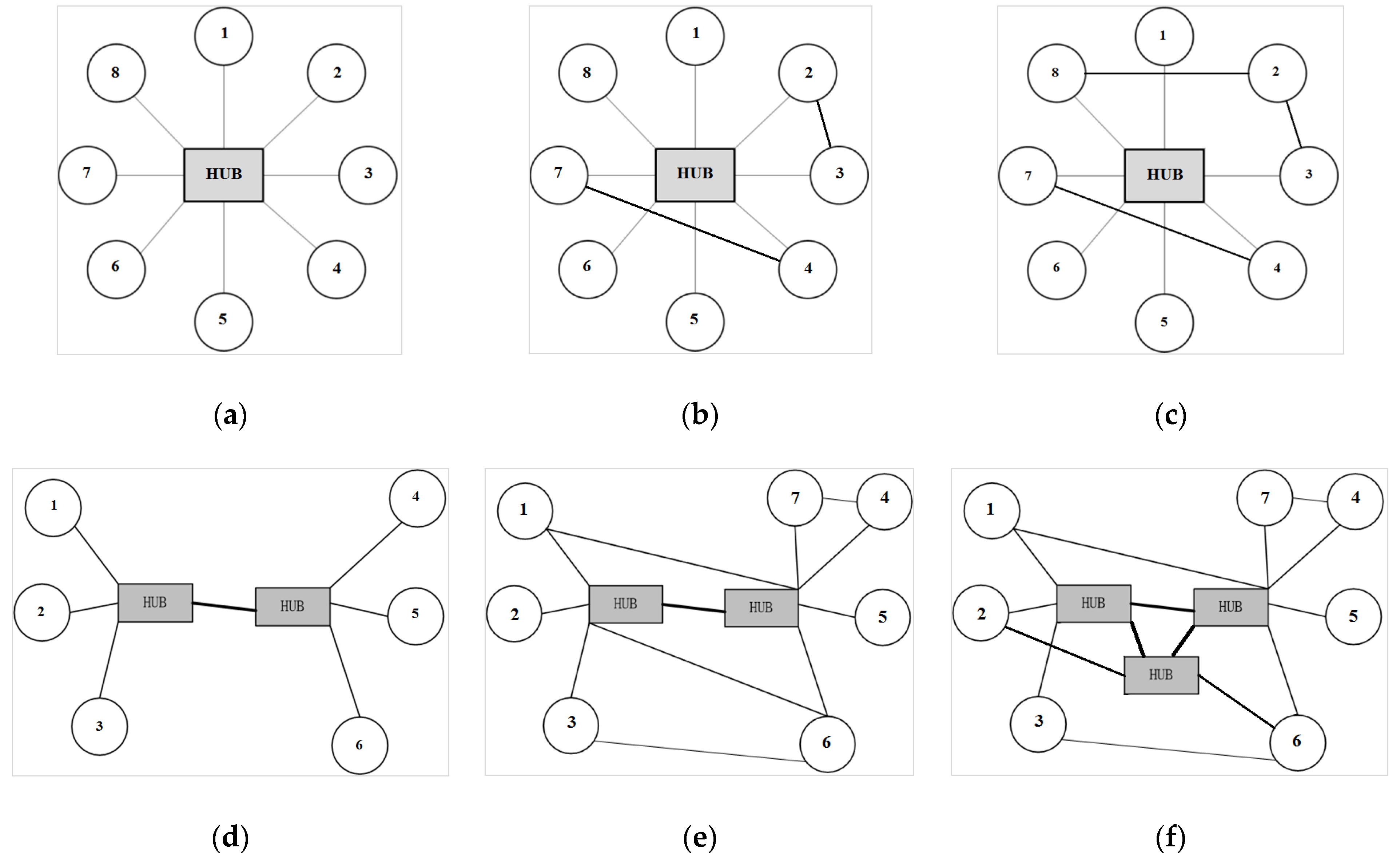
The current research on H-S network design largely focuses on single-hub location and allocation for any O-D pair; that is to say, the non-hub nodes in the network can only be connected to one hub node so the flows between non-hubs (N-N) can only be transferred via the single hub node, hence avoiding direct N-N links or flows while making flows concentrated at hubs and on H-H links. In particular, the number of hubs and their locations in the network are the key factors affecting the operational efficiency of the entire H-S network [3]. At present, most of the logistics firms in China design their H-S networks regarding the hub locations and non-hub allocations based on personal experience and local government regulations in transportation policies and/or urban planning. Compared with the increased transportation cost for operating more links and offering sorting at all nodes in a P-P network, the flow delay costs in the H-S network are often ignored. Today, as lean and green logistics operations are becoming the new normal, and in order to keep a competitive advantage, an increasing number of logistic firms have become more sensitive to transportation costs by strategically adopting the H-S network. Lean implementation positively influences the implementation of sustainability practices for supplier selection and production [4].

With respect to a traditional point-to-point (P-P) network, a hub-and-spoke (H-S) network not only uses a smaller number of links/paths but also utilizes the scale economy advantage on consolidated flows on hub–hub links and at hubs. However, the inevitable delays through hubs have always been a critical concern. The core research question of the paper is how to reduce the total cost of the logistics company by optimizing the H-S network design while considering the flow delay cost and improving the operational efficiency of the logistics network. Following [2], this paper introduces the concept of flow delay cost into the hub location and network design problem as an integral part of the total transportation cost and verifies its practical value through cases. The structure of this paper is as follows: after the introduction in Section 1, Section 2 provides a concise review of the relevant literature on the H-S network. Section 3 describes the concepts of the H-S network. Section 4 proposes an optimized H-S network model considering the flow delay cost at hubs. Section 5 applies the model to the SF firm’s highway network covering 13 prefecture-level cities in the Jiangsu Province, China, using the PSO algorithm to obtain the optimal H-S network and compares the results against the SF’s existing network structure and outcome. Section 6 summarizes and concludes this paper.

2. Literature Review

O’Kelly (1987) introduced the concept of a hub-and-spoke network and proposed a quadratic integer model to locate p hubs for single-hub location and allocation under total transportation cost minimization [5]. Alumur et al. (2008) summarized the literature on single- and multiple-hub location and allocation and network design considering fixed costs, capacities, and coverage [3]. Commemorating the twenty-five years of hub research, Campbell and O’Kelly (2012) provided a comprehensive review of the hub location and network design problem, including model formulations, scale economies, location and allocation schemes, solution algorithms, and application domains and issues [2]. The review also pointed out important future hub research issues and flow delay cost is one of them.

First, different approaches can be taken to solve the same kind of problem. Along with many hub models and location and allocation schemes developed over the past three decades, various solution algorithms have also been developed and implemented. Zheng et al. (2017) proposed a mixed-integer linear programming model, factoring in ship-operating and container-handling costs, and conducted a numerical simulation to test the effectiveness of the model [6]. Devika Kannan et al. (2023) proposed a multi-objective mixed-integer programming (MOMIP) model for configuring an RL network design; it incorporates multiple products, multiple recovery facilities, multiple processing technologies, and a selection of vehicle types [7]. In solving the single-location–allocation model, Aloullal et al. (2023) considered time as a new dimension in the hub location-routing problem, and it employed a specially designed meta-heuristic that combines relax-and-fix, local branching, and variable neighborhood descent techniques for problem-solving [8].

Second, when solving practical problems, there are many factors that need to be considered, and different scholars have different focuses. Alkaabneh et al. (2019) considered a hub-and-spoke network design problem with inter-hub economies of scale and hub congestion and proposed an optimal design of hub-and-spoke networks with nonlinear inter-hub economies of scale and congestion at hub locations [9]. Zhou et al. (2022) designed an H-S network with differentiated services, allowing clients to choose their preferred service levels, while considering multiple transportation modes, with environmental parameters and economies of scale incorporated into the modeling process [10]. Zhou et al. (2023) proposed an H-S network design (HSND) for container shipping in inland waterways based on the tree-like river structure [11].

Third, the hub location and network design problem considering hub and H-H link capacities has been studied as well with various models and/or solution methods reported [12,13,14]. Guan et al. (2018) develop a learning-based probabilistic tabu search to solve the uncapacitated single allocation hub location problem (USAHLP) [15]. Özgün-Kibiroğlu et al. (2019) used the particle swarm optimization (PSO) algorithm to solve the capacitated hub location and allocation model [16]. Najy et al. (2020) considered a novel and more realistic variant of the uncapacitated hub location problem where both flow-dependent economies of scale and congestion considerations are incorporated into the multiple-allocation version of the problem [17]. Daneshfar (2024) et al. proposed an improved version of the discrete laying chicken algorithm (IDLCA) that utilizes noun-based filtering to reduce the number of features and improve text classification performance [18].

Fourth, variations of the hub location and network design model considering congestion, reliability, and other normal and abnormal specifics have also been explored in the literature, for example, flow congestions at the hubs by [19,20] and failure at one or more hubs by [21,22,23]. Karimi-Mamaghan et al. (2020) modeled a single-allocation multi-commodity H-S network problem through a bi-objective mathematical model, considering the congestion in both hubs and connection links [24]. Bütün et al. (2021) tackled H-S network design in the liner shipping sector, introducing a capacitated directed cycle hub location and cargo routing problem under congestion [25]. The experiments show that the network design can be highly influenced by scale economies in mainline vs. feeder transportation costs, the port locations and hinterland flows, and congestion at the hub ports. The hub failure problem viewed from the system reliability perspective was considered by [26,27,28]. Congestion is one of the important reasons for causing delays.

Finally, it is necessary to consider which kind of network structure should be chosen when designing the network. A point-to-point network also has the advantages that the H-S logistics network cannot replace. Reza Lotfi et al. (2021) examine several logistics network designs and evaluate their performance for cost, quality, delivery, flexibility, and resilience [29]. They point out that each network has its strengths: a hub-and-spoke network has economies of scale to reduce delivery costs and routing flexibility to mitigate the effects of disruptions; a cross-docking network provides lower inventory cost; and a pick-up and delivery network provides lower delivery times. They deem that considering a hybrid logistics model in situations where firms need to emphasize cost and resilience.

Two important efforts can be found in the current hub location and network design research. One effort is directed to develop more efficient algorithms to solve larger H-S problems faster. The other effort is on the hub model and network design for different transportation application domains. Few scholars, however, have studied the flow delays and the corresponding costs intrinsic to the H-S network structure. Zhou et al. (2023) proposed a hub-and-spoke network design (HSND) for container shipping in inland waterways based on the tree-like river structure [11]. Then, they determined the optimal hub location, branch port allocation, and fleet deployment, aiming to minimize the total cost of ships, transport, and transport. Considering a multimodal hub-and-spoke transportation network for emergency relief schedules, Li et al. (2023) established a mixed-integer nonlinear programming (MINLP) model considering multi-type emergency relief and multimodal transportation. The model is a bi-objective one that aims to minimize both transportation time consumption and transportation costs [30].

Regarding congestion, there have been scholars conducting related studies but they were concentrated in certain fields, such as aviation and container shipping. Santos et al. (2017) suggested airline companies consider delay problems as routine operations [31]. Sismanidou et al. (2022) revealed a significant correlation between delayed incoming flights and departure delays, offering valuable insights for policies aimed at mitigating airport and network congestion [32]. Huang et al. (2022) investigated an extended container shipping hub-and-spoke network design problem (HSN), considering the failure and congestion of hubs; they developed a 0–1 nonlinear programming model for minimizing the transportation cost [33]. Additionally, congestion and delay may affect service performance and the choice of network structure. Delay problems can be eased by re-designing network structures [34,35,36,37]. Lange et al. (2023) considered a location–allocation–routing problem, postulating that queueing problems result from limited capacities, where congestion occurs [36]. Ashish (2018) pointed out that there were many causes of delay, which could be reduced according to the characteristics of the airport [38]. Yazdi et al. (2017) demonstrated that a baggage fee policy may have a limited effect on alleviating the delays experienced by airlines. [39]. Chen et al. (2021) extended the research on East Asian airports by emphasizing the importance of network attributes in determining flight delays [40].

Few scholars considered flow delay problems when designing H-S logistics network structure, or focused studies on delay costs. Therefore, this paper starts from network structure, and focuses on studying the influence of delay problems on network structure, in the hope of realizing the purpose of improving earnings and enhancing network stability via optimizing network structure.

3. Network Typologies and Flow Delay Cost

3.1. Hub-and-Spoke Network (H-S Network)

According to O’Kelly (1987) and Campbell and O’Kelly (2012), the H-S network can take on quite many configurations, some of which are shown in Figure 1 [5,18]. The simplest H-S network in Figure 1a is also called a star network, in which one hub connects trips and transfers flows for all O-D pairs. Such an H-S network uses minimal links to serve all O-D pairs with the flow concentration at the hub, but once the hub fails, the network fails. Some slight variations to this simple configuration are shown in Figure 1b,c. H-S networks with the location of two or more hubs and multi-allocations with or without non-hub-to-non-hub N-N links are given in Figure 1d–f.

The single-hub H-S network structure is unique because of its simplicity and largely relying on the sole hub. The hub node distributes all or most of the traffic volumes in the network with non-hub nodes transferring through the hub. In the multi-hub H-S network structure, at least two hubs are consolidating and transferring flows, which may be through one hub, two hubs, or more hubs for O-D pairs. Regardless of whether there are one or more hubs in an H-S network, the non-hub nodes can be either allocated to only one hub, hence single-allocation, or to more than one hub, hence multi-allocation. In general, single-hub single-allocation H-S networks are the simplest while multi-hub multi-allocation networks, allowing N-N links, are more complex in network configurations and flow assignments.

The single-hub H-S network structure is easy to connect, relatively easy to manage and maintain, and has strong scalability. The network has a relatively low delay time and a low transmission error. However, this network has the problem of poor simultaneous sharing ability and a low utilization rate of communication lines. The multi-hub H-S network structure has high reliability and strong scalability. The network can be built into a variety of shapes, using a variety of communication channels, and a variety of transmission rates but the network structure is complex, high-cost, and not easy to maintain.

The single-hub location–allocation H-S network is mainly used in small-scale operations in terms of the number of links connected, service areas covered, or traffic volumes served. With all flows going through the single hub, flow congestion at the hub can easily be overwhelmed, especially during peaks. However, with the multi-hub location single-allocation H-S network, O-D flows can be assigned in a more balanced way as additional hubs can transfer otherwise more concentrated flows, this is especially so if the multiple allocation of a non-hub node to more than one hub is allowed. Therefore, a multi-hub location and multi-non-hub allocation H-S network can in general serve larger areas with more O-D pairs with less congestion. Further, if non-hub nodes are allowed to be connected without their O-D flows passing through any hub, the single-hub and multi-hub location and allocation H-S networks actually incorporate partial P-P configurations. n may be divided by subheadings. It should provide a concise and precise description of the experimental results, their interpretation, and the experimental conclusions that can be drawn.

3.2. Flow Delay Cost

In urban freight logistics, the dominant mode of transportation is the highway with commercial trucks as the primary vehicles. If the H-S network is used, the inherent flow delay cost is shown in Figure 2. The flow from origin i to destination j can go directly from i to j or from i through hubs at k and l to j. Clearly, i to j directly is like an O-D link in a P-P network and i to k and l to j is like an O-D path in an H-S network with one (if k or l is a hub) or two hubs (if k or l are both hubs). Evidently, link ij from i to j is shorter than the path ij consisting of N-H link ij, H-H link kl, and N-H link lj, indicating that under the same traffic conditions, it takes a longer distance or time; hence, it is more costly for a truck to go from i to j through hubs k and l. The difference between the two in time, distance, or corresponding cost is regarded as the flow delay cost. This paper takes the flow delay cost as an important part of the total transportation cost in hub location and network design.

4. Model Formulation

4.1. Assumptions and Notations

Our hub location and network design model considering flow delay cost is based on some basic assumptions: (i) Assuming the number of all nodes in the logistics network is n and the number of hub nodes is p, the traffic volume and distance for each O-D pair are set as fixed values for the modeling purpose. (ii) Link and hub capacity constraints are not considered. Each non-hub node can only be connected to one hub, hence single-allocation. The p hubs are fully connected, yet each O-D flow can only go through one or two hubs. (iii) There is a flow or distance-based unit cost for each link ij and there is a discount for the H-H links to reflect the scale economy due to flow concentration. The rest of the model notations are given in

Table 1. Notations for key model parameters and variables.

n:	Total number of nodes in the network;
p:	The number of hub nodes to be located;
$W_{ij}$:	Total transportation flow from node i to node j, where $W_{jj}$ = 0;
$\alpha$:	Discount factor to transportation cost on H-H links due to flow concentration;
$D_{ij}$:	Distance between node i and node j;
$D_{ik}$:	Distance between node i and hub k;
$D_{jl}$:	Distance between node j and hub l;
$D_{kl}$:	Distance between hub k and hub l;
$C_{ij}$:	Unit cost for flow and distance between node i and node j;
$C_{ik}$:	Unit cost for flow and distance between node i and hub k;
$C_{jl}$:	Unit cost for flow and distance between node j and hub l;
$C_{ij}$:	Unit cost for flow and distance between hub node i and hub j;
$Z_{ik}$:	If non-hub node i is connected to hub k, then $Z_{ik}$ = 1, otherwise $Z_{ik}$ = 0;
$Z_{jl}$:	If non-hub node j is connected to hub l, then $Z_{jl}$ = 1, otherwise $Z_{jl}$ = 0;
$Z_{ij}$:	If $Z_{ik}$ and $Z_{jl}$ exist, then $Z_{ij}$ = 1, otherwise $Z_{ij}$ = 0;
$Z_k$:	If node k is the hub, then $Z_k$ = 1, otherwise $Z_k$ = 0.

.

In the H-S network, there are n nodes, if p nodes are considered as hubs, then the remaining n-p nodes are non-hub points. According to the basic assumption (ii), set the regular transportation route as i→k→l→j, where node k and node l are hubs.

4.2. Model Formulation

Based on suggestions from Campbell and O’Kelly (2012), the modified model of the multi-hub location and single-hub allocation in O’Kelly (1987), by considering the flow delay cost [2,5], our model #1 is

$$Min:\sum _{i=1}^n\sum _{j=1}^n{W}_{ij}\left(\sum _{k=1}^n{Z}_{ik}{C}_{ik}{D}_{ik}+\sum _{l=1}^n{Z}_{jl}{C}_{jl}{D}_{jl}+\alpha \sum _{k=1}^n\sum _{l=1}^n{Z}_{ik}{Z}_{jl}{C}_{kl}{D}_{kl}\right)$$

(1)

$$Subjectto\sum _{k=1}^n{Z}_{ik}=1$$

(2)

$$\sum _{k=1}^n{Z}_k=p,$$

(3)

$$\left(n-p+1\right)Z_k\ge \sum _{i=1}^n{Z}_{ik},$$

(4)

$$Z_{ik},Z_{jl}{,Z}_{ij},Z_k\in \left\{\mathrm{0,1}\right\},i,j,k,l\in \left\{\mathrm{1,2},\dots ,n\right\},$$

(5)

The objective function (1) contains two parts. The first part is the transportation cost between non-hub nodes and hub nodes and between hub nodes:

$$Z_1=\sum _{i=1}^n\sum _{j=1}^n{W}_{ij}\left(\sum _{k=1}^n{Z}_{ik}{C}_{ik}{D}_{ik}+\sum _{l=1}^n{Z}_{jl}{C}_{jl}{D}_{jl}+\alpha \sum _{k=1}^n\sum _{l=1}^n{Z}_{ik}{Z}_{jl}{C}_{kl}{D}_{kl}\right)$$

(6)

The second part is the delay cost in the logistics network:

$$Z_2=\sum _{i=1}^n\sum _{j=1}^n{W}_{ij}{C}_{ij}\left(\sum _{k=1}^n{Z}_{ik}{D}_{ik}+\sum _{l=1}^n{Z}_{jl}{D}_{jl}+\sum _{k=1}^n\sum _{l=1}^n{Z}_{ik}{Z}_{jl}{D}_{kl}-Z_{ij}{D}_{ij}\right)$$

(7)

Formula (1) shows that the delay cost is the research object to find the minimum target value under the premise of satisfying the many constraints. Formula (2) is to ensure the single-hub allocation, that is, a non-hub node can only be connected with one hub. The i is the non-hub node, and k is the hub node. Formula (3) is to ensure the multi-hub location, which means to find the best locations for p hubs. Formula (4) means that a hub node can only be connected to a non-hub node if it opens the service function or if a hub station is built at a certain node. Only when the construction of the hub is completed at k can node i be served by node k. Formula (5) means that the variables are both 0–1 variable constraints. Formula (6) details the transportation cost between non-hub nodes and hub nodes and between hub nodes. Formula (7) shows the delay cost in the logistics network.

4.3. Algebraic Linearization

Please note that the model (1)–(5) is still a 0–1 mixed-integer quadratic model due to two $Z_{ik}{Z}_{jl}$ items in the objective function and, hence, NP is hard to solve exactly for large problems. For example, when n = 10, this integer quadratic term will require cycle calculations f04 times, and the duration of cycle calculations will increase with the increase in the number of nodes n. Therefore, it is necessary to linearize the integer quadratic term so as to reduce the number of cycles and accelerate the calculation process. The solution here is to introduce a 0–1 decision variable to represent hub connections and linearize the quadratic term $Z_{ik}{Z}_{jl}$ using the algebraic approach suggested in Shen (1996, 2018) [41,42], defined as follows:

$$Z_{kl}=\left\{\begin{array}{c}1,\mathrm{h}\mathrm{u}\mathrm{b}\mathrm{n}\mathrm{o}\mathrm{d}\mathrm{e}k\mathrm{i}\mathrm{s}\mathrm{c}\mathrm{o}\mathrm{n}\mathrm{n}\mathrm{e}\mathrm{c}\mathrm{t}\mathrm{e}\mathrm{d}\mathrm{t}\mathrm{o}\mathrm{h}\mathrm{u}\mathrm{b}\mathrm{n}\mathrm{o}\mathrm{d}\mathrm{e}l\\ 0,\mathrm{h}\mathrm{u}\mathrm{b}\mathrm{n}\mathrm{o}\mathrm{d}\mathrm{e}k\mathrm{i}\mathrm{s}\mathrm{n}\mathrm{o}\mathrm{t}\mathrm{c}\mathrm{o}\mathrm{n}\mathrm{n}\mathrm{e}\mathrm{c}\mathrm{t}\mathrm{e}\mathrm{d}\mathrm{t}\mathrm{o}\mathrm{h}\mathrm{u}\mathrm{b}\mathrm{n}\mathrm{o}\mathrm{d}\mathrm{e}l\end{array}\right.$$

(8)

A constraint is added:

$$Z_{ik}{Z}_{jl}=Z_{kl}$$

(9)

The final model is

$$Min:Z_1+Z_2$$

(10)

$$Subjectto\left(2\right)–\left(5\right),\left(8\right),\left(9\right)$$

(11)

Formula (10) is the objective function, guaranteeing the minimum transportation cost and the delay cost in the logistics network. Constraint condition (11) indicates that in order to solve the objective function (10), constraint (2) to constraint (5), constraint (8), and constraint (9) are required.

5. Algorithm and Application

There are various kinds of heuristic algorithms. This paper takes five heuristic algorithms as examples to find the solution algorithms suitable for this paper. For the merits of the five heuristics, the comparison results are shown in

Table 2. Comparison of different heuristic algorithms.

Algorithms	Advantages	Disadvantages
Genetic Algorithms	Can be designed in combination with other algorithms, with strong search capability and robustness of the results.	Programming is more complex, searching is slow, and solving is time-consuming.
Taboo Search Algorithm	Can find the global optimum as far as possible, and effectively avoid falling into the dilemma of local optimization.	The solution result and time duration are greatly affected by the initial solution
Simulated Annealing Algorithm	Strong advantage in local search, short solution time.	The disadvantage of global search is obvious, and it is easily affected by the set parameters.
Ant Colony Algorithm	Strong search capability, can be used in combination with other heuristics.	The setting of parameters affects the speed of the solution, the calculation is complicated, the solution time is long, the convergence time is long, and the solution may be a local optimum.
Particle Swarm Algorithm	Fast convergence, less parameter adjustment, more flexible, simple structure, easy to realize.	The solution may be locally optimal, but the dilemma of local optimization can be alleviated through multiple runs.

.

Compared with other heuristic algorithms, particle swarm optimization (PSO) has the characteristics of faster convergence, fewer parameters to be adjusted, a simpler structure, and easier implementation. It can quickly and efficiently select the specified number of hubs. It should be noted that PSO is a heuristic algorithm that may fall into a local optimal solution, so parameter tuning and multiple runs according to the specific problem are required to increase the probability of finding the global optimal solution. In the process of network layout optimization, there are many parameters involved, the solution requires more cycles, and the particle swarm algorithm has the advantages of fast convergence, a fast solution, and it can give the optimization scheme quickly, so this paper chooses to use the particle swarm optimization algorithm to solve the model.

5.1. Particle Swarm Optimization Algorithm

The PSO is an evolutionary algorithm based on swarm intelligence. The PSO is derived from the study of the predatory behaviors of birds, which was proposed by Eberhart and Dr. Kennedy in 1995. The algorithm shares the information obtained by individuals through group activities, searches for solutions from disorder to order, and finally obtains an optimal solution. It has the advantages of a high rate of convergence and flexible parameter adjustment. Özgün-Kibiroğlu et al. (2019) used the particle swarm optimization (PSO) algorithm to solve the hub location problem and also proved the feasibility and advantage of the particle swarm optimization algorithm applied to the hub-and-spoke network structure [16]. In the research range of this paper, the n-dimensional variable $X=(x_1,x_2,\dots ,x_n)$ is set to be the particles, and every particle represents a feasible program. Assuming the solution space is n-dimensional, every particle could be described in two conditions: location $X_i=(x_{i1},x_{i2},{\dots ,x}_{in})$ and speed $V_i=(v_{i1},v_{i2},\dots ,v_{in})$. The detailed process of the PSO algorithm is as below:

The first step is to confirm the hinge node number p and all the node numbers n and to initialize the particle’s location and speed. This paper sets the initial $X_i$ = unifrnd (0, 1, varsize), where the variable varsize represents the matrix size of the decision variable and function unifrnd generates the random number group in continuous uniform distribution within a specified range. This paper sets the initial $V_i$ = zeros (varsize), and the function zeros creates an empty matrix with the specified size.

The second step is to calculate the particle fitness value for evaluation so as to confirm the particle’s individual optimal value and group optimal value. The evaluation standard of this paper is composite cost; with the purpose of minimizing the composite transport cost. The fitness function code is ${[cost}_i,{sol}_i]=costfunction(X_i)$, wherein $costfunction$ is a self-defining function, used to output and store the fitness value calculation result. $costfunction=@\left(xhat\right)mycost(xhat,model)$, wherein the $mycost$ main file includes the expression of the fitting function and provides the output in the form of a function. According to the models in this paper, the fitness function expressions are ${cost1}_{ij}={c\ast w}_{ij}{(z}_{ik}\ast d_{ik}+z_{jl}\ast d_{jl}+{\alpha \ast z}_{kl}\ast d_{kl})$ and ${cost2}_{ij}=c\ast w_{ij}\ast {z_{ik}\ast z_{jl}\ast z}_{kl}\ast (d_{ik}+d_{jl}+d_{kl}-d_{ij})$. The total transport cost is the sum of $cost1$ and $cost2$, respectively, where i, j, k, and l are set up differently, with each node having a number, i < j, and k, l being hinge nodes. Every particle is moving towards the optimal solution according to its current speed and its experience.

The third step is to update the particle’s location and speed. The updated rules are as follows: $v_{ik+1}=w_k{v}_{ik}+c_1{r}_1\left({pbest}_{ik}-x_{ik}\right)+c_2{r}_2({gbest}_{ik}-x_{ik})$ and $x_{ik+1}=x_{ik}+v_{ik+1}$, with a cyclic update. According to article [13], assume $c_1=chi\ast phi1$, $c_2=chi\ast phi2$, and $w_k=chi$, wherein $chi=2/(phi-2+sqr(ph{i}^2-4\ast phi\left)\right)$, $phi=phi1\ast phi2$, and $phi1=phi2=2.05$. If the number of iterations is reached, then output occurs; if it does not reach the iterations, it returns to the second step.

We fixed the number of initial particle swarms at 150 and the number of iterations at 100. Iterations and node numbers could be regulated voluntarily. In addition, in the software that runs the algorithm, the data module could be self-defined. Repeatable operations could be realized via data updates and the re-installation of parameters.

Table 3. Pseudocode for improving particle swarm optimization (PSO) algorithm.

Procedure PSO

for each particle i

Initialize the velocity Vi and position Xi for particle i

Evaluate particle i and set pBest = Xi

end for

gBest = min{pBest}

while not stop

for i = 1 to N

Update the velocity and position of particle i

Evaluate particle i

If fit (Xi) < fit (pBest)

pBest = Xi;

If fit (pBest) < fit (gBest)

gBest = pBest;

end for

end while

print gBest

end procedure

shows the pseudo-codes of the improved PSO algorithm.

We have implemented the algorithm using the MatlabR2021b programming language due to its robust set of libraries for numerical computations and data analysis, which are particularly well suited for the complex calculations required in our study.

5.2. An Application

SF is a private express delivery company engaged in domestic and international packaging, customs declaration, inspection, and quarantine. In March 1993, it was established and headquartered in the Guangdong Province, China. During the early days of the company, it only provided express services in Hong Kong and Guangdong. With consistent quality service, the firm grew and expanded into provinces and cities in the Yangtze River Delta region, then into East China, North China, and Central China, and eventually provided services nationwide. Today, SF has 39 first-level branches and 2600 self-built outlets all over the country, covering 250 major cities and more than 900 county-level cities or towns.

In recent years, the rapid development of the express delivery industry has brought opportunities to the company’s fast growth, especially in Eastern China with several large cities, including megacities like Shanghai. SF built internal subsidiaries and implemented self-management. Taking the Jiangsu Province as an example, SF has opened nearly one thousand last-mile local business outlets and chose Huai’an, Nanjing, and Wuxi as the main transfer and distribution centers (i.e., hub nodes) for the northern, central, and southern regions of the Jiangsu Province. According to their geographical locations, these three hubs serve the whole Jiangsu Province. Other prefecture-level cities basically connect to their respective closest hub nodes to form SF’s three hub locations and single-hub allocation H-S network structure, in which Huai’an connects to “Xuzhou, Lianyungang, Suqian, Yancheng”; Nanjing connects to “Yangzhou and Zhenjiang”; and Wuxi connects to “Taizhou, Changzhou, Suzhou, and Nantong”. However, the flow delay costs, which have been ignored, have become a burden to the firm, especially with the increasing business volume. SF management felt it urgent to reconsider the cost-saving potential for its Eastern China regional operations using a better-designed multi-hub location and single-hub allocation H-S network structure. The central task is to locate more than one and up to four hubs.

The Jiangsu Province is an economically developed region in Eastern China with excellent transportation services and capacities. Each of its major cities is one of the top 100 cities in China with unique strength and can serve as an alternative hub. The company’s express package delivery services are balanced, and the demand is high in all directions without many empty trucks returning. Therefore, each of the 13 prefecture-level cities in the province can be regarded as an alternative hub, namely Nanjing, Wuxi, Xuzhou, Changzhou, Suzhou, Nantong, Lianyungang, Huaian, Yancheng, Yangzhou, Zhenjiang, Taizhou, and Suqian, which are, respectively, labeled as I1 to I13 in Figure 3.

The number of hubs and their locations in an H-S network directly influence the effects of flow concentration on H-H links and their economies of scale. If there are too many hubs, they may dilute the express traffic, resulting in a decrease in the H-H flow discount effects. Otherwise, if there are too few hubs, a high flow concentration may occur at hubs and on H-H links, leading to large delay cost losses and heavy hub operation pressures. Therefore, determining the optimal number of hubs and their locations is an important part of the H-S network design. Currently, there is no single best way to determine the number of hubs for an H-S network. According to Boland et al. (2004), when n = 13, p can be 1, 2, 3, or 4 [43]. When p = 5 or 6, the number of hubs is excessive largely due to the large fixed and operating costs of hubs and, hence, becomes contradictory to SF’s original idea of cost saving [39]. When p ≥ 7, at least one non-hub node connects two hub nodes for multi-hub allocation, which is inconsistent with this study’s assumptions. When p = 1, the hub must be Nanjing, because Nanjing is the capital city of the Jiangsu Province. Therefore, the model application below only considers the cases when p = 2, 3, or 4.

Table 4. Average daily O-D flows between 13 cities in the Jiangsu province, China (kg).

	I1	I2	I3	I4	I5	I6	I7	I8	I9	I10	I11	I12	I13
I1	0	2037	3509	13,829	5312	7238	5127	5225	17,150	1867	10,797	7385	3215
I2	3063	0	2961	10,364	4659	5715	3380	3624	13,205	3236	31,898	8670	1766
I3	4554	1589	0	906	993	711	693	1922	1586	2124	981	836	236
I4	11,288	1040	2841	0	2220	58,830	1283	2051	4434	1581	8573	942	257
I5	79,070	6611	10,388	22,476	0	17,631	20,619	8631	1410	7303	36,614	9630	14,988
I6	13,638	9629	1176	3800	1335	0	2549	1196	1439	7509	8508	2994	1431
I7	1199	332	257	1029	1059	942	0	398	1658	717	5826	205	216
I8	9633	14,402	323	3188	4013	315	9521	0	173	3464	210	213	1287
I9	2205	1199	216	942	257	332	398	1029	0	1658	717	1059	939
I10	9285	4610	779	900	1259	638	770	3105	4496	0	6282	1103	546
I11	45,540	1589	906	993	711	693	1922	1586	2124	981	0	836	236
I12	3464	9521	213	1287	9633	323	107	315	173	3188	4013	0	210
I13	1125	884	507	531	2649	260	689	410	897	462	173	800	0

and

Table 5. O-D distances between 13 cities in the Jiangsu province, China (km).

	I1	I2	I3	I4	I5	I6	I7	I8	I9	I10	I11	I12	I13
I1	0	199	344	159	252	310	305	185	281	101	75	156	259
I2	199	0	514	40	53	103	415	296	239	147	124	129	394
I3	344	514	0	479	575	571	225	218	374	388	396	410	120
I4	159	40	479	0	93	102	415	271	249	107	84	129	364
I5	252	53	575	93	0	99	470	357	281	218	167	197	464
I6	310	103	571	102	99	0	388	328	192	193	184	141	423
I7	305	415	225	415	470	388	0	122	196	292	314	315	172
I8	185	296	218	271	357	328	122	0	130	172	195	192	97
I9	281	239	374	249	281	192	196	130	0	186	211	174	227
I10	101	147	388	107	218	193	292	172	186	0	25	52	269
I11	75	124	396	84	167	184	314	195	211	25	0	77	282
I12	156	129	410	129	197	141	315	192	174	52	77	0	289
I13	259	394	120	364	464	423	172	97	227	269	282	289	0

show the average daily O-D flows and distance matrices for the 13 prefecture-level cities, respectively. The data were obtained from the research department of SF Company. The O-D flow matrix provides a detailed breakdown of the average daily shipment flows between each pair of the 13 prefecture cities within the network. Each cell in the matrix represents the average volume of goods (express packages) that are transported daily from one city to another. The matrix is symmetrical, as the flow from city A to city B is the same as from city B to city A, assuming bidirectional traffic. The distance matrix outlines the average distances between each pair of the 13 cities. Each cell in the matrix indicates the average distance that must be traveled from one city to another, based on the most commonly used transportation routes.

Considering the minor variations of roads in the Jiangsu Province, the transportation rate between any two cities in the Jiangsu Province is set at C level. According to SF’s express delivery cost schedules in the Jiangsu Province, the average transportation cost rate at level is C = 0.03 yuan/kg*km.

6. Results and Analysis

6.1. Main Results

Applying the data in Table 3 to the modified model with the improved PSO algorithm and following the steps in Table 2, we obtained the optimal results corresponding to different p ($=$2, 3, 4) and $\alpha (=0.2,0.4,0.6,0.8,1.0)$ values in

Table 6. Optimal results under different p and α values (CNY).

No. of Cities (n)	No. of Hubs (p)	Hub Location	Selected Hub City (k, l)	α	Transportation Cost (Y1)	Delay Cost (Y2)	Optimal Value (Y1 + Y2)	The Flow at the Hub
13	2	8, 11	Huian Zhenjiang	0.2	2,889,605	335,400	3,225,005	8 (396,392) 11 (870,178)
13	2			0.4	3,112,500	361,272	3,473,772
13	2			0.6	3,335,395	387,144	3,722,539
13	2			0.8	3,558,290	413,016	3,971,306
13	2			1.0	3,621,600	420,364	4,041,964
13	3	4, 11, 13	Changzhou, Zhenjiang, Suqian	0.2	2,216,044	266,640	2,482,684	4 (575,562) 11 (509,820) 13 (196,592)
13	3			0.4	2,530,894	304,524	2,835,418
13	3			0.6	2,845,744	342,408	3,188,152
13	3			0.8	3,160,595	380,291	3,540,886
13	3			1.0	3,475,446	418,174	3,893,620
13	4	4, 9, 11, 13	Changzhou, Yancheng, Zhenjiang, Suqian	0.2	1,871,334	231,998	2,103,332	4 (575,562) 9 (101,728) 11 (479,706) 13 (130,219)
13	4			0.4	2,222,838	275,575	2,498,413
13	4			0.6	2,574,342	319,152	2,893,494
13	4			0.8	2,925,846	362,729	3,288,575
13	4			1.0	3,277,349	406,307	3,683,656

.

The first column shows the number of cities (n = 13) as nodes. The second column shows the number of hubs to be located, p. The third and fourth columns provide the optimal hub locations selected. The fifth column lists the values of discount factor α. Columns six–eight list the optimal O-D transportation costs Y₁, the flow delay cost Y₂, and the total optimal cost $Y_1+Y_2$. For example, for p = 4 and α = 0.8, the optimal objective function value is $Y_1+Y_2$ = CNY 3,288,575 and the four selected hubs are located at I4, I9, I11, and I13, or in cities of Changzhou, Yancheng, Zhenjiang, and Suqian.

To simulate the SF’s current operations, the three hub cities are prefixed at I1, I2, and I8 with the corresponding cities being Nanjing, Wuxi, and Huai’an. The non-hub nodes connecting the hub node Nanjing (I1) are Yangzhou (I10) and Zhenjiang (I11); those connecting the hub node Wuxi (I2) are Changzhou (I4), Suzhou (I5), Nantong (I6), and Taizhou (I12); and those connecting the hub node Huai’an (I8) are Xuzhou (I3), Lianyungang (I7), Yancheng (I9), and Suqian (I13). The overall H-S network configuration is shown in Figure 4d. Simulating current operations using the final model and data in Table 3 and with the SF’s past operations, we set the discount factor at α = 0.8 and applied the PSO algorithm to solve the model. The objective function value is CNY 4,120,494, which is much larger than the optimal objective function value of CNY 3,540,886 when p = 3 and α = 0.8.

Compared with the results from the simulated SF operations when p = 3 and α = 0.2–1.0, we obtained hub cities at I4, I11, and I13 and the corresponding cities are Changzhou, Zhenjiang, and Suqian. The non-hub nodes connecting to the hub node Changzhou (I4) are Wuxi (I2), Suzhou (I5), and Nantong (I6); those connecting to the hub node Zhenjiang (I11) are Nanjing (I1), Yangzhou (I10), Taizhou (I12), and Yancheng (I9); and those connecting to the hub node Suqian (I13) are Xuzhou (I3), Lianyungang (I7), and Huai’an (I8). The optimal objective function values range from CNY 2,482,684 to CNY 3,893,620.

The optimal H-S configurations corresponding to the above results and the rest of the optimal H-S networks are summarized in Figure 4a–c, in which the yellow square represents the hub nodes, and the circles represent the non-hub nodes. Also, the N-H connections are linked by colored lines and the H-H connections are shown by bold black lines.

6.2. Main Analysis

When p = 3 and α = 0.8, the total cost simulated for current operations for SF is CNY 4,120,494 per day on average, while the total cost obtained using the optimized model is CNY 3,540,886 per day, leading to CNY 579,608 savings per day or a 14.1% total cost reduction. Table 6 provides the cost-saving breakdowns for the transportation cost, flow delay cost, and total cost. Savings are in CNY amount and percentages also were summarized in

Table 7. Cost saving breakdowns (in CNY).

p = 3, α = 0.8	$\mathbf{Transportation}\mathbf{Cost}{\mathit{Y}}_1$		$\mathbf{Flow}\mathbf{Delay}\mathbf{Cost}{\mathit{Y}}_2$		$\mathbf{Total}\mathbf{Cost}({\mathit{Y}}_1+{\mathit{Y}}_2)$
Simulated results	3,265,502.5	79.25%	854,991.6	20.75%	4,120,494.1	100%
Modeled results	3,160,595.2	89.26%	380,291.1	10.74%	3,540,886.3	100%
Differences	104,907.3	18.1%	474,700.5	81.9%	579,607.8	100%
		2.55%		11.55%		14.1%
Total Savings by %	3.2%		55.5%		14.1%

.

In comparing simulated results for current operations and modeled optimal results in Table 6, we can find that (i) the modeled results slightly reduced transportation costs by 3.2% and significantly reduced the flow delay cost by 55.5%, which together led to a 14.1% total cost saving; (ii) the modeled results substantially lowered the flow delay cost from 20.75% to 10.74% while not increasing the transport costs much; (iii) further breakdowns of the cost savings show that transportation costs and flow delay costs contribute 18.1% and 81.9%, respectively. In other words, of the 14.1% of the total cost saving, 2.55% was realized through the transportation cost and 11.55% was through the flow delay cost. Please note that the cost saving here is daily and on average. Annual and long-term savings would be tremendous for SF. In general, it is of paramount importance to consider flow delay cost in planning or designing H-S networks.

The optimal results in Table 5 show that if other conditions remain unchanged when the number of hubs p increases up to four, the optimal values of the objective function or the total transportation cost decrease, even with different discount factor α values. This is largely caused by the fixed cost factor yet to be considered. The total fixed cost factor can be easily modeled by adding it to the objective function in the model (13)–(14) as ${FC}_k{Z}_k$ sum over k. The fixed cost is often considered in the literature to include the hub construction cost and the hub trans-shipment cost. Normally, when the total fixed cost estimate is known, the number of hubs can be roughly estimated. The reverse holds as well.

Based on the results in Table 5, if α = 0.8 and ${FC}_1={FC}_2=\cdots {FC}_k=FC$, the total cost is 3,971,306 + 2 $FC$ when p = 2, 3,540,886 + 3 $FC$ when p = 3, and 3,288,575 + 4 $FC$ when p = 4. When the fixed cost satisfies $lowbound\le FC\le CNY\mathrm{252,311}$ with p = 4, the total cost is always the lowest; if $\yen \mathrm{252,311}<FC<CNY\mathrm{430,420}$, the best hub number is p = 3; when $CNY\mathrm{430,420}\le FC\le upperbound$, the optimal hub number is p = 2. Here, the lower and upper bounds are based on actual resource planning for hub fix costs. Figure 5 shows the relations of these bounds and values.

Also, if other conditions remain unchanged, when the discount factor α for H-H flows increases in a certain range, the total transportation cost increases correspondingly as shown in Table 5. However, the value selection of α does not affect the number of hubs and the hub locations, but it does affect the total optimal cost in a simple proportional way.

Moreover, the trans-shipping nature of hubs and the positive scale economy of flow consolidation on H-H links may well offset the flow delay cost to a certain extent, making the H-S network superior to the point-to-point network. This is the single most important reason that most urban logistics firms adopt operations under a full or semi-hub-and-spoke network configuration. However, it is worthwhile here to quickly compare the P-P and H-S networks to gain a general understanding of major influencing factors.

Figure 6 is the P-P network for the 13-city SF logistics operation. Its total system cost conceptually can be thought of as consisting of transportation costs and fixed costs, which can be expressed as

$$Z_{P-P}=\sum _{i=1}^n\sum _{j=1}^n{W}_{ij}{C}_{ij}{D}_{ij}+n{F}_{P-P}$$

(12)

Assuming $F_{P-P}=\frac{FC}{c}$, with c > 1, a simple calculation yields the P-P transportation at CNY 3,963,642. Therefore, when (1) $lowbound\le FC\le \mathrm{C}\mathrm{N}\mathrm{Y}252,311$, the highest total cost is $\mathrm{3,683,656}+4FC$, and it is best to set $p=4.$ In the meantime, when $1<c\le 4.498$, $(\mathrm{3,683,656}+4FC)<\mathrm{3,963,642}+13FC/c$, the H-S is superior to the P-P; when $c>4.498$, the relative advantage of the two network typologies depends on values of the discount factor and the fixed cost; (2) when $\mathrm{C}\mathrm{N}\mathrm{Y}\mathrm{252,311}\le FC\le \mathrm{C}\mathrm{N}\mathrm{Y}\mathrm{430,420}$, the highest total cost is $\mathrm{3,893,620}+3FC$, the lowest total cost is over $\mathrm{2,129,950}+3FC(\alpha =0)$, and the best number of hubs is $p=3$. If $1<c\le 4.582$, $(\mathrm{3,893,620}+3FC)<\mathrm{3,963,642}+13FC/c$, the H-S network is better than the P-P; however, when $c>4.582$, the H-S advantage cannot be determined due to a lack of conditions. (3) When $\mathrm{C}\mathrm{N}\mathrm{Y}\mathrm{430,420}\le FC\le upperbound$, the lowest total cost is over $\mathrm{2,976,238}+2FC(\alpha =0)$ and the optimal number of hubs $p=2$. Because $\mathrm{430,420}<(\mathrm{3,963,642}-\mathrm{2,976,238})/2$, the relative advantage of the two network typologies depends on the values of the discount factor and the fixed cost.

7. Discussion

The model can be improved in many ways, which may be grouped into two broad directions. One includes the technical improvements of the model, including adding fixed cost directly into the objective function, allowing for more than four hubs to be located and/or only one hub to be located, and expanding the discount factor range beyond 0.2–1.0. In each of these improvements, the total H-S costs can be compared with the P-P costs. Also, capacities for city–city links or streets and trans-shipping time or cost at hubs may be considered. Moreover, reliability on links and at hubs and other practical considerations such as speed limits, congestions, situations for less truck-load or empty-truck load, etc., can be built into the model to make it closer to reality. The other direction for improvements may be on operational and policy aspects to take account of the rapid development of the urban logistics industry, especially on the location, construction, safety, and sustainability of the hub nodes and on the long-term, dynamic, and systematic process of building a complex yet efficient H-S network meeting the business needs of the enterprise and the industry, functional planning requirements of the local cities, and economic and social benefits of the society.

8. Conclusions

This research developed a hub-and-spoke network design model based on the seminal quadratic hub location and allocation model by O’Kelly (1987), considering flow delay cost, scale economy, and multiple hub locations with single-allocation [5]. The model was linearized using the algebraic approach suggested by Shen (1996) and solved using the particle swarm optimization for a local urban express delivery company SF in the Jiangsu Province of Eastern China [42]. In addition to the modeled optimal results and corresponding optimal H-S configurations, exploratory discussions on cost savings with respect to SF’s current operations and the effects of hub fixed cost, discount factor, the number of hubs, and P-P configuration are also presented.

The results show that first, the simple algebraic approach in linearizing the quadratic term worked well. The modeled results showed sizable daily savings (14.1%) in the total cost over the simulated results with the hub locations and other parameters from the current operations of SF. The long-term cost savings are considerable. Second, the model can locate up to four hubs at variable locations, with location 11, or Zhenjiang, selected as a hub regardless of the number of hubs to be located (p = 2, 3, or 4), followed by locations 4 and 13, or Changzhou and Suqian, when p = 3 or 4. Locations 8 and 9, or Huanan or Yancheng, were only selected once as a hub when p = 2 or 4, respectively. In general, when the number of hubs increases, the hubs selected are further apart when fewer hubs are to be located and closer when more hubs are to be located. Also, along with more hubs to be located, the total transportation cost decreases. However, the discount factor seems to have no effect on hub locations but it does proportionally affect the total costs. The flow delay cost has a greater impact on the locations of hubs with larger flow trans-shipments or more allocations by smaller and nearby connecting cities. Given that the hub location, construction, maintenance, and flow concentration are the most important parts of any H-S network, considering flow delay cost in H-S planning is highly recommended.