Article

New One-Parameter Over-Dispersed Discrete Distribution and Its Application to the Nonnegative Integer-Valued Autoregressive Model of Order One

by
Muhammed Rasheed Irshad
1,*,
Sreedeviamma Aswathy
1,
Radhakumari Maya
2 and
Saralees Nadarajah
3
1
Department of Statistics, Cochin University of Science and Technology, Cochin 682022, India
2
Department of Statistics, University College, Thiruvananthapuram 695034, India
3
Department of Mathematics, University of Manchester, Manchester M13 9PL, UK
*
Author to whom correspondence should be addressed.
Mathematics 2024, 12(1), 81; https://doi.org/10.3390/math12010081
Submission received: 10 November 2023 / Revised: 17 December 2023 / Accepted: 19 December 2023 / Published: 26 December 2023

Abstract

:
Count data arise in inference, modeling, prediction, anomaly detection, monitoring, resource allocation, evaluation, and performance measurement. This paper focuses on a one-parameter discrete distribution obtained by compounding the Poisson and new X-Lindley distributions. The probability-generating function, moments, skewness, kurtosis, and other properties are derived in the closed form. The maximum likelihood method, method of moments, least squares method, and weighted least squares method are used for parameter estimation. A simulation study is carried out. The proposed distribution is applied as the innovation in an INAR(1) process. The importance of the proposed model is confirmed through the analysis of two real datasets.

1. Introduction

Count data find diverse applications across various fields, such as the frequency of typing errors on a page or the quantity of lice present on the heads of Hindu male prisoners in Cannanore [1]. Count data modeling provides a powerful framework for understanding and analyzing discrete events or occurrences. It allows researchers, policymakers, and organizations to quantify and interpret patterns, identify influential factors, make predictions, and inform evidence-based decision-making. The most typical models for count data are the Poisson and negative binomial distributions. Because of its equi-dispersive character, the Poisson distribution should not be applied when an over-dispersion issue arises. Note that count data commonly exhibit either over-dispersion or under-dispersion, and this has driven the development of more versatile models over the past few decades.
Recall that real data are often over-dispersed. Many researchers have developed mixed Poisson distributions such as the Poisson Weibull distribution [2], Conway–Maxwell–Poisson distribution [3], Poisson transmuted Lindley distribution [4], Poisson transmuted exponential distribution [5], Poisson quasi-Lindley distribution [6], Poisson Bilal distribution [7], Poisson Xgamma distribution [8], Poisson extended exponential distribution [9] and the Poisson generalized Lindley distribution [10].
Moreover, count data are prevalent in numerous applied research domains. Examples include the number of hospital admissions over time, monitoring the number of stock trades per minute or daily transaction volumes in financial markets, and analyzing the number of reported crimes per month in different regions. A nonnegative integer-valued autoregressive process of order one (INAR(1)) is a discrete-time autoregressive model where the current value of the process depends on its previous value and is restricted to take nonnegative integer values. The INAR(1) process with Poisson innovations due to [11] was the pioneering work of INAR(1) processes. But Poisson distribution assumes that the variance is equal to the mean (equi-dispersion). In over-dispersed count data, this assumption is violated, as the variance is larger than the mean. Since [11], many researchers have suggested INAR(1) processes under non-Poisson innovations. Some examples of other innovations are geometric innovations [12], discrete three-parameter Lindley innovations [13], Bell innovations [14], and discrete Bilal innovations [15]. We list also some mixed Poisson innovations, as follows: Poisson–Lindley innovations [16], new Poisson weighted exponential innovations [17], Poisson quasi-Xgamma innovations [18], discrete pseudo-Lindley innovations [19], Poisson transmuted exponential innovations [20], and Poisson generalized Lindley innovations [10].
Lindley distribution has found applications in various fields such as finance, environmental studies, and medical research, among many others. Due to its ability to handle various types of data, Lindley distribution has become a valuable tool in statistical modeling, particularly in situations where traditional distributions may not provide an adequate fit. Researchers have often used Lindley distribution to gain insights into different datasets and make more accurate predictions and inferences. Here, we consider the continuous new X-Lindley (NXL) distribution [21]. It is a novel one-parameter distribution that incorporates the advantages of both Lindley and exponential distributions. It has potential applications in diverse fields such as biology, engineering, astronomy, actuarial science, and medicine. Moreover, this distribution exhibits an elevated risk rate and a diminishing average residual life function.
In this paper, we compound the Poisson and new X-Lindley distributions, resulting in a new one-parameter distribution, which is referred to as the Poisson new X-Lindley (PNXL) distribution. This new one-parameter distribution can handle over-dispersed count data.
The remainder of the paper is structured as follows. In Section 2, the one-parameter PNXL distribution is introduced and its statistical properties are derived. Estimation techniques utilized to estimate the unknown parameter are described in Section 3, and their finite sample performance is evaluated through a simulation study. A new INAR(1)PNXL process is described in Section 4. Two real datasets are analyzed in Section 5 to demonstrate the effectiveness of the suggested distribution. Conclusions are provided in Section 6.

2. Poisson New X-Lindley Distribution

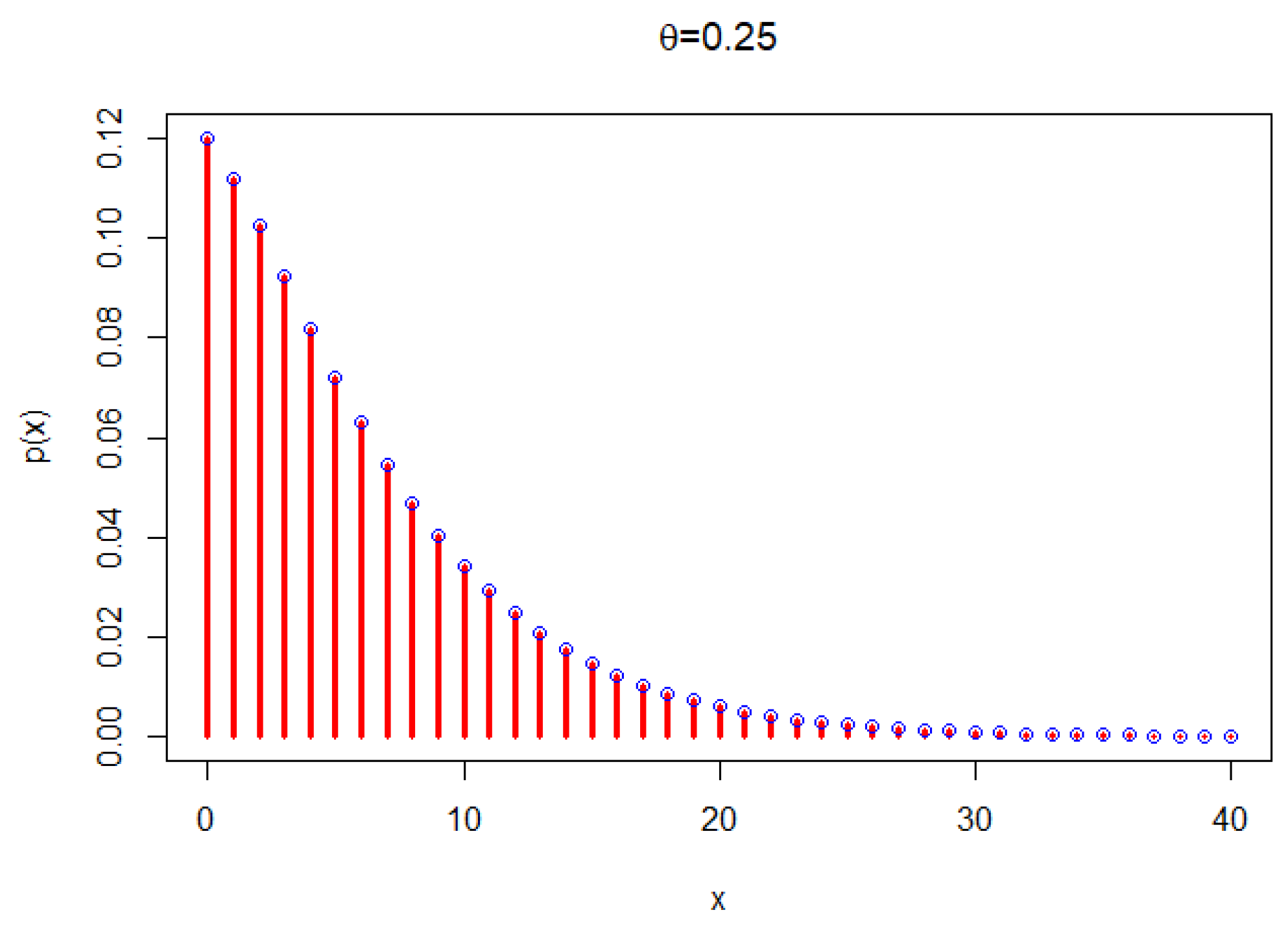
2.1. The Poisson New X-Lindley Distribution and Its Statistical Properties

The NXL distribution is a special case of one-parameter polynomial exponential distribution (NPED) proposed in [22]. The probability density function (pdf) and cumulative distribution function (cdf) of the NXL distribution are given, respectevely, by
p ( x ; θ ) = θ ( 1 + θ x ) e θ x 2 and F ( x ; θ ) = 1 1 2 θ x + 1 e θ x ,
respectively, for x > 0 and θ > 0 . Our suggested one-parameter discrete compound distribution is built on the basis of the NXL distribution. That is, the PNXL distribution is a mixed-Poisson distribution obtained by compounding the Poisson and NXL distributions. Its probability mass function (pmf) is formulated as follows:
Definition 1.
Let X denote a random variable having the PNXL distribution such that X | λ P ( λ ) and λ | θ N X L ( θ ) , where λ > 0 and θ > 0 . The unconditional pmf of X is
p ( x ; θ ) = 0 e λ λ x x ! θ e θ λ ( 1 + θ λ ) 2 d λ = θ ( 2 θ + θ x + 1 ) 2 ( θ + 1 ) x + 2
for x = 0 , 1 , 2 , and θ > 0 .
The corresponding cdf is
F ( x ; θ ) = 2 θ 2 ( 1 + θ ) x + 2 ( 1 + θ ) x 1 + θ 4 ( 1 + θ ) x x 3 2 ( 1 + θ ) x + 2 .
The pmf (1) is log concave since
p ( x + 1 ; θ ) p ( x ; θ ) = 1 + ( 3 + x ) θ ( 1 + θ ) ( 1 + ( 2 + x ) θ )
is a decreasing function in x for all parameter values. Furthermore, p ( x + 1 ; θ ) p ( x ; θ ) < 1 for all x = 0 , 1 , and θ > 0 , so the pmf is unimodal.
Figure 1 plots the pmf of the PNXL distribution.
The survival function (sf) and hazard rate function (hrf) of X are
S ( x ; θ ) = 2 + 3 θ + θ x 2 ( 1 + θ ) x + 2
and
H ( x ; θ ) = θ ( 1 + 2 θ + θ x ) 2 + 3 θ + x θ ,
respectively.

2.2. Moments, Skewness, and Kurtosis

The probability generating function (pgf) of X is
p ( s ; θ ) = θ ( 1 s + 2 θ ) 2 ( 1 s + θ ) 2 .
By replacing s in (2) with e t , the moment-generating function (mgf) of X is
M ( t ) = θ 1 e t + 2 θ 2 1 e t + θ 2 .
Using (3), we obtain the mean, variance, skewness, and kurtosis of X as
E ( X ) = 3 2 θ
and
V ( X ) = 7 + 6 θ 4 θ 2 ,
s k e w ( X ) = 36 2 θ 2 + 13 θ 4 2 ( 7 + 6 θ ) 3
and
k u r t ( X ) = 333 + 612 θ + 304 θ 2 + 24 θ 3 ( 7 + 6 θ ) 2 ,
respectively. The dispersion index (DI) is 1 + 7 6 θ , which implies that the PNXL distribution is over-dispersed.
We see that moments, mean, variance, skewness, kurtosis, and generating functions are all in closed form. The mean and variance decrease as θ increases. The PNXL distribution has positive skewness, which increases as θ increases. Kurtosis decreases as θ approaches 1, and thereafter, it increases.

3. Estimation of Parameters

Various techniques are employed to estimate unknown parameters. We consider the maximum likelihood (ML) method, method of moments (MM), least squares (LS) method, and weighted least squares (WLS) method. We suppose that x 1 , x 2 , , x n is a random sample of size n from the PNXL distribution with ordered values x ( 1 ) < x ( 2 ) < < x ( n ) .

3.1. Maximum Likelihood Estimation

The likelihood function is given by
L ( θ ) = θ 2 n i = 1 n 2 θ + θ x i + 1 ( θ + 1 ) x i + 2
and the log-likelihood function is given by
log L ( θ ) = n log θ n log 2 + i = 1 n log 2 θ + θ x i + 1 ( θ + 1 ) x i + 2 .
The ML estimate (MLE) of θ is obtained by maximizing L ( θ ) or log L ( θ ) with respect to θ . The first derivative of log L ( θ ) with respect to θ is
θ log L ( θ ) = n ( 1 θ x ¯ θ ) θ ( 1 + θ ) + i = 1 n x i + 2 2 θ + θ x i + 1 ,
where x ¯ = 1 n i = 1 n x i . The MLE of θ , denoted by θ ^ M L E , can be obtained by solving θ log L ( θ ) = 0 , provided that the root corresponds to a maximum. We can use the optim function in the R software (R 4.2.1) to obtain θ ^ M L E numerically.

3.2. Method of Moments

The MM estimate (MME) can be obtained by equating theoretical and empirical moments. The MME of θ , denoted by θ ^ M M E , is
θ ^ M M E = 3 2 x ¯ .
Proposition 1.
The MME θ ^ M M E has positive bias.
Proof. 
Note that θ ^ M M E = g x ¯ , where g ( t ) = 3 2 t , t > 0 , is strictly convex. Using Jensen’s inequality, E g X ¯ > g E X ¯ , where g E X ¯ = g 3 2 θ = θ . Hence, θ ^ M M E has positive bias. □

3.3. Least Squares and Weighted Least Squares Estimation

The LS estimate (LSE) of θ , denoted by θ ^ L S E , is obtained by minimizing
Q ( θ ) = i = 1 n F x ( i ) i n + 1 2 .
The WLS estimate (WLSE) of θ , denoted by θ ^ W L S E , is obtained by minimizing
Q w ( θ ) = i = 1 n ( n + 1 ) 2 ( n + 2 ) i ( n i + 1 ) F x ( i ) i n + 1 2 .
The LSE and WLSE can be evaluated numerically using the optim function in the R software (R 4.2.1).

3.4. Simulation Study

This section compares various estimates of θ using simulation. The average absolute biases (biases) and mean square errors (MSEs) were calculated for θ = 0.3, 0.5, 1.2 and n = 50, 100, 200, 250, 500 with replicates N = 1000 :
Bias = 1 N j = 1 N | θ j ^ θ |   and   MSE = 1 N j = 1 N θ j ^ θ 2 ,
where θ j ^ denotes either the MLEs, MMEs, LSEs, or the WLSEs of θ , computed from the jth sample. Table 1 gives the values of biases and MSEs.
We can see that MLE and MME perform almost equally well. For large values of θ , LSE and WLSE do not perform well. For MLEs, there is a noticeable decline in both absolute bias and MSE as the sample size increases. Consequently, the performance of MLE proves to be consistently reliable.

4. The INAR(1) Process with PNXL Innovations

According to [11], as an innovation for INAR(1) processes for over-dispersed count data, we employ the PNXL distribution, which is suitable for over-dispersed data. The INAR(1) process is given by
X t = α X t 1 + ϵ t , t Z ,
where α [ 0 , 1 ) , ϵ t t Z is a sequence of iid nonnegative integer-valued random variables from the PNXL distribution with mean E ϵ t = μ ϵ and variance V ϵ t = σ ϵ 2 . The binomial thinning operator denoted by ‘∘’ is defined as
α X t 1 = j = 1 X t 1 W j ,
where W j j 1 is a sequence of iid Bernoulli random variables with probability of success p. The one-step transition probability matrix for the INAR(1) process is defined by
Pr X t = k | X t 1 = l = i = 1 min ( k , l ) l i α i ( 1 α ) l i Pr ϵ t = k i , k , l 0 .
PNXL innovations are used to propose a new INAR(1) process for over-dispersed data. Let ϵ t t Z follow the PNXL distribution. Then, the one-step transition probability matrix of the corresponding process is
Pr X t = k | X t 1 = l = i = 1 min ( k , l ) l i α i ( 1 α ) l i θ 2 θ + θ ( k i ) + 1 2 ( θ + 1 ) k i + 2 , k , l 0 .
This new process is denoted by INAR(1)PNXL. We can obtain the joint probability function as
f i 1 , i 2 , , i n = Pr X 1 = i 1 , X 2 = i 2 , , X n = i n = Pr X 1 = i 1 Pr X 2 = i 2 | X 1 = i 1 Pr X n = i n | X n 1 = i n 1 = Pr X 1 = i 1 k = 1 n 1 m = 0 min i k , i k + 1 i k m α m ( 1 α ) i k m Pr ϵ k + 1 = i k + 1 m .
The (conditional or unconditional) mean/variance, DI, and autocovariance/autocorrelation (ACF/PACF) at lag k of X t t Z [23] are
E X t | X t 1 = α X t 1 + μ ϵ = α X t 1 + 3 2 θ ,
V X t | X t 1 = α ( 1 α ) X t 1 + σ ϵ 2 = α ( 1 α ) X t 1 + 7 + 6 θ 4 θ 2 ,
E X t = μ ϵ 1 α = 3 2 θ ( 1 α ) ,
V X t = σ ϵ 2 + α μ ϵ 1 α 2 = 7 + 6 ( 1 + α ) θ 4 ( 1 α 2 ) θ 2 ,
D I X t = D I ϵ + α 1 + α = 1 + 7 6 θ + α 1 α ,
γ k = C o v X k , X k + 1 = α k V X t
and
ρ k = C o r r X k , X k + 1 = α k ,
respectively.

4.1. Estimation of INAR(1)PNXL Process

We utilize the conditional maximum likelihood (CML), conditional least squares (CLS), and Yule–Walker (YW) methods. Let x 1 , , x T be the observed count time series of length T.

4.1.1. Conditional Maximum Likelihood

The conditional log likelihood function of the INAR(1) process is
l ( α , θ ) = t = 2 T log Pr X t = k | X t 1 = l = t = 2 T log i = 1 min x t , x t 1 x t 1 i α i ( 1 α ) x t 1 i θ 2 θ + θ ( k i ) + 1 2 ( θ + 1 ) k i + 2 .
The CML estimates of α and θ , denoted by α ^ C M L and θ ^ C M L , respectively, can be obtained numerically by maximizing (6) with respect to α and θ .

4.1.2. Yule–Walker

The YW estimates of α and θ , denoted by α ^ Y W and θ ^ Y W , respectively, can be computed by equating theoretical and empirical moments of the INAR(1)PNXL process, as follows:
α Y W ^ = t = 2 T x t x ¯ x t 1 x ¯ t = 1 T x t x ¯ 2
and
θ Y W ^ = 3 2 ( 1 α Y W ^ ) x ¯ ,
where x ¯ = 1 N t = 1 T x t .

4.1.3. Conditional Least Squares

The CLS estimates of α and θ , denoted by α ^ C L S and θ ^ C L S , respectively, can be obtained by minimizing
Q ( η ) = t = 2 T X t E X t | X t 1 2 = t = 2 T X t α X t 1 3 2 θ 2 ,
as follows
α ^ C L S = ( T 1 ) t = 2 T X t X t 1 t = 2 T X t t = 2 T X t 1 ( T 1 ) t = 2 T X t 1 2 t = 2 T X t 1 2
and
θ ^ C L S = 3 ( T 1 ) 2 t = 2 T X t α ^ C L S t = 2 T X t 1 .

4.2. Simulation of INAR(1)PNXL Process

A simulation study was carried out to assess the performances of CML, CLS, and YW estimates. The biases and MSEs were calculated for the three estimates for α = 0.4 , 0.8 , θ = 0.8 , 3 , and n = 50 , 100 , 200 , 250 , 500 with replication N = 1000 . The results are given in Table 2.
Biases and MSEs of the CML estimate tend to zero more quickly than those of YW and CLS estimates, making them effective for both small and large sample sizes.

5. Data Analysis

In this section, two real datasets are analyzed using the PNXL distribution.

5.1. Corn Borer Data

Corn borer data are biological experiment data representing the number of European corn borer larvae pyrausta in a field (see [24]). This dataset is taken to compare the performance of the PNXL distribution with the discrete Burr (DB) distribution [25], the discrete Pareto (DP) distribution [25], the discrete inverse Weibull distribution [26], the COM-Poisson (CMP) distribution [3], the discrete Gumbel (DG) distribution [27], the discrete inverse Rayleigh (DIR) distribution [28], the discrete log-logistic (DLL) distribution [29], and the discrete Bilal (DBL) distribution [15].
These distributions were compared using the Akaike information criterion (AIC) and Bayesian information criterion (BIC). Moreover, a χ 2 test and its p-value were used to determine the goodness of fit of each fitted distribution. The MLEs with their corresponding standard errors (SEs) and confidence intervals (CIs) (lower bound of CI, upper bound of CI) are provided in Table 3.
Table 4 shows that the PNXL distribution gives the best fit as it gives the lowest AIC, the lowest BIC, and the highest p-value along with observed frequencies (of).

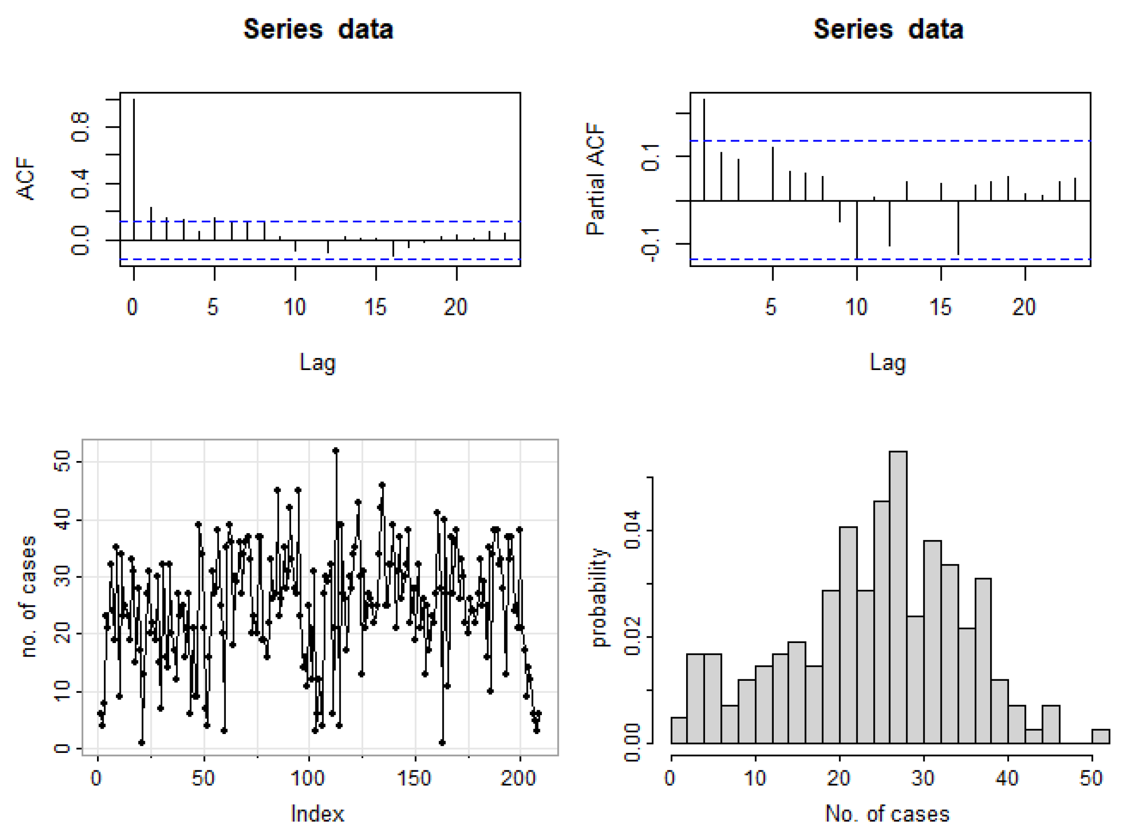
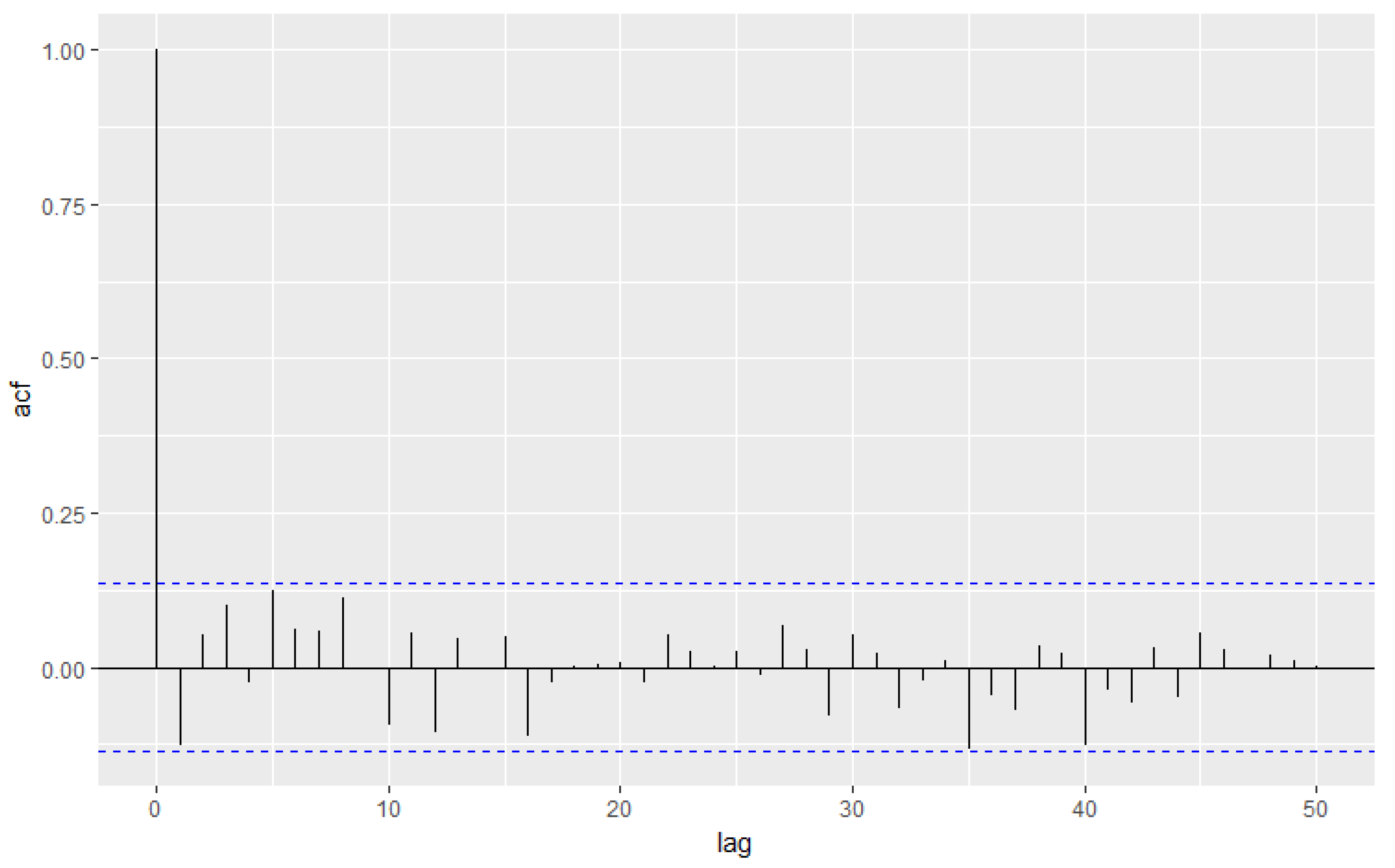
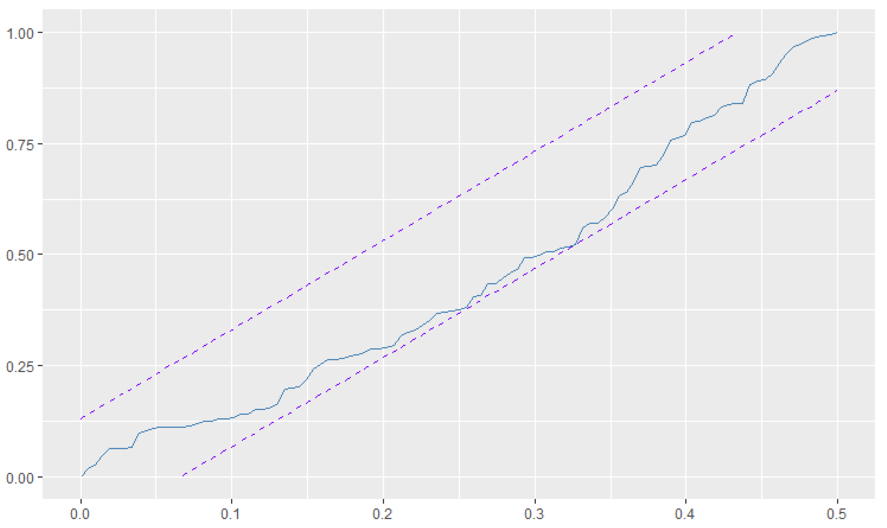
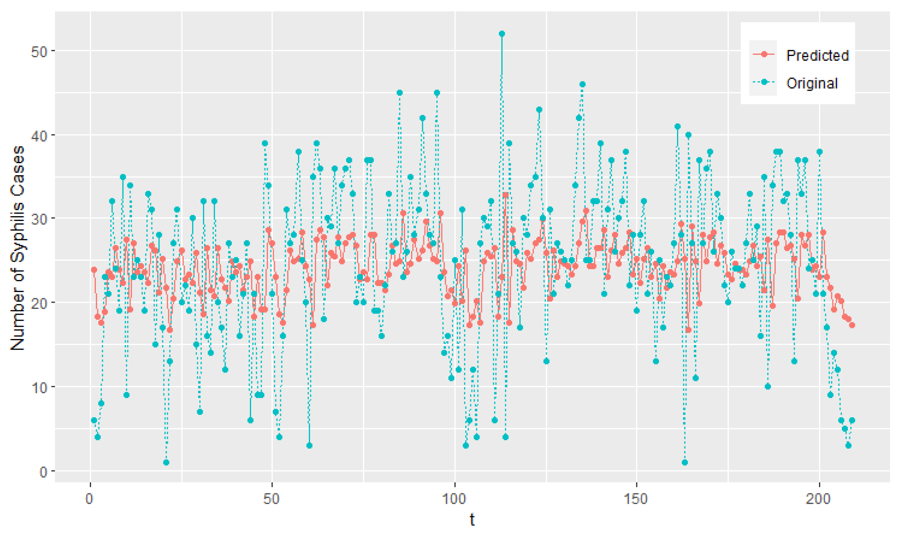
5.2. Weekly Number of Syphilis Cases Data

Weekly number of syphilis cases data, available in the tsinteger package of the R software, were fitted to the INAR(1)PNXL process. The effectiveness of this process was evaluated against the INAR(1)P process [30], the INAR(1)G process [12], the INAR(1)ZIP process [31], and the INAR(1)PWE process [17]. The dataset has a mean of 24.632 and a variance of 105.676, which shows significant over-dispersion.
The Pearson residuals are employed in residual analysis to assess statistical precision of the fitted INAR(1)PNXL process. These were calculated using
r t = x t E x t | X t 1 = x t 1 V x t | X t 1 = x t 1 1 2 ,
where E x t | X t 1 = x t 1 and V x t | X t 1 = x t 1 are given in (4) and (5), respectively. When the fitted INAR(1) process was statistically valid, the Pearson residuals had to be uncorrelated and should have zero mean and unit variance. The Pearson residuals are evaluated for correlation by generating a plot of their ACF. The randomness of the INAR(1)PNXL process can be examined by plotting cumulative periodograms (cpgrams) of the Pearson residuals for the series under consideration.
The ACF plot, partial ACF (PACF) plot, histogram, and time series plot of the data are shown in Figure 2. Only the first lag is noticeable in the PACF plot. So, the INAR(1) process could be a viable process for these data. The results of the INAR(1) process fitted to the data are shown in Table 5, together with parameter estimates, SEs, AICs, BICs, theoretical means, variances, and DIs.
The INAR(1)PNXL process offers a better fit than other INAR(1) processes as it gives the lowest AIC and lowest BIC values. The accuracy of the fitted INAR(1)PNXL process was assessed using standardized Pearson residuals. Figure 3 presents the ACF for the Pearson residuals, revealing the absence of autocorrelation. To confirm this, a Ljung–Box test was conducted with 10 degrees of freedom, resulting in a p-value of 0.1119, which is greater than 0.05. This test unequivocally establishes the lack of correlation among the residuals, providing strong evidence for the accuracy and excellent fit of the INAR(1)PNXL process to the weekly number of syphilis cases dataset. Figure 4 shows that the INAR(1)PNXL process is random for the weekly number of syphilis cases data.
The INAR(1)PNXL model for the weekly number of syphilis cases data is given by
X t = 0.316 X t 1 + ϵ t ,
where ϵ t P N X L ( 0.092 ) . The predicted values for the weekly number of syphilis cases data obtained by the INAR(1)PNXL process are the following:
X 1 ^ = E X t θ ^ c m l = 23.943 , X t ^ = E X t | X t 1 θ ^ c m l = 0.316 X t 1 + 16.388 , t = 2 , 3 , , n .
Figure 5 plots the predicted versus the original values of the weekly number of syphilis cases.

6. Conclusions

The PNXL distribution, a one-parameter discrete compound distribution capable of modeling data with over-dispersion, was proposed in this paper. Various probabilistic and statistical aspects, almost all of which have closed forms, show how adaptable and straightforward the one-parameter distribution is. Various methods were used to estimate its parameter. Simulation studies showed that ML and MM methods performed equally well in finite samples. Also, a new INAR(1)PNXL model was proposed. The better performance of the PNXL distribution or the INAR(1)PNXL model was illustrated using two real datasets, which was superior to several existing two-parameter models.

Author Contributions

Methodology, M.R.I., S.A., R.M. and S.N. All authors have read and agreed to the published version of the manuscript.

Funding

This research received no external funding.

Data Availability Statement

Data can be obtained from the corresponding author.

Acknowledgments

The authors would like to thank the editor and the three referees for careful reading and comments which greatly improved the paper.

Conflicts of Interest

The authors declare no conflict of interest.

References

  1. Bliss, C.I.; Fisher, R.A. Fitting the negative binomial distribution to biological data. Biometrics 1953, 9, 176–200. [Google Scholar] [CrossRef]
  2. Bereta, E.M.; Louzanda, F.; Franco, M.A. The Poisson-Weibull distribution. Adv. Appl. Stat. 2011, 22, 107–118. [Google Scholar]
  3. Sellers, K.F.; Borle, S.; Shmueli, G. The COM-Poisson model for count data: A survey of methods and applications. Appl. Stoch. Model. Bus. Ind. 2012, 28, 104–116. [Google Scholar] [CrossRef]
  4. Abd El-Monsef, M.; Sohsah, N. Poisson–transmuted Lindley distribution. J. Adv. Math. 2016, 11, 5631–5638. [Google Scholar] [CrossRef]
  5. Bhati, D.; Kumawat, P.; Gómez-Déniz, E. A new count model generated from mixed Poisson transmuted exponential family with an application to health care data. Commun. Stat. Theory Methods 2017, 46, 11060–11076. [Google Scholar] [CrossRef]
  6. Grine, R.; Zeghdoudi, H. On Poisson quasi-Lindley distribution and its applications. J. Mod. Appl. Stat. Methods 2017, 16, 21. [Google Scholar] [CrossRef]
  7. Altun, E. A new one-parameter discrete distribution with associated regression and integer-valued autoregressive models. Math. Slovaca 2020, 70, 979–994. [Google Scholar] [CrossRef]
  8. Altun, E.; Cordeiro, G.M.; Ristić, M.M. An one-parameter compounding discrete distribution. J. Appl. Stat. 2022, 49, 1935–1956. [Google Scholar] [CrossRef]
  9. Maya, R.; Chesneau, C.; Krishna, A.; Irshad, M.R. Poisson Extended Exponential Distribution with Associated INAR(1) Process and Applications. Stats 2022, 5, 755–772. [Google Scholar] [CrossRef]
  10. Irshad, M.; D’cruz, V.; Maya, R.; Mamode Khan, N. Inferential properties with a novel two parameter Poisson generalized Lindley distribution with regression and application to INAR(1) process. J. Biopharm. Stat. 2023, 33, 335–356. [Google Scholar] [CrossRef]
  11. Al-Osh, M.A.; Alzaid, A.A. First-order integer-valued autoregressive (INAR(1)) process. J. Time Ser. Anal. 1987, 8, 261–275. [Google Scholar] [CrossRef]
  12. Aghababaei Jazi, M.; Jones, G.; Lai, C.D. Integer valued AR(1) with geometric innovations. J. Iran. Stat. Soc. 2012, 11, 173–190. [Google Scholar]
  13. Eliwa, M.S.; Altun, E.; El-Dawoody, M.; El-Morshedy, M. A new three-parameter discrete distribution with associated INAR(1) process and applications. IEEE Access 2020, 8, 91150–91162. [Google Scholar] [CrossRef]
  14. Huang, J.; Zhu, F. A new first-order integer-valued autoregressive model with Bell innovations. Entropy 2021, 23, 713. [Google Scholar] [CrossRef] [PubMed]
  15. Altun, E.; El-Morshedy, M.; Eliwa, M. A study on discrete Bilal distribution with properties and applications on integer valued autoregressive process. REVSTAT-Stat. J. 2022, 20, 501–528. [Google Scholar]
  16. Lívio, T.; Khan, N.M.; Bourguignon, M.; Bakouch, H.S. An INAR(1) model with Poisson–Lindley innovations. Econ. Bull. 2018, 38, 1505–1513. [Google Scholar]
  17. Altun, E. A new generalization of geometric distribution with properties and applications. Commun. Stat. Simul. Comput. 2020, 49, 793–807. [Google Scholar] [CrossRef]
  18. Altun, E.; Bhati, D.; Khan, N.M. A new approach to model the counts of earthquakes: INARPQX(1) process. SN Appl. Sci. 2021, 3, 1–17. [Google Scholar] [CrossRef]
  19. Irshad, M.R.; Chesneau, C.; D’cruz, V.; Maya, R. Discrete pseudo Lindley distribution: Properties, estimation and application on INAR(1) process. Math. Comput. Appl. 2021, 26, 76. [Google Scholar] [CrossRef]
  20. Altun, E.; Khan, N.M. Modelling with the novel INAR(1)-PTE process. Methodol. Comput. Appl. Probab. 2022, 24, 1–17. [Google Scholar] [CrossRef]
  21. Nawel, K.; Gemeay, A.M.; Zeghdoudi, H.; Karakaya, K.; Alshangiti, A.M.; Bakr, M.; Balogun, O.S.; Muse, A.H.; Hussam, E. Modelling Voltage Real Dataset by a New Version of Lindley Distribution. IEEE Access 2023, 11, 67220–67229. [Google Scholar]
  22. Beghriche, A.; Zeghdoudi, H.; Raman, V.; Chouia, S. New polynomial exponential distribution: Properties and applications. Stat. Transit. New Ser. 2022, 23, 95–112. [Google Scholar] [CrossRef]
  23. Weiß, C.H. An Introduction to Discrete-Valued Time Series; John Wiley & Sons: Hoboken, NJ, USA, 2018. [Google Scholar]
  24. Bodhisuwan, W.; Sangpoom, S. The discrete weighted Lindley distribution. In Proceedings of the 2016 12th International Conference on Mathematics, Statistics, and Their Applications, ICMSA, Banda Aceh, Indonesia, 4–6 October 2016. [Google Scholar]
  25. Krishna, H.; Pundir, P.S. Discrete Burr and discrete Pareto distributions. Stat. Methodol. 2009, 6, 177–188. [Google Scholar] [CrossRef]
  26. Jazi, M.A.; Lai, C.D.; Alamatsaz, M.H. A discrete inverse Weibull distribution and estimation of its parameters. Stat. Methodol. 2010, 7, 121–132. [Google Scholar] [CrossRef]
  27. Chakraborty, S.; Chakravarty, D. A Discrete Gumbel Distribution. arXiv 2014, arXiv:1410.7568. [Google Scholar]
  28. Hussain, T.; Ahmad, M. Discrete inverse Rayleigh distribution. Pak. J. Stat. 2014, 30, 203–222. [Google Scholar]
  29. Para, B.A.; Jan, T.R. Discrete version of log-logistic distribution and its applications in genetics. Int. J. Mod. Math. Sci. 2016, 14, 407–422. [Google Scholar]
  30. McKenzie, E. Some simple models for discrete variate time series 1. J. Am. Water Resour. Assoc. 1985, 21, 645–650. [Google Scholar] [CrossRef]
  31. Jazi, M.A.; Jones, G.; Lai, C.D. First-order integer valued AR processes with zero inflated Poisson innovations. J. Time Ser. Anal. 2012, 33, 954–963. [Google Scholar] [CrossRef]
Figure 1. Pmf of the PNXL distribution for θ = 0.25 .
Mathematics 12 00081 g001
Figure 2. ACF plot, PACF plot, time series plot, and histogram of weekly number of syphilis cases data.
Mathematics 12 00081 g002
Figure 3. The ACF plot of the Pearson residuals.
Mathematics 12 00081 g003
Figure 4. The cpgrams of the Pearson residuals of the weekly number of syphilis cases data.
Mathematics 12 00081 g004
Figure 5. The predicted versus the original values of the weekly number of syphilis cases data.
Mathematics 12 00081 g005
Table 1. Simulation results for the PNXL distribution.
nMLEMMELSEWLSE
BiasMSEBiasMSEBiasMSEBiasMSE
θ = 0.5
500.0650.0040.0670.0040.1410.0200.1580.025
1000.0550.0030.0520.0030.1270.0160.1610.026
2000.0440.0020.0440.0020.1260.0160.1650.027
2500.0080.0000.0050.0000.0850.0070.1450.021
5000.0040.0000.0020.0000.1030.0110.0520.020
θ = 0.3
500.0340.0010.0370.0010.0870.0080.0740.006
1000.0130.0000.0150.0000.0580.0030.0590.004
2000.0080.0000.0080.0000.0500.0030.0600.004
2500.0070.0000.0080.0000.0320.0010.0450.002
5000.0010.0000.0010.0000.0030.0010.0350.001
θ = 1.2
500.1070.0110.1080.0120.5110.2610.6350.403
1000.0480.0020.0460.0020.4850.2350.6110.373
2000.0460.0020.0460.0020.4850.2350.6420.412
2500.0070.0050.0060.0000.4710.2220.6450.416
5000.0040.0000.0060.0010.4830.2340.5600.314
θ = 1.5
500.0550.0030.0520.0030.6840.4680.8970.804
1000.0300.0010.0290.0010.6770.4580.8680.754
2000.0250.0010.0260.0010.6890.4750.8800.775
2500.0210.0000.0250.0010.6990.4890.8640.747
5000.0200.0000.0210.0020.6660.4440.8890.790
Table 2. Simulation results for the INAR(1)PNXL process.
Parametern α = 0.4 and θ = 0.8
CMLCLSYW
BiasMSEBiasMSEBiasMSE
α 500.0630.0060.1090.0190.1100.020
1000.0440.0030.0800.0100.0810.010
2000.0320.0020.0540.0050.0530.005
2500.0290.0010.0490.0040.0490.004
5000.0190.0010.0350.0020.0350.002
θ 500.1300.0290.1640.0440.1620.043
1000.0940.0150.1220.0250.1220.025
2000.0630.0070.0840.0120.0830.012
2500.0580.0050.0780.0100.0780.010
5000.0410.0030.0560.0050.0560.005
α = 0.8 and θ = 3
α 500.0410.0030.0980.0170.1050.019
1000.0280.0010.0610.0070.0650.008
2000.0220.0010.0470.0040.0490.004
2500.0180.0010.0360.0020.0360.002
5000.0120.0000.0250.0010.0250.001
θ 500.7450.9781.0241.7221.0081.691
1000.5120.4550.7640.9230.7610.925
2000.3910.2410.6480.6520.6550.665
2500.2990.1480.4990.4050.5000.407
5000.2120.0700.3770.2230.3770.222
Table 3. Corn borer data: MLEs, SEs, and CIs.
StatisticPNXLDIWDGDLLDBDIRDBLDPCMP
M L E θ 1.0120.3453.1061.9432.3570.3200.6570.3290.672
S E θ 0.1110.0430.3670.1880.3660.0420.0190.0340.090
95% CIlower0.7940.2612.3881.5751.6410.2370.6200.2630.496
upper1.2300.4293.8252.3113.0730.4020.6930.3950.847
M L E β -1.5410.4071.4010.519---0.107
S E β -0.1560.0290.1210.051---0.116
95% CIlower-1.2350.3491.1630.419---0.121
upper-1.8470.4641.6380.619---0.334
Table 4. Corn borer data: log L , χ 2 -value, p-value, AIC, and BIC for the competitive models.
XOfPNXLDIWDGDLLDBDIRDBLDPCMP
04345.35541.37028.55341.03243.83638.35232.73464.44744.995
13530.08841.85037.86138.93839.60151.87439.58620.14930.221
21718.70515.42025.58517.77515.62215.48924.2779.68618.855
31111.1617.17012.8528.4327.2066.02812.5085.64711.266
456.4743.9405.7004.4853.9102.9055.9703.6816.529
543.6782.4202.4022.6302.3761.6102.7382.5803.695
612.0571.6100.9911.6631.5630.9811.2271.9042.051
721.1361.1300.4051.1151.0890.6410.5421.4611.120
821.3475.0905.6513.9304.7982.1200.42010.4461.271
Total120120120120120120120120120120
log L ---------
200.432204.810231.191202.630204.293208.440204.675220.618200.415
AIC402.863413.621430.382409.261412.587418.881411.351443.236404.830
BIC405.651419.195435.957414.836418.162421.668414.138446.024410.405
χ 2 1.1155.5117.6151.3112.67414.2956.99630.5181.063
df332223332
p-value0.7740.1380.0220.5190.2630.0030.0720.0000.588
Table 5. Estimates and model adequacy statistics of the fitted models for the number of syphilis cases data.
ModelParametersEstimateS.E.AICBIC μ σ 2 DI
INAR(1)PNXL α 0.3160.0341660.8691667.55423.943255.91710.689
θ 0.0920.007
INAR(1)P α 0.1480.0262016.5342023.22425.34925.3491.000
λ 21.0630.709
INAR(1)G α 0.3470.0321686.4281693.11223.895252.43110.564
λ 0.0580.005
INAR(1)PWE α 0.0580.1591688.4281698.45524.990369.21114.774
λ 0.0602.883
β 0.3470.032
INAR(1)ZIP α 20.5520.5951732.2961742.32325.33258.5432.307
λ 0.1130.024
β 0.2620.024
Disclaimer/Publisher’s Note: The statements, opinions and data contained in all publications are solely those of the individual author(s) and contributor(s) and not of MDPI and/or the editor(s). MDPI and/or the editor(s) disclaim responsibility for any injury to people or property resulting from any ideas, methods, instructions or products referred to in the content.

