


Application of Artificial Intelligence Methods for Predicting the Compressive Strength of Green Concretes with Rice Husk Ash

 ,
,  ,
, 
 and
and
Abstract
:1. Introduction
2. Materials and Methods
2.1. Multiple Linear Regression Model
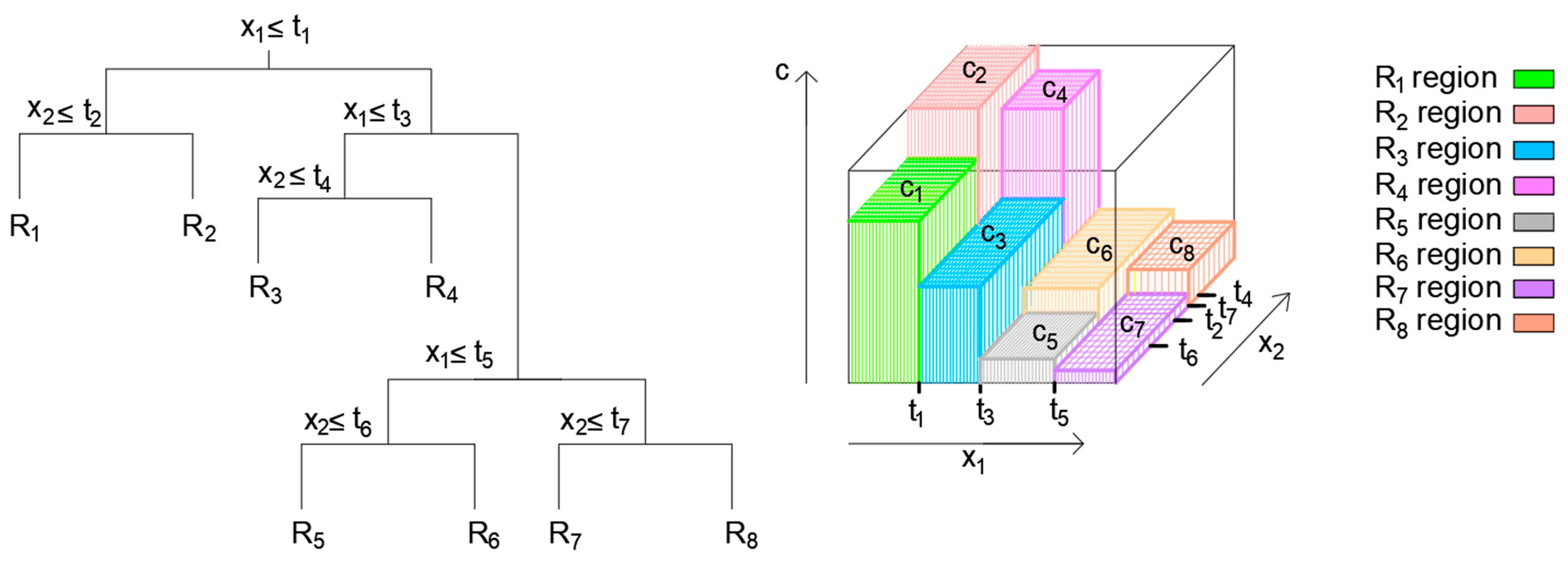
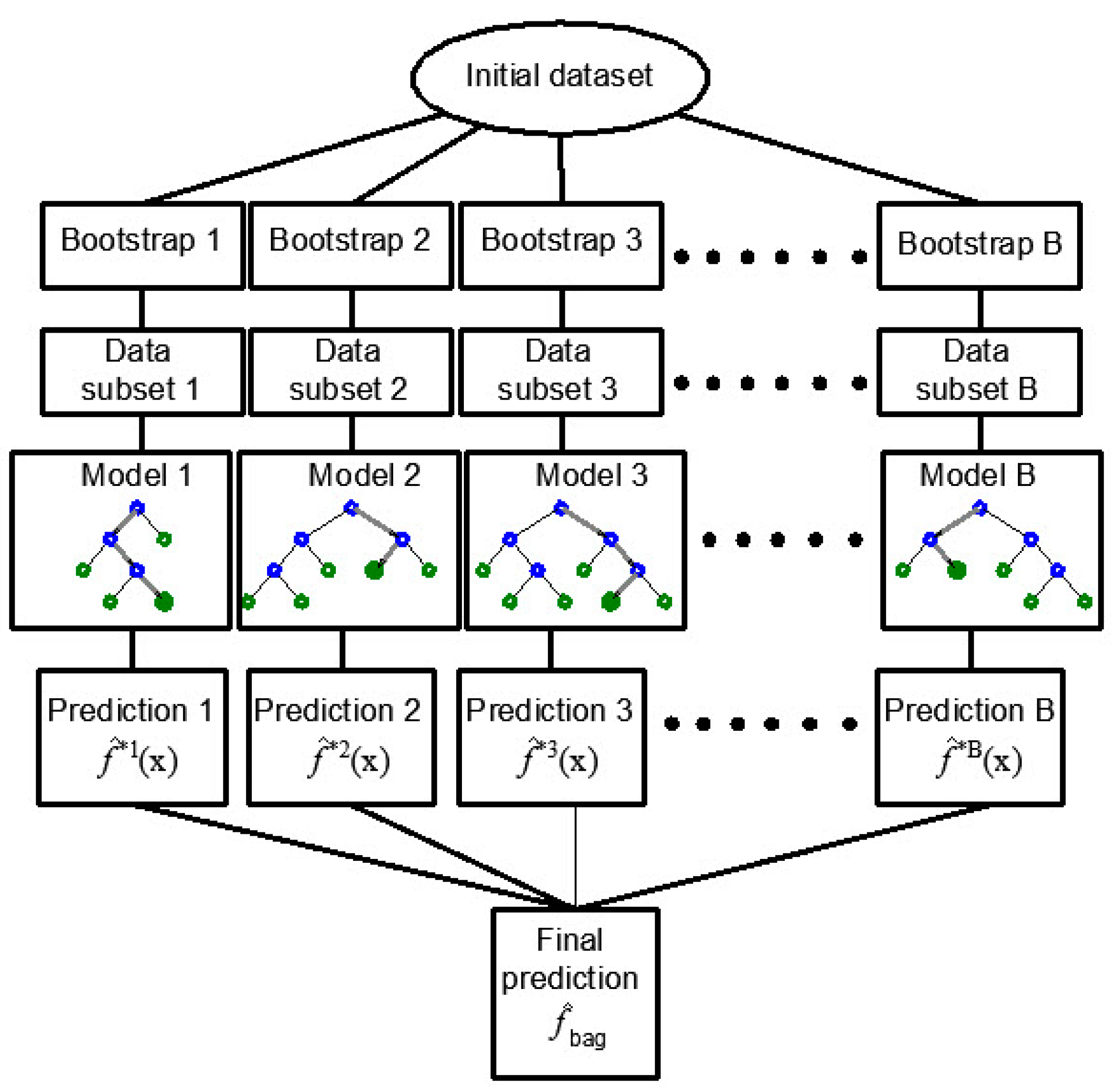
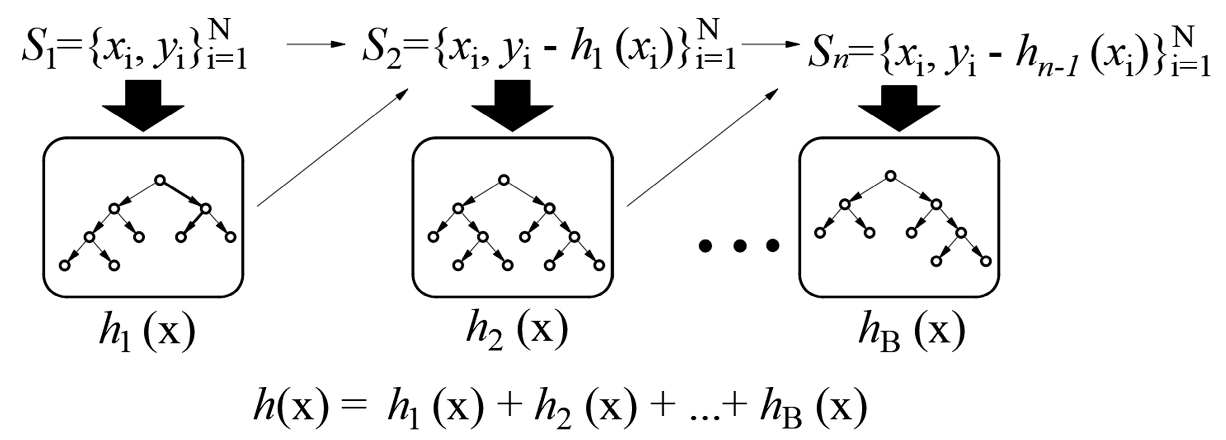
2.2. Regression Trees Ensembles: Bagging, Random Forest, and Boosted Trees
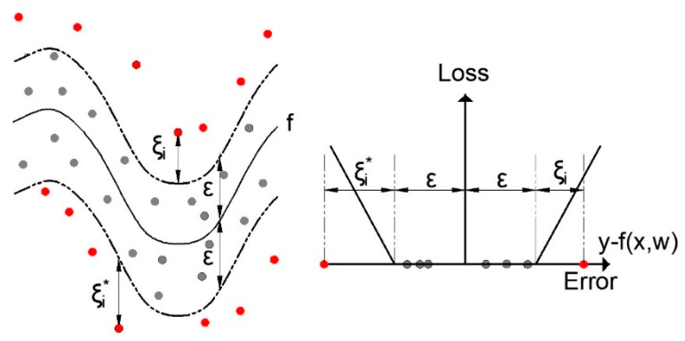
2.3. Support Vector Machine for Regression (SVR)
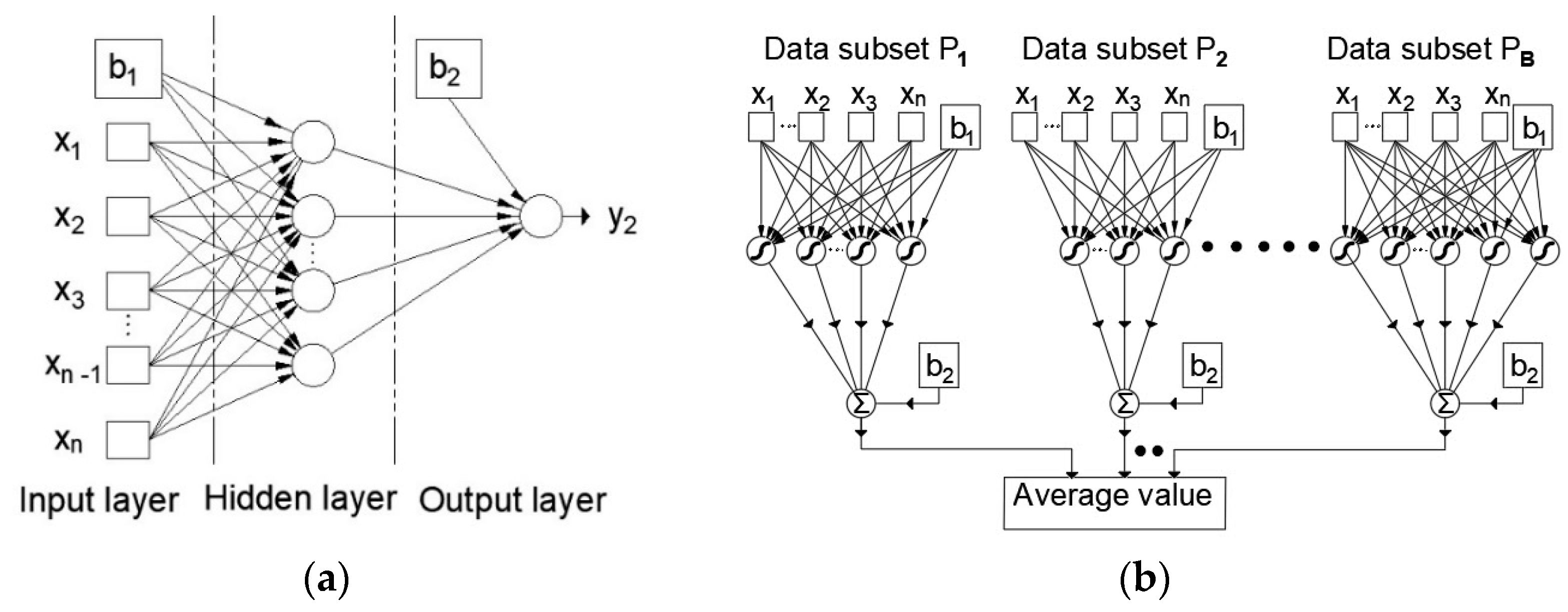
2.4. Artificial Neural Network and Artificial Neural Networks Ensemble
2.5. Gaussian Process for Regression (GPR)
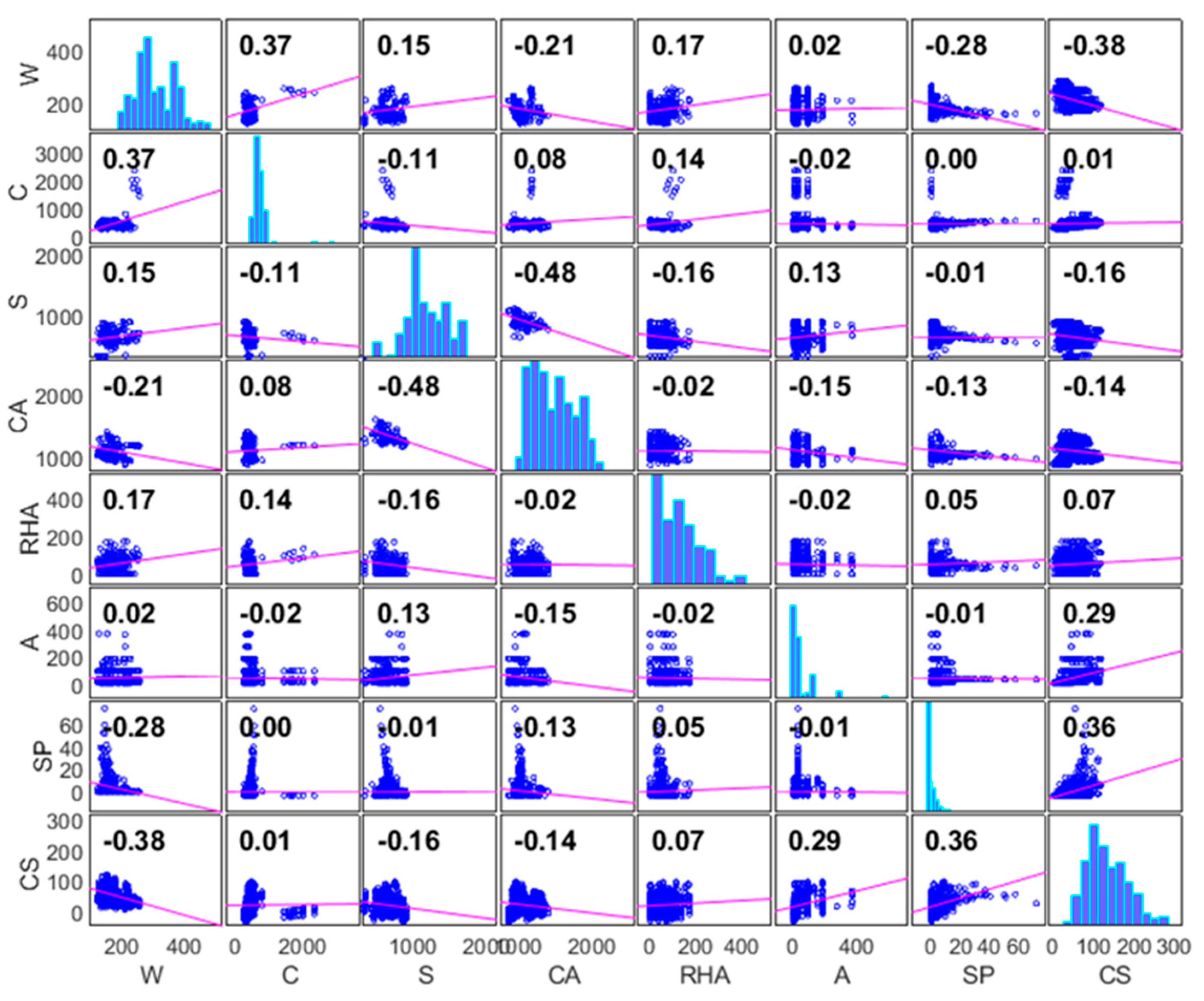
3. Dataset
4. Results and Discussion
- Multiple linear regression,
- Bagging method (TreeBagger—TB),
- Random Forests (RF) method,
- Boosted Trees (BT) method,
- Support vector regression,
- Neural networks (standalone and ensamble models),
- Gaussian proces regression (GPR).
- Number of generated trees (B). Throughout this analysis, the maximum number of generated trees was constrained to 500.
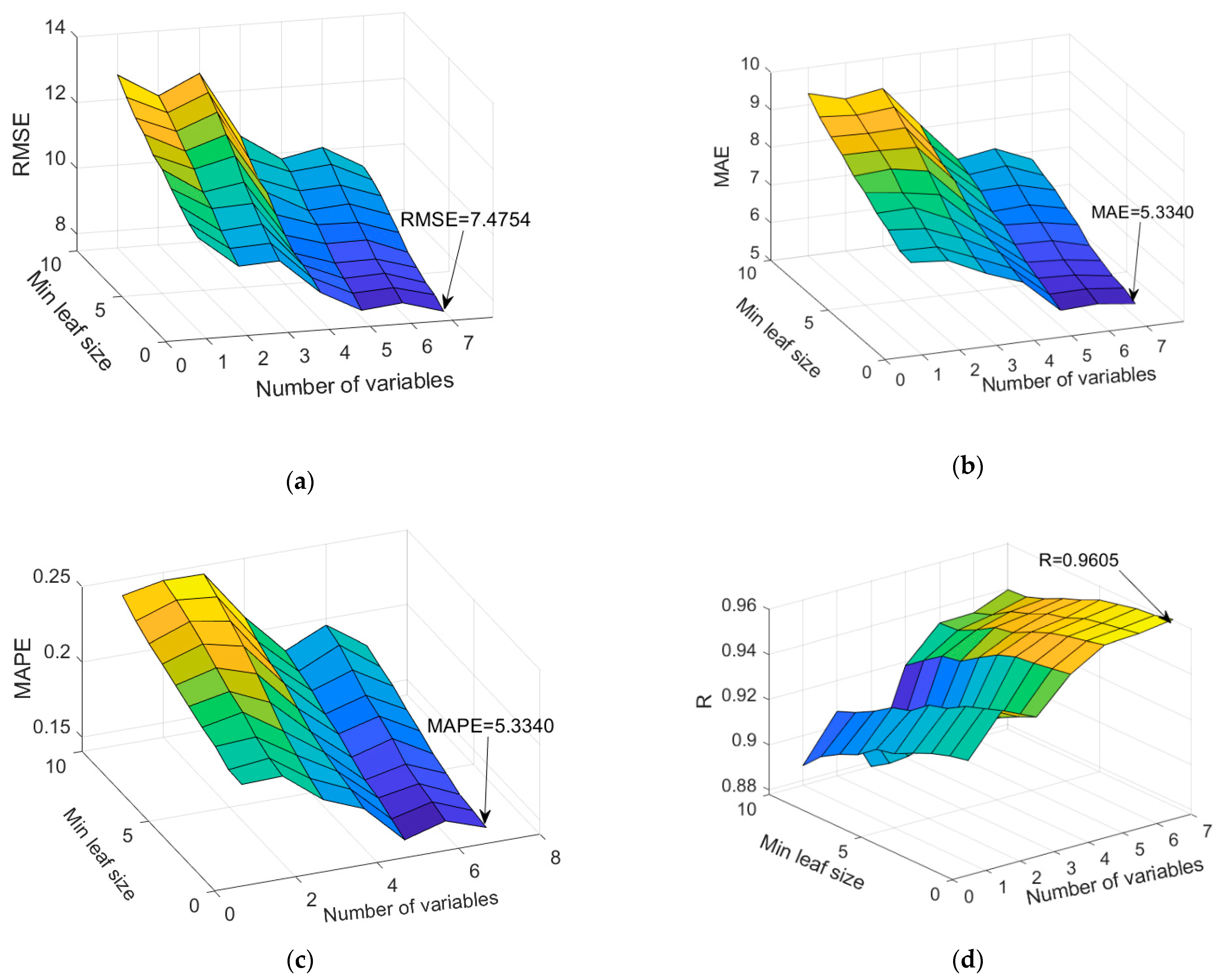
- The number of variables utilized for splitting within the tree. TB and RF models operate on a similar mechanism, with the key distinction being that the TB model employs all variables as potential tree split points, while the RF model uses only a specific subset of the entire variable set. Following the recommendation in L. Bryman’s paper on Random Forests [39], it is advised that the subset m of variables for splitting should be p/3 of the total number of variables or predictors p. In this study, values of m from 1 to 7 (Figure 7) were examined.
- The minimum number of data or samples assigned to a leaf (min leaf size) within a tree. Consideration was given to values ranging from 1 to 10 samples per tree leaf.
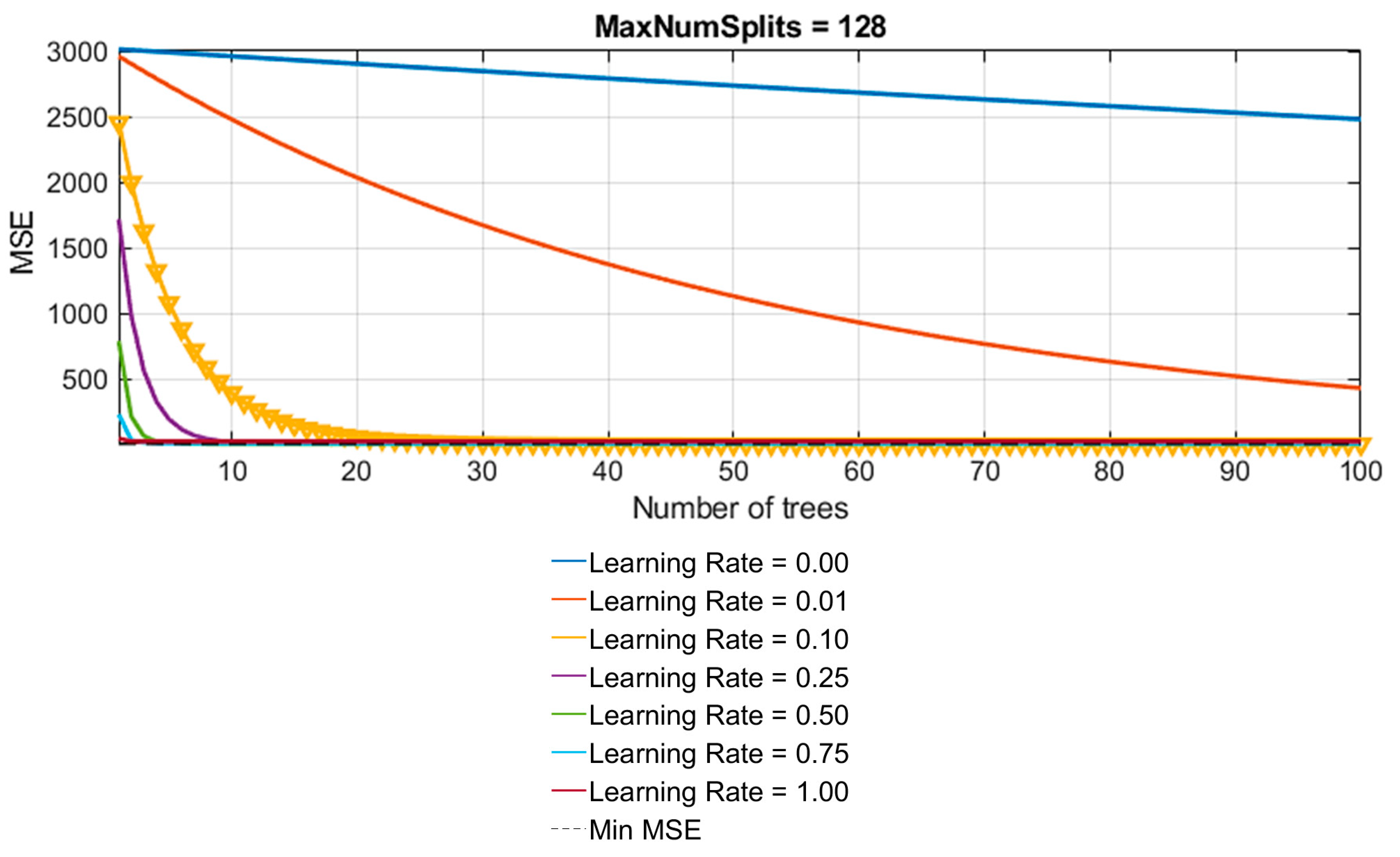
- Number of generated trees (B): To prevent overtraining, the maximum limit of base models within the ensemble was set to 100.
- Learning rate (λ): This parameter, determining the model’s training speed, was investigated across various values, including 0.001, 0.01, 0.1, 0.25, 0.5, 0.75, and 1.0.
- Linear Kernel: C = 38.27, ε = 0.1012
- RBF Kernel: C = 94.26, ε = 0.0164, γ = 3.3364
- Sigmoid Kernel: C = 121.10, ε = 0.0947, γ = 0.0085.
- squaring the difference between the target and forecast values,
- calculating the average, and
- subsequently determining the square root of this value.
5. Conclusions
Author Contributions
Funding
Data Availability Statement
Acknowledgments
Conflicts of Interest
References
- Thomas, B.S. Green concrete partially comprised of rice husk ash as a supplementary cementitious material—A comprehensive review. Renew. Sustain. Energy Rev. 2018, 82, 3913–3923. [Google Scholar] [CrossRef]
- Sheheryar, M.; Rehan, R.; Nehdi, M.L. Estimating CO2 emission savings from ultrahigh performance concrete: A system dynamics approach. Materials 2021, 14, 995. [Google Scholar] [CrossRef]
- Suhendro, B. Toward green concrete for better sustainable environment. Procedia Eng. 2014, 95, 305–320. [Google Scholar] [CrossRef]
- United States Department of Agriculture. Grain: World Markets and Trade Report. 2023. Available online: https://fas.usda.gov/data/grain-world-markets-and-trade (accessed on 14 December 2023).
- Data Bridge Market Research Market Analysis Study. 2022. Available online: https://www.databridgemarketresearch.com/reports/global-rice-husk-ash-market (accessed on 1 June 2023).
- Aprianti, E. A huge number of artificial waste material can be supplementary cementitious material (SCM) for concrete production—A review part, II. J. Clean. Prod. 2017, 142, 4178–4194. [Google Scholar] [CrossRef]
- Boindala, S.P.; Ramagiri, K.K.; Alex, A.; Kar, A. Step-Wise Multiple Linear Regression Model Development for Shrinkage Strain Prediction of Alkali Activated Binder Concrete. In Proceedings of SECON’19; Lecture Notes in Civil Engineering; Dasgupta, K., Sajith, A., Unni Kartha, G., Joseph, A., Kavitha, P., Praseeda, K., Eds.; Springer: Cham, Germany, 2020; Volume 46. [Google Scholar] [CrossRef]
- Ramagiri, K.K.; Boindala, S.P.; Zaid, M.; Kar, A. Random Forest-Based Algorithms for Prediction of Compressive Strength of Ambient-Cured AAB Concrete—A Comparison Study. In Proceedings of SECON’21; Lecture Notes in Civil Engineering; Marano, G.C., Ray Chaudhuri, S., Unni Kartha, G., Kavitha, P.E., Prasad, R., Achison, R.J., Eds.; Springer: Cham, Germany, 2020; Volume 171. [Google Scholar] [CrossRef]
- Zhang, M.H.; Lastra, R.; Malhotra, V.M. Rice-husk ash paste and concrete: Some aspects of hydration and the microstructure of the interfacial zone between the aggregate and paste. Cem. Concr. Res. 1996, 26, 963–977. [Google Scholar] [CrossRef]
- Sata, V.; Jaturapitakkul, C.; Kiattikomol, K. Influence of pozzolan from various by-product materials on mechanical properties of high-strength concrete. Constr. Build. Mater. 2007, 21, 1589–1598. [Google Scholar] [CrossRef]
- Antiohos, S.; Tapali, J.; Zervaki, M.; Sousa-Coutinho, J.; Tsimas, S.; Papadakis, V. Low embodied energy cement containing untreated RHA: A strength development and durability study. Constr. Build. Mater. 2013, 49, 455–463. [Google Scholar] [CrossRef]
- Prasittisopin, L.; Trejo, D. Hydration and phase formation of blended cementitious systems incorporating chemically transformed rice husk ash. Cem. Concr. Compos. 2015, 59, 100–106. [Google Scholar] [CrossRef]
- Mehta, P.; Pirtz, D. Use of rice hull ash to reduce temperature in high-strength mass concrete. J. Proc. 1978, 75, 60–63. [Google Scholar] [CrossRef]
- Kishore, R.; Bhikshma, V.; Prakash, P.J. Study on strength characteristics of high strength rice husk ash concrete. Procedia Eng. 2011, 14, 2666–2672. [Google Scholar] [CrossRef]
- Ganesan, K.; Rajagopal, K.; Thangavel, K. Rice husk ash blended cement: Assessment of optimal level of replacement for strength and permeability properties of concrete. Constr. Build. Mater. 2008, 22, 1675–1683. [Google Scholar] [CrossRef]
- Giaccio, G.; de Sensale, G.R.; Zerbino, R. Failure mechanism of normal and high-strength concrete with rice-husk ash. Cem. Concr. Compos. 2007, 29, 566–574. [Google Scholar] [CrossRef]
- de Sensale, G.R. Strength development of concrete with rice-husk ash. Cem. Concr. Compos. 2006, 28, 158–160. [Google Scholar] [CrossRef]
- Sam, J. Compressive strength of concrete using fly ash and rice husk ash: A review. Civ. Eng. J. 2020, 6, 1400–1410. [Google Scholar] [CrossRef]
- Hwang, C.L.; Chandra, S. The use of rice husk ash in concrete. In Waste Materials Used in Concrete Manufacturing; Chandra, S., Ed.; William Andrew Publishing: Norwich, NY, USA, 1996; pp. 184–234. ISBN 9780815513933. [Google Scholar] [CrossRef]
- Habeeb, G.A.; Mahmud, H.B. Study on properties of rice husk ash and its use as cement replacement material. Mater. Res. 2010, 13, 185–190. [Google Scholar] [CrossRef]
- Fapohunda, C.; Akinbile, B.; Shittu, A. Structure and properties of mortar and concrete with rice husk ash as partial replacement of ordinary Portland cement—A review. Int. J. Sustain. Built Env. 2017, 6, 675–692. [Google Scholar] [CrossRef]
- Nehdi, M.; Duquette, J.; Damatty, E.A. Performance of rice husk ash produced using a new technology as a mineral admixture in concrete. Cem. Concr. Res. 2003, 33, 1203–1210. [Google Scholar] [CrossRef]
- Shatat, M.R. Hydration behavior and mechanical properties of blended cement containing various amounts of rice husk ash in presence of metakaolin. Arab. J. Chem. 2016, 9, S1869–S1874. [Google Scholar] [CrossRef]
- Ahmed, A.E.; Adam, F. Indium incorporated silica from rice husk and its catalytic activity. Microporous Mesoporous Mater. 2007, 103, 284–295. [Google Scholar] [CrossRef]
- Badorul, H.A.B.; Ramadhansyah, P.C.; Hamidi, A.A. Malaysian rice husk ash—Improving the durability and corrosion resistance of concrete: Pre-review. EACEF–Int. Conf. Civ. Eng. 2011, 1, 607–612. Available online: https://proceeding.eacef.com/ojs/index.php/EACEF/article/view/428 (accessed on 5 November 2023).
- Habeeb, G.A.; Fayyadh, M.M. The effect of RHA average particle size on the mechanical properties and drying shrinkage. Aust. J. Basic. Appl. Sci. 2009, 3, 1616–1622. Available online: https://www.ajbasweb.com/old/ajbas/2009/1616-1622.pdf (accessed on 4 November 2023).
- Anwar, M.; Miyagawa, T.; Gaweesh, M. Using rice husk ash as a cement replacement material in concrete. Waste Manag. Ser. 2000, 1, 671–684. [Google Scholar] [CrossRef]
- Nagrale, S.D.; Hemant, H.; Modak, P.R. Utilization of rice husk ash. Int. J. Eng. Res. Appl. 2012, 2, 1–5. Available online: https://www.ijera.com/papers/Vol2_issue4/A24001005.pdf (accessed on 5 November 2023).
- Chindaprasirt, P.; Kanchanda, P.; Sathonsaowaphak, A.; Cao, H.T. Sulfate resistance of blended cements containing fly ash and rice husk ash. Constr. Build. Mater. 2007, 21, 1356–1361. [Google Scholar] [CrossRef]
- Khan, K.; Ullah, M.F.; Shahzada, K.; Amin, M.N.; Bibi, T.; Wahab, N.; Aljaafari, A. Effective use of micro-silica extracted from rice husk ash for the production of high-performance and sustainable cement mortar. Constr. Build. Mater. 2020, 258, 119589. [Google Scholar] [CrossRef]
- Iqtidar, A.; Bahadur Khan, N.; Kashif-ur-Rehman, S.; Faisal Javed, M.; Aslam, F.; Alyousef, R.; Alabduljabbar, H.; Mosavi, A. Prediction of Compressive Strength of Rice Husk Ash Concrete through Different Machine Learning Processes. Crystals 2021, 11, 352. [Google Scholar] [CrossRef]
- Amin, M.N.; Iftikhar, B.; Khan, K.; Javed, M.F.; AbuArab, A.M.; Rehman, M.F. Prediction model for rice husk ash concrete using AI approach: Boosting and bagging algorithms. Structures 2023, 50, 745–757. [Google Scholar] [CrossRef]
- Amlashi, A.T.; Golafshani, E.M.; Ebrahimi, S.A.; Behnood, A. Estimation of the compressive strength of green concretes containing rice husk ash: A comparison of different machine learning approaches. Eur. J. Environ. Civ. Eng. 2023, 27, 961–983. [Google Scholar] [CrossRef]
- Bassi, A.; Manchanda, A.; Singh, R.; Patel, M. A comparative study of machine learning algorithms for the prediction of compressive strength of rice husk ash-based concrete. Nat. Hazards 2023, 118, 209–238. [Google Scholar] [CrossRef]
- Li, C.; Mei, X.; Dias, D.; Cui, Z.; Zhou, J. Compressive Strength Prediction of Rice Husk Ash Concrete Using a Hybrid Artificial Neural Network Model. Materials 2023, 16, 3135. [Google Scholar] [CrossRef]
- Amin, M.N.; Ahmad, W.; Khan, K.; Deifalla, A.F. Optimizing compressive strength prediction models for rice husk ash concrete with evolutionary machine intelligence techniques. Case Stud. Constr. Mater. 2023, 18, e02102. [Google Scholar] [CrossRef]
- Kovačević, M.; Lozančić, S.; Nyarko, E.K.; Hadzima-Nyarko, M. Modeling of Compressive Strength of Self-Compacting Rubberized Concrete Using Machine Learning. Materials 2021, 14, 4346. [Google Scholar] [CrossRef] [PubMed]
- Hastie, T.; Tibsirani, R.; Friedman, J. The Elements of Statistical Learning; Springer: Berlin/Heidelberg, Germany, 2009. [Google Scholar]
- Breiman, L.; Friedman, H.; Olsen, R.; Stone, C.J. Classification and Regression Trees; Chapman and Hall/CRC: Wadsworth, OH, USA, 1984. [Google Scholar]
- Breiman, L. Bagging Predictors. Mach. Learn. 1996, 24, 123–140. [Google Scholar] [CrossRef]
- Breiman, L. Random Forests. Mach. Learn. 2001, 45, 5–32. [Google Scholar] [CrossRef]
- Kovačević, M.; Ivanišević, N.; Petronijević, P.; Despotović, V. Construction cost estimation of reinforced and prestressed concrete bridges using machine learning. Građevinar 2021, 73, 727. [Google Scholar] [CrossRef]
- Friedman, J.H. Greedy function approximation: A gradient boosting machine. Ann. Stat. 2001, 29, 1189–1232. [Google Scholar] [CrossRef]
- Elith, J.; Leathwick, J.R.; Hastie, T. A working guide to boosted regression trees. J. Anim. Ecol. 2008, 77, 802–813. [Google Scholar] [CrossRef]
- Friedman, J.H.; Meulman, J.J. Multiple additive regression trees with application in epidemiology. Stat. Med. 2003, 22, 1365–1381. [Google Scholar] [CrossRef]
- Vapnik, V. The Nature of Statistical Learning Theory; Springer: New York, NY, USA, 1995. [Google Scholar]
- Kecman, V. Learning and Soft Computing: Support Vector Machines, Neural Networks, and Fuzzy Logic Models; MIT Press: Cambridge, MA, USA, 2001. [Google Scholar]
- Smola, A.J.; Sholkopf, B. A tutorial on support vector regression. Stat. Comput. 2004, 14, 199–222. [Google Scholar] [CrossRef]
- Chang, C.C.; Lin, C.J. LIBSVM: A library for support vector machines. ACM Trans. Intell. Syst. Technol. 2011, 2, 1–27. [Google Scholar] [CrossRef]
- LIBSVM—A Library for Support Vector Machines. Available online: https://www.csie.ntu.edu.tw/~cjlin/libsvm/ (accessed on 21 February 2021).
- Rasmussen, C.E.; Williams, C.K. Gaussian Processes for Machine Learning; The MIT Press: Cambridge, MA, USA, 2006. [Google Scholar]
- Elwell, D.J.; Fu, G. Compression Testing of Concrete: Cylinders vs. Cubes; FHWA/NY/SR-95/119; New York State Department of Transportation: New York, NY, USA, 1995. [Google Scholar]
- Ikpong, A.A.; Okpala, D.C. Strength characteristics of medium workability ordinary Portland cement-rice husk ash concrete. Build. Environ. 1992, 27, 105–111. [Google Scholar] [CrossRef]
- Ismail, M.S.; Waliuddin, A.M. Effect of rice husk ash on high strength concrete. Constr. Build. Mater. 1996, 10, 521–526. [Google Scholar] [CrossRef]
- Zhang, M.H.; Malhotra, V.M. High-performance concrete incorporating rice husk ash as a supplementary cementing material. ACI Mater. J. 1996, 93, 629–636. [Google Scholar] [CrossRef]
- Feng, Q.G.; Lin, Q.Y.; Yu, Q.J.; Zhao, S.Y.; Yang, L.F.; Sugita, S. Concrete with highly active rice husk ash. J. Wuhan. Univ. Technol.-Mater. Sci. Ed. 2004, 79, 74–77. [Google Scholar] [CrossRef]
- Bui, D.D.; Hu, J.; Stroeven, P. Particle size effect on the strength of rice husk ash blended gap-graded Portland cement concrete. Cem. Concr. Compos. 2005, 27, 357–366. [Google Scholar] [CrossRef]
- Kartini, K.; Mahmud, H.; Hamidah, M. Strength properties of grade 30 rice husk ash. In Proceedings of the 31st Conference on Our World in Concrete & Structure, Singapore, 16–17 September 2006. [Google Scholar]
- Sakr, K. Effects of silica fume and rice husk ash on the properties of heavy weight concrete. J. Mater. Civ. Eng. 2006, 18, 367–376. [Google Scholar] [CrossRef]
- Saraswathy, V.; Song, H.W. Corrosion performance of rice husk ash blended concrete. Constr. Build. Mater. 2007, 2, 1779–1784. [Google Scholar] [CrossRef]
- Ganesan, K. Studies on the Performance of Rice Husk Ash and Bagasse Ash Blended Concretes for Durability Properties. Ph.D. Thesis, Anna University, Chennai, India, 2007. Available online: http://hdl.handle.net/10603/28700 (accessed on 5 November 2023).
- Mahmud, H.B.; Malik, M.F.A.; Kahar, R.A.; Zain, M.F.M.; Raman, S.N. Mechanical properties and durability of normal and water reduced high strength grade 60 concrete containing rice husk ash. J. Adv. Concr. Technol. 2009, 7, 21–30. [Google Scholar] [CrossRef]
- Mahmud, H.B.; Hamid, N.A.A.; Chin, K.Y. Production of high strength concrete incorporating an agricultural waste—Rice husk ash. In Proceedings of the 2nd International Conference on Chemical, Biological and Environmental Engineering, Cairo, Egypt, 2–4 November 2010; pp. 106–109. [Google Scholar] [CrossRef]
- Madandoust, R.; Ranjbar, M.M.; Moghadam, H.A.; Mousavi, S.Y. Mechanical properties and durability assessment of rice husk ash concrete. Biosyst. Eng. 2011, 110, 144–152. [Google Scholar] [CrossRef]
- Chao-Lung, H.; Anh-Tuan, B.L.; Chun-Tsun, C. Effect of rice husk ash on the strength and durability characteristics of concrete. Constr. Build. Mater. 2011, 25, 3768–3772. [Google Scholar] [CrossRef]
- Muthadhi, A. Studies on production of reactive rice husk ash and performance of RHA concrete. In Indian ETD Repository @ INFUBNET; Pondicherry University: Puducherry, India, 2012. [Google Scholar]
- Ramasamy, V. Compressive strength and durability properties of Rice Husk Ash concrete. KSCE J. Civ. Eng. 2012, 16, 93–102. [Google Scholar] [CrossRef]
- Islam, M.N.; Mohd Zain, M.F.; Jamil, M. Prediction of strength and slump of rice husk ash incorporated high-performance concrete. J. Civ. Eng. Manag. 2012, 18, 310–317. [Google Scholar] [CrossRef]
- Krishna, N.K.; Sandeep, S.; Mini, K.M. Study on concrete with partial replacement of cement by rice husk ash. IOP Conf. Ser. Mater. Sci. Eng. 2016, 149, 12109. [Google Scholar] [CrossRef]
- Singh, P. To study strength characteristics of concrete with rice husk ash. Indian. J. Sci. Technol. 2016, 9, 1–5. [Google Scholar] [CrossRef]
- Tandon, A.; Jawalkar, C.S. Improving strength of concrete through partial usage of rice husk ash. Int. Res. J. Eng. Technol. 2017, 4, 51–54. Available online: https://www.irjet.net/archives/V4/i7/IRJET-V4I709.pdf (accessed on 5 November 2023).
- Siddika, A.; Mamun, M.A.A.; Ali, M.H. Study on concrete with rice husk ash. Innov. Infrastruct. Solut. 2018, 3, 18. [Google Scholar] [CrossRef]
- He, Z.; Chang, J.; Liu, C.; Du, S.; Huang, M.A.N.; Chen, D. Compressive strengths of concrete containing rice husk ash without processing. Rev. Romana Mater./Rom. J. Mater. 2018, 48, 499–506. Available online: https://solacolu.chim.upb.ro/p499-506.pdf (accessed on 5 November 2023).
- Singh, R.R.; Singh, D. Effect of rice husk ash on compressive strength of concrete. Int. J. Struct. Civ. Eng. Res. 2019, 8, 223–226. [Google Scholar] [CrossRef]
- Kumar, P.C.; Rao, P.M. A study on reuse of Rice Husk Ash in Concrete. Pollut. Res. 2010, 29, 157–163. [Google Scholar] [CrossRef]
- Nisar, N.; Bhat, J.A. Experimental investigation of Rice Husk Ash on compressive strength, carbonation and corrosion resistance of reinforced concrete. Aust. J. Civ. Eng. 2021, 79, 155–163. [Google Scholar] [CrossRef]


| Num. of Data | Water (kg/m3) | Cement (kg/m3) | Fine Aggregate (FA) (kg/m3) | Coarse Aggregate (CA) (kg/m3) | RHA (kg/m3) | Age (Days) | SP (kg/m3) | CS (MPa) | Ref. |
|---|---|---|---|---|---|---|---|---|---|
| 48 | 215–255 | 300–2351 | 580–710 | 1160–1185 | 0–134 | 7–90 | 0 | 13.27–47.6 | [53] |
| 16 | 138–207 | 400–571 | 578–612 | 1027–1088 | 0–171 | 3–150 | 10–14.275 | 31.5–85 | [54] |
| 14 | 153–154 | 345–385 | 667–674 | 1086–1102 | 0–38 | 1–365 | 2.5–3.9 | 25.34–60.74 | [55] |
| 24 | 128 | 356–410 | 786 | 1044–1062 | 0–72 | 3–365 | 0 | 42–92 | [19] |
| 18 | 210 | 280–350 | 844–870 | 854–881 | 0–70 | 1–180 | 0 | 2.4–39.4 | [27] |
| 28 | 178–180 | 356–600 | 570–636 | 906–968 | 0–153 | 3–90 | 0.89–12.48 | 36.86–106.82 | [56] |
| 60 | 160–170 | 400–550 | 540–567 | 1261–1324 | 0–110 | 1–90 | 5–6.22 | 18.9–86.8 | [57] |
| 36 | 205–228 | 228–325 | 890–900 | 927–940 | 0–97 | 1–180 | 0–3.67 | 9.2–45.8 | [58] |
| 27 | 164–204 | 327–534 | 690–758 | 983–1050 | 0–85 | 7–91 | 0.462–4.33 | 29.22–77.96 | [17] |
| 20 | 150 | 375 | 770 | 1200 | 0–75 | 7–90 | 0–15 | 30–64 | [59] |
| 16 | 138–173 | 322–513 | 720–845 | 975–1045 | 0–34 | 28–90 | 0–10.26 | 37–82.1 | [16] |
| 20 | 150–153 | 392–560 | 735–764 | 943–981 | 0–168 | 7–180 | 1.5–9 | 103.06–118.82 | [10] |
| 21 | 201 | 266–380 | 570 | 1140 | 0–114 | 7–28 | 0 | 27.22–39.55 | [60] |
| 32 | 203 | 249–383 | 561 | 1148 | 0–134 | 7–90 | 0 | 27.22–45.98 | [61] |
| 32 | 131.97–202.99 | 249–383 | 575 | 1150 | 0–134 | 1–28 | 0 | 10.4–46.7 | [15] |
| 60 | 137–190 | 304–500 | 745–868 | 933–995 | 0–100 | 1–28 | 0–3.88 | 19–68.6 | [62] |
| 12 | 207 | 313–391 | 750 | 994 | 0–78 | 1– 180 | 0 | 19.1–48.1 | [26] |
| 16 | 157–173 | 492–518 | 484–510 | 983–1025 | 0–52 | 7–180 | 0 | 66.3–93.5 | [63] |
| 20 | 207 | 313–391 | 750 | 994 | 0–78 | 1–28 | 0 | 17.2–50.2 | [20] |
| 24 | 122.4–150.5 | 340–430 | 332–335 | 1012–1014 | 0–64.5 | 7–90 | 0 | 30.36–62.5 | [14] |
| 20 | 210 | 297–396 | 844 | 951 | 0–99 | 28–360 | 0 | 29.7–47.8 | [64] |
| 42 | 212–221 | 383–783 | 344–737 | 933 | 0–171 | 1–90 | 0.3–3.7 | 19.4–89.725 | [65] |
| 76 | 154–165 | 280–550 | 490–560 | 1200–1345 | 0–165 | 3–60 | 0.87–9.75 | 30.5–92 | [66] |
| 50 | 166 | 336–474 | 433.72–636 | 1108–1113 | 0–108 | 7–180 | 0–9.4 | 5.87–73 | [67] |
| 60 | 132.4–178.4 | 378.8–553.8 | 543.8–720.7 | 951.6–1048.3 | 25–71.7 | 28 | 5.3–93.0 | 51.5–111.8 | [68] |
| 5 | 192 | 278.7–348.4 | 573 | 1189.5 | 0–69.6 | 28 | 0 | 16.03–29.3 | [69] |
| 10 | 125–156 | 312–390 | 713 | 1079 | 0–78 | 7–28 | 1.85–3.51 | 30.22–48.53 | [70] |
| 5 | 130 | 418.5–465 | 556–562 | 1268.3–1280.9 | 0–46.5 | 14 | 0 | 46.2–52.6 | [71] |
| 27 | 185 | 261.37–461.25 | 582–623.79 | 1204–1287.9 | 0–69.19 | 7–28 | 0 | 19.76–43.16 | [72] |
| 8 | 153 | 238–340 | 763 | 1144 | 0–102 | 28 | 3.4–9.2 | 28.38–34.98 | [73] |
| 35 | 140–167 | 456–537 | 516–669 | 1055 | 0–80.6 | 1–128 | 5.1–5.37 | 25–103.5 | [74] |
| 12 | 153 | 325.1–382.5 | 482 | 1394.1 | 0–57.37 | 7–28 | 3.25–3.82 | 25.9–42.45 | [75] |
| 15 | 138 | 240–300 | 660 | 1290 | 0–60 | 7–28 | 2.4 | 19.86–31.88 | [76] |
| Statistical Analysis of Input and Output Parameters for Training Set | ||||||
|---|---|---|---|---|---|---|
| Max. | Min. | Mean | Mode | St.Dev. | Count | |
| Water (W) [kg/m3] | 255.00 | 122.40 | 175.51 | 165.00 | 29.14 | 727.00 |
| Cement (C) [kg/m3] | 2351.00 | 228.00 | 441.95 | 400.00 | 262.71 | 727.00 |
| Sand (S) [kg/m3] | 900.00 | 332.00 | 640.99 | 750.00 | 129.94 | 727.00 |
| Coarse aggregate (CA) [kg/m3] | 1394.06 | 854.00 | 1090.30 | 933.00 | 127.54 | 727.00 |
| Rice Husk Ash (RHA) [kg/m3] | 171.00 | 0.00 | 51.23 | 0.00 | 41.28 | 727.00 |
| Age of samples (A) [days} | 365.00 | 1.00 | 39.85 | 28.00 | 58.90 | 727.00 |
| Superplasticizer (SP) [kg/m3] | 72.60 | 0.00 | 3.46 | 0.00 | 6.74 | 727.00 |
| Compressive strength (CS) [MPa] | 118.83 | 2.40 | 50.08 | 52.00 | 22.66 | 727.00 |
| Statistical analysis of input and output parameters for Test set | ||||||
| Max. | Min. | Mean | Mode | St.Dev. | Count | |
| Water (W) [kg/m3] | 252.00 | 125.00 | 176.36 | 165.00 | 30.91 | 182.00 |
| Cement (C) [kg/m3] | 2351.00 | 228.00 | 478.52 | 450.00 | 357.32 | 182.00 |
| Sand (S) [kg/m3] | 900.00 | 335.00 | 657.25 | 745.00 | 124.88 | 182.00 |
| Coarse aggregate (CA) [kg/m3] | 1394.06 | 854.00 | 1088.86 | 933.00 | 130.15 | 182.00 |
| Rice Husk Ash (RHA) [kg/m3] | 171.00 | 0.00 | 52.10 | 0.00 | 42.58 | 182.00 |
| Age of samples (A) [days} | 365.00 | 1.00 | 38.48 | 28.00 | 55.26 | 182.00 |
| Superplasticizer (SP) [kg/m3] | 38.30 | 0.00 | 3.55 | 0.00 | 5.87 | 182.00 |
| Compressive strength (CS) [MPa] | 118.83 | 5.87 | 51.53 | 65.00 | 25.19 | 182.00 |
| Coefficient | SE | tStat | p Value | |
|---|---|---|---|---|
| Intercept | 174.4430 | 10.6943 | 16.3117 | 3.9661 × 10−51 |
| Water (W) [kg/m3] | −0.3158 | 0.0273 | −11.5465 | 2.0670 × 10⁻²⁸ |
| Cement (C) [kg/m3] | 0.0134 | 0.0028 | 4.8252 | 1.7082 × 10⁻⁶ |
| Sand (S) [kg/m3] | −0.0431 | 0.0059 | −7.2656 | 9.6885 × 10⁻¹³ |
| Coarse aggregate (CA) [kg/m3] | −0.0512 | 0.0062 | −8.3186 | 4.4579 × 10⁻¹⁶ |
| Rice Husk Ash (RHA) [kg/m3] | 0.0367 | 0.0166 | 2.2092 | 0.0275 |
| Age of samples (A) [days} | 0.1108 | 0.0113 | 9.7783 | 2.7601 × 10⁻²¹ |
| Superplasticizer (SP) [kg/m3] | 0.6695 | 0.10561 | 6.3395 | 4.0692 × 10⁻¹⁰ |
| Parameter | The Value of the Parameter | |
|---|---|---|
| Lower Limit | Upper Limit | |
| Number of epochs | / | 1000 |
| The value of MSE (performance) | / | 0 |
| Gradient | / | 1.00 × 10⁻⁷ |
| The value of the parameter (Mu) | 0.005 | 1.00 × 10¹⁰ |
| GP Model Covariance Function | Covariance Function Parameters | |||
|---|---|---|---|---|
| Exponential | ||||
| 34.64 | 57.90 | |||
| Squared Exponential | ||||
| 1.78 | 29.25 | |||
| Matern 3/2 | ||||
| 4.27 | 46.81 | |||
| Matern 5/2 | ||||
| 3.68 | 76.43 | |||
| Rational Quadratic | ||||
| 4.95 | 0.15 | 121.35 | ||
| Covariance Function Parameters | ||||||
|---|---|---|---|---|---|---|
| ARD Exponential: | ||||||
| 94.34 | 120.70 | 45.17 | 28.73 | 1619.22 | 11.91 | 147.58 |
| ARD Squared exponential: = 30.60 | ||||||
| 1.25 | 0.98 | 1.41 | 0.87 | 4.60 | 0.37 | 3.10 |
| ARD Matern 3/2: = 33.94 | ||||||
| 2.94 | 1.82 | 2.45 | 1.20 | 10.02 | 0.30 | 5.99 |
| ARD Matern 5/2: = 28.68 | ||||||
| 2.03 | 1.24 | 1.67 | 0.83 | 6.49 | 0.19 | 4.26 |
| ARD Rational quadratic: = 94.38 | ||||||
| 5.36 | 3.21 | 4.27 | 2.17 | 19.30 | 0.54 | 11.01 |
| Model | RMSE | MAE | MAPE/100 | R |
|---|---|---|---|---|
| Mult. linear regression | 18.4949 | 14.4915 | 0.3806 | 0.7013 |
| TreeBagger | 7.4754 | 5.3440 | 0.1404 | 0.9605 |
| Random Forest | 7.6917 | 5.4204 | 0.1416 | 0.9584 |
| Boosted Trees | 6.2397 | 3.9140 | 0.1067 | 0.9710 |
| SVM linear | 18.3955 | 14.2280 | 0.3738 | 0.6998 |
| SVM RBF | 7.0863 | 4.9661 | 0.1328 | 0.9598 |
| SVM Sigmoid | 18.4378 | 14.2290 | 0.3768 | 0.6987 |
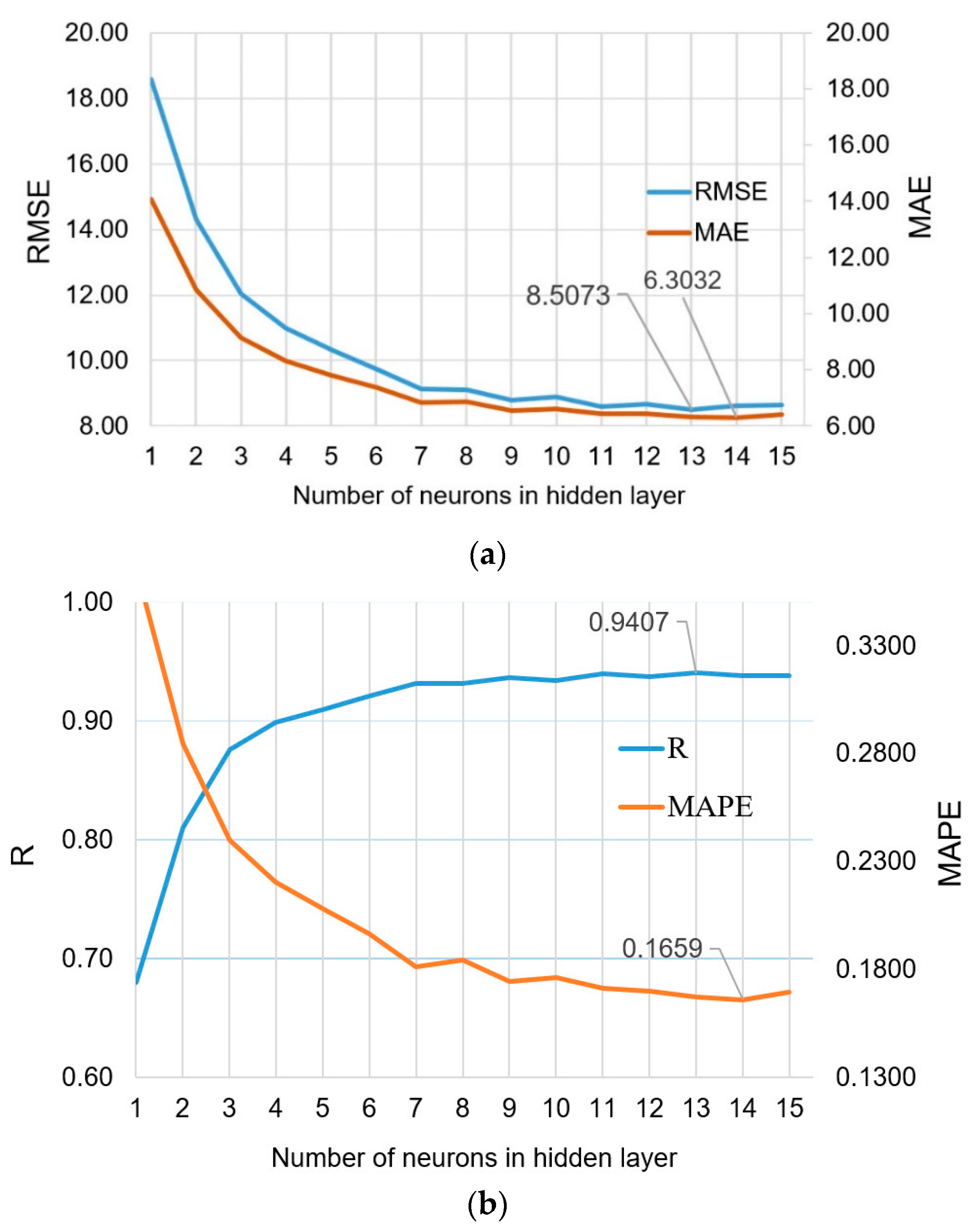
| NN 8-13- 1 | 8.5073 | 6.3133 | 0.1669 | 0.9407 |
| NN 8-14- 1 | 8.6289 | 6.3032 | 0.1659 | 0.9381 |
| Ensamble | 5.7858 | 4.1518 | 0.1098 | 0.9705 |
| GP exponential | 8.3622 | 6.0671 | 0.1713 | 0.9441 |
| GP Sq.exponential | 7.2756 | 5.4373 | 0.1492 | 0.9573 |
| GP matern 3/2 | 7.3460 | 5.3685 | 0.1494 | 0.9565 |
| GP matern 5/2 | 7.2130 | 5.2829 | 0.1470 | 0.9581 |
| GP Rat. quadratic | 7.2162 | 5.3151 | 0.1470 | 0.9580 |
| GP ARD exponential | 8.2035 | 5.2744 | 0.1183 | 0.9505 |
| GP ARD Sq. exponential | 8.3531 | 5.2521 | 0.1188 | 0.9483 |
| GP ARD matern 3/2 | 9.3960 | 5.0817 | 0.1045 | 0.9351 |
| GP ARD matern 5/2 | 6.9976 | 4.7886 | 0.1127 | 0.9652 |
| GP ARD Rat. quadratic | 6.7137 | 4.6157 | 0.1082 | 0.9681 |
Disclaimer/Publisher’s Note: The statements, opinions and data contained in all publications are solely those of the individual author(s) and contributor(s) and not of MDPI and/or the editor(s). MDPI and/or the editor(s) disclaim responsibility for any injury to people or property resulting from any ideas, methods, instructions or products referred to in the content. |
© 2023 by the authors. Licensee MDPI, Basel, Switzerland. This article is an open access article distributed under the terms and conditions of the Creative Commons Attribution (CC BY) license (https://creativecommons.org/licenses/by/4.0/).
Share and Cite
Kovačević, M.; Hadzima-Nyarko, M.; Grubeša, I.N.; Radu, D.; Lozančić, S. Application of Artificial Intelligence Methods for Predicting the Compressive Strength of Green Concretes with Rice Husk Ash. Mathematics 2024, 12, 66. https://doi.org/10.3390/math12010066
Kovačević M, Hadzima-Nyarko M, Grubeša IN, Radu D, Lozančić S. Application of Artificial Intelligence Methods for Predicting the Compressive Strength of Green Concretes with Rice Husk Ash. Mathematics. 2024; 12(1):66. https://doi.org/10.3390/math12010066
Chicago/Turabian StyleKovačević, Miljan, Marijana Hadzima-Nyarko, Ivanka Netinger Grubeša, Dorin Radu, and Silva Lozančić. 2024. "Application of Artificial Intelligence Methods for Predicting the Compressive Strength of Green Concretes with Rice Husk Ash" Mathematics 12, no. 1: 66. https://doi.org/10.3390/math12010066
APA StyleKovačević, M., Hadzima-Nyarko, M., Grubeša, I. N., Radu, D., & Lozančić, S. (2024). Application of Artificial Intelligence Methods for Predicting the Compressive Strength of Green Concretes with Rice Husk Ash. Mathematics, 12(1), 66. https://doi.org/10.3390/math12010066