Feedback Stabilization Applied to Heart Rhythm Dynamics Using an Integro-Differential Method

Abstract

In this paper, we applied a chaos control method based on integro-differential equations for stabilization of an unstable cardiac rhythm, which is described by a variation of the modified Van der Pol equation. Chaos control with this method may be useful for stabilization of irregular heartbeat using a small perturbation. This method differs from other stabilization strategies by the absence of adjustable parameters and the lack of rough approximations in determining control functions whose control parameters are fixed by the properties of the unstable system itself.

1. Introduction

Unlike a mechanical clock, even healthy heartbeats can be irregular. Regular and random heart rhythms can be associated with normal or pathological heart behavior [1,2,3,4,5,6]. Mathematical modeling is an important instrument in the study of the human organism helping to solve the difficult problems of human experimental research. Chaos and nonlinear dynamics investigation is a long-standing approach in various disciplines such as physics, chemistry, engineering, biology, medicine, and economics. The Van der Pol equation is a good phenomenological model of the dynamics of cardiovascular rhythms due to the similarity of qualitative features of heart dynamics for all individuals [7,8,9,10,11,12]. Chaos control is critically relevant in many circumstances in terms of preventing catastrophes and collapse in a dynamic system.

In [8], the chaos control method that was created by Pyragas was used. In this method, feedback consists of two control parameters, R and K, which are described in [8]. For each desired orbit, a selection of the correct control is needed to set. If the feedback provides small values of perturbation, a successful control is achieved. This choice is made by analyzing Lyapunov exponents of the corresponding orbit. After this stage, the control stage is performed, where the desired equations are stabilized. We note that in this article, successful control is only achieved when $R=0$, because in this case the time delay $\tau$ is equal to an integer number of periods; thus, the generality of this method is limited.

Among the variety of control techniques used in dynamical systems, there is a method of great theoretical and practical importance. It is the analysis of the stability of the equations using process history. Our results on the stabilization are obtained on the basis of this approach [13,14,15,16].

We also notice other important works in which delay is involved. For example, in [17], it was shown how the frequency of an oscillation determines the exact form of the control for suppressing the oscillation through feedback controls with time delays. In [18], an adaptive control scheme is presented with feedback delay to achieve elimination of synchronization in a large population of coupled and synchronized oscillators. We also notice that [19] uses delay to eliminate synchronization of coupled neurons adaptively by using feedback coupling with heterogeneous delays.

Chaotic dynamics and stochastic dynamics share some similarities regarding the erratic behavior of the dynamical variables, but they arise from fundamentally different mechanisms. In chaotic dynamics, chaos is deterministic, meaning that the system’s behavior is entirely determined by its initial conditions. However, chaotic systems are highly sensitive to initial conditions, resulting in complex and seemingly random behavior over time. Small changes in initial conditions can lead to drastically different outcomes. Stochastic systems, on the other hand, involve randomness and inherent unpredictability. Random processes, such as Brownian motion, introduce uncertainty that is not based on sensitivity to initial conditions. However, the parameters of a chaotic nonlinear equation can be thought of as stochastic variables which have an average value but can also deviate from this random value. Our stabilization technique is not sensitive to the value of some of the parameters; this is shown mathematically and also demonstrated by a numerical experiment.

2. Formulation of a Stabilization Problem

It is known [20] that, with a very small external force u, one can obtain various types of regular behavior of process x, which is described, for example, by equation

$$x^{\prime }\left(t\right)-ax\left(t\right)+Ru\left(t\right)=0,$$

(1)

in which a and R are some real constants. Various approaches to stabilization are based on a delayed feedback control scheme [21], where dynamical time-delayed feedback control is used. This scheme includes control signal $u\left(t\right)$ generated by the difference between the current state $x\left(t\right)$ and the previous state $x(t-\tau )$ of the system.

Another suggestion of feedback stabilization of control systems with process history is the integro-differential equation method. Integro-differential equations can be considered as a class of equations with unbounded memory. The stability of these equations was studied, for example, in [13,22].

It is quite reasonable to choose control $u\left(t\right)$ in the form

$$u\left(t\right)={\int }_0^{t}k(t,s)x\left(s\right)ds.$$

(2)

The method proposed below avoids difficulties associated with the use of control in the integral form of Equation (2) but without loosing its advantages [13,15]. This is first demonstrated by a simple example.

Example 1. 

We consider the following scalar equation:

$$x^{\prime }\left(t\right)=a_{1}x\left(t\right),$$

(3)

$a_1$ is a constant. If $a_1>0,$ then the solution of Equation (3), $x=0$, is unstable. Let us now consider the following equation as a model to study the stability of an integro-differential equation:

$$x^{\prime }\left(t\right)-a_{1}x\left(t\right)+{\int }_0^{t}k(t,s)x\left(s\right)ds=0,t\in [0,+\infty ).$$

(4)

Thus, $R=1$ and $a=a_1$. According to the reduction method [13], we assume that

$$k(t,s)=\alpha e^{-\beta (t-s)},$$

(5)

where α and β are the control parameters to be specified later. The value of those parameters is dependent on the parameters of the problem at hand, which is explained in detail below for specific examples. Defining the control function as

$$u\left(t\right)={\int }_0^t{e}^{-\beta (t-s)}x\left(s\right)ds,$$

(6)

we obtain Equation (4) in the form

$$x^{\prime }\left(t\right)-a_{1}x\left(t\right)+\alpha u\left(t\right)=0.$$

(7)

In accordance with the Leibniz rule for differentiation under the integral sign of the form ${\displaystyle \frac{d}{dt}}{\int }_{a\left(t\right)}^{b\left(t\right)}f(t,s)ds$, we obtain the expression for $u^{\prime }\left(t\right)$:

$$u^{\prime }\left(t\right)=-\beta {\int }_0^t{e}^{-\beta (t-s)}x\left(s\right)ds+e^{-\beta (t-t)}x\left(t\right)-0=-\beta u\left(t\right)+x\left(t\right).$$

(8)

Using the Leibniz rule, we can write Equation (7) in the form

$$\left\{\begin{array}{c}{x}^{\prime }\left(t\right)=a_{1}x\left(t\right)-\alpha u\left(t\right),\hfill \\ u^{\prime }\left(t\right)=-\beta u\left(t\right)+x\left(t\right),t\in [0,+\infty ),\hfill \\ u\left(0\right)=0.\hfill \end{array}\right.$$

(9)

The characteristic equation of System (9) is the following:

$${\lambda }^2+(\beta -a_1)\lambda +\alpha -\beta a_1=0.$$

(10)

Conditions

$$\beta -a_1>0and\alpha -\beta a_1>0$$

(11)

are necessary and sufficient for the exponential stability of System (9). If Conditions (11) are fulfilled, then solution $x\left(t\right)=0$ of System (9) is exponentially stable.

The main advantages of this method are as follows:

• As noted above, small values of the control signal are needed (compared to the stabilized functions) when stabilization is achieved.
• Using control function $u\left(t\right)$ in Form (6) in which all the history of process $x\left(t\right)$ is taken into account, we reduce the study of the integro-differential system of the order n to the analysis of the $n+1$ order system of ordinary differential equations [13].
• It differs from other stabilization schemes by the absence of adjustable parameters and rough approximations in determining the control function. Control parameters $\alpha$ and $\beta$ are determined by the properties of the unstable system itself.

We successfully used this method to stabilize several physical systems [14,23,24]. The class of systems being considered is non-linear (and linear) ordinary differential equations of any order. What needs to be achieved is stabilization of those systems such that chaos is controlled. Of course, for high-order equations, the characteristic polynomial is high order as well. The ordinary differential equation mentioned below is an example of stabilizing a non-linear differential equation of the second order.

3. Mathematical Model of Heart Rythm Dynamics Based on a Modified Van der Pol Equation

3.1. Problem Statement

Grudzinski and Zebrowski proposed a modification of the classic Van der Pol equation [9]. This new model allows one the simulation of important physiological characteristics of a natural cardiac pacemaker, the signal of which is denoted by $x\left(t\right)$. We use symbols $x^{\prime }$ and $x^{″}$ for the first and second derivatives of this signal, respectively. Standard SI units of $x\left(t\right)$ are millivolts, t is measured in seconds. The suggested model is represented by the following equation [8]:

$$x^{″}+a(x-v_1)(x-v_2)x^{\prime }+\frac{x(x+d)(x+e)}{ed}=F\left(t\right),$$

(12)

where a modifies the form of the impulse which in turn changes the time in which the heart is stimulated, $v_1$ and $v_2$ make up an asymmetric term that replaces the damping part that exists in the classical van der Pol equation, e regulates the period of atrial or ventricular contraction period, d is a parameter that arises when the harmonic forcing of classic equation is replaced by a cubic term and $F\left(t\right)$ is an external forcing. In the following, we choose

$$F\left(t\right)=Asin\left(\omega t\right),$$

(13)

in which A is the amplitude of the force and $\omega$ is its angular frequency. Hence, the pacemaker (Equation (12)) is described by the following system of first-order ordinary differential equations:

$$\left\{\begin{array}{c}{x}^{\prime }\left(t\right)=y\left(t\right),\hfill \\ {\displaystyle y^{\prime }\left(t\right)+a(x\left(t\right)-v_1)(x\left(t\right)-v_2)y\left(t\right)+\frac{x\left(t\right)\left(x\right(t)+d)\left(x\right(t)+e)}{ed}}\hfill \\ -Asin\left(\omega t\right)=0.\hfill \end{array}\right..$$

(14)

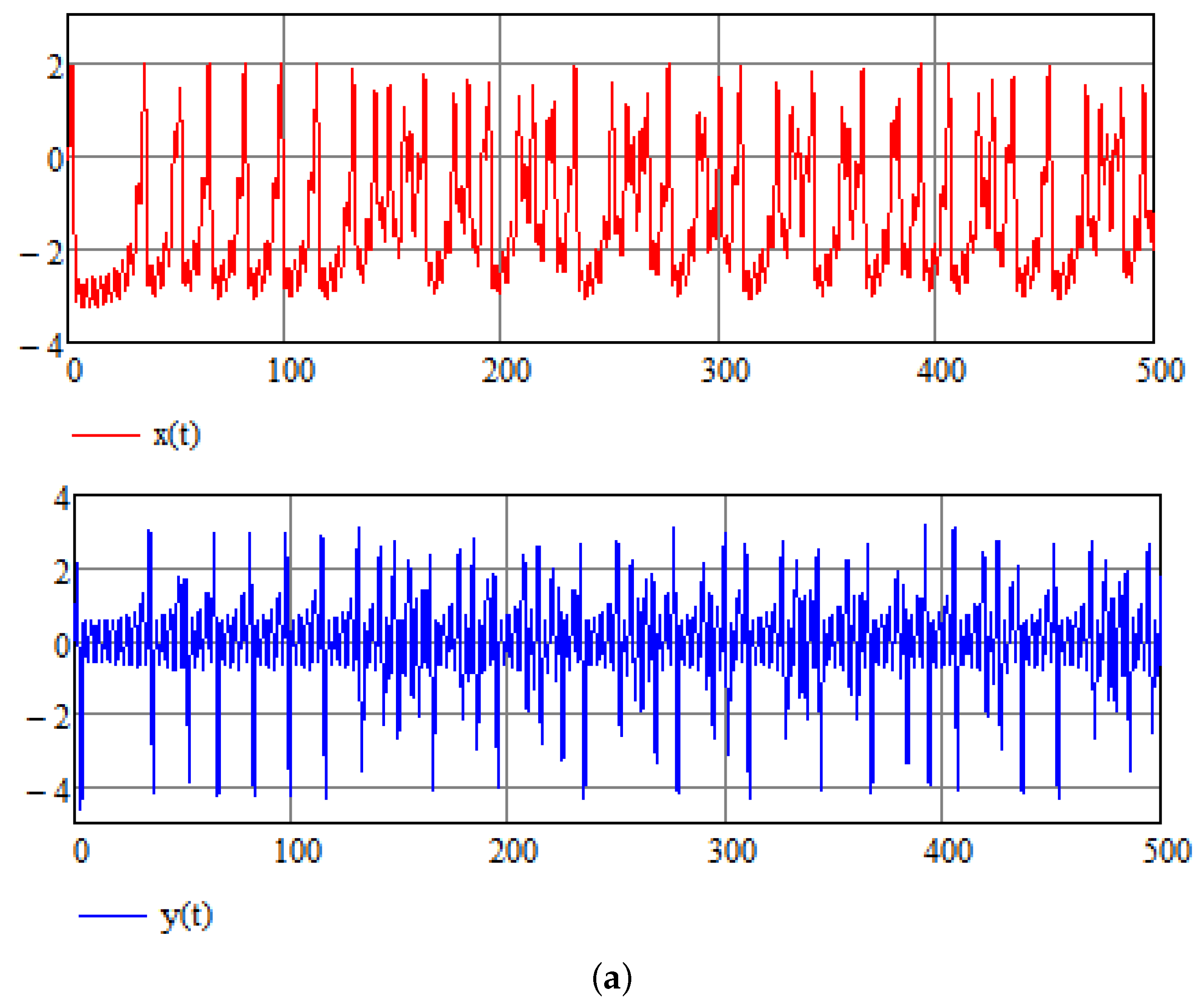
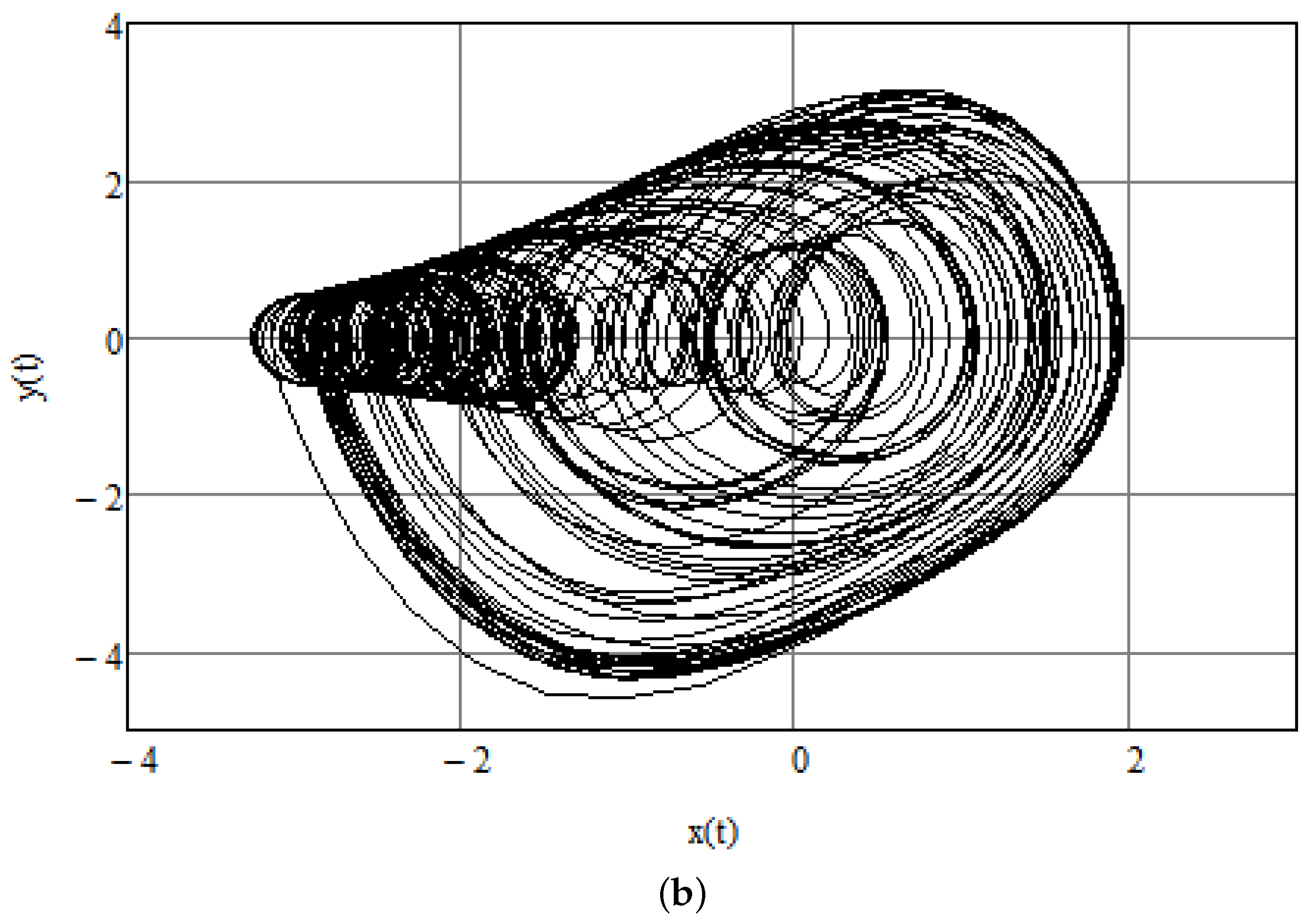
Chaotic reactions of the cardiac system may be related to abnormal physiological functioning such as ventricular fibrillation, which is one of the most dangerous cardiac arrhythmias [25,26]. Various parameters are supposed to represent this type of pathology. In accordance with [8], the following parameters are assumed: $a=0.5, v_1=0.97, v_2=-1$, $d=3, e=6, A=2.5$ and $\omega =1.9$. The chaotic reaction can be seen in Figure 1a,b that show time history and phase space for the initial condition $\left[x\right(0),y(0\left)\right]=[-0.1,0.025]$. As for the numerical method, the program Mathcad is used, which relies on the standard Runge–Kutta method. The RK4 method used is a fourth-order method, meaning that the local truncation error is of the order of $O\left(h^5\right)$ while the total accumulated error is of the order of $O\left(h^4\right)$.

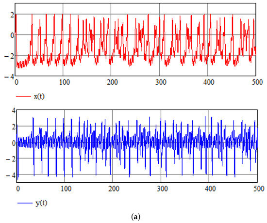
Figure 1. (a) Chaotic pacemaker activity. Time dependence for $0⩽t⩽500$. (b) Chaotic pacemaker activity. Phase space. Time interval $0⩽t⩽1000$.

In the next subsection, we attempt the control of a chaotic behavior using a control function.

3.2. Proposed Method

Let us use control $u\left(t\right)$ in the form

$$u\left(t\right)=\underset{0}{\overset{t}{\int }}{e}^{-\beta (t-s)}y\left(s\right)ds,$$

(15)

in which all the history of process $y\left(t\right)$ is taken into account [13]. We apply stabilization by a feedback delay control signal to System (14) assuming that control signal $u\left(t\right)$ acts only in the second equation:

$$\left\{\begin{array}{c}{x}^{\prime }\left(t\right)=y\left(t\right),\hfill \\ {\displaystyle y^{\prime }\left(t\right)+a(x\left(t\right)-v_1)(x\left(t\right)-v_2)y\left(t\right)+\frac{x\left(t\right)\left(x\right(t)+d)\left(x\right(t)+e)}{ed}}\hfill \\ -Asin\left(\omega t\right)+\alpha u\left(t\right)=0,\hfill \\ u^{\prime }\left(t\right)-y\left(t\right)+\beta u\left(t\right)=0\hfill \end{array}\right..$$

(16)

The corresponding homogeneous linearized system (linearized around $x\left(0\right)=y\left(0\right)=u\left(0\right)=0$) can be written as follows [14]:

$$\left\{\begin{array}{c}{x}^{\prime }\left(t\right)-y\left(t\right)=0,\hfill \\ y^{\prime }\left(t\right)+a{v}_1{v}_{2}y\left(t\right)+x\left(t\right)+\alpha u\left(t\right)=0,\hfill \\ u^{\prime }\left(t\right)+\beta u\left(t\right)-y\left(t\right)=0.\hfill \end{array}\right.$$

(17)

The characteristic equation of System (17) is

$${\lambda }^3+{\lambda }^2\left(\beta +a{v}_1{v}_2\right)+\lambda \left(\alpha +1+a{v}_1{v}_2\beta \right)+\beta =0.$$

(18)

According to Routh–Hurwitz conditions (see, for example, [27]), inequalities

$$\left\{\begin{array}{c}\beta >0,\hfill \\ \beta +a{v}_1{v}_2>0,\hfill \\ \alpha +1+a{v}_1{v}_2\beta >0,\hfill \\ \left(\beta +a{v}_1{v}_2\right)\left(\alpha +1+a{v}_1{v}_2\beta \right)-\beta >0\hfill \end{array}\right.$$

(19)

are necessary and sufficient conditions for the negativity of the real parts of the roots of characteristic Equation (18). From (18), we obtain

$${\displaystyle \beta >0,-a{v}_1{v}_1<\beta <-\frac{\alpha +1}{a{v}_1{v}_2};}$$

(20)

$$\left(a{v}_1{v}_2\right){\beta }^2+\left(\alpha +{\left(a{v}_1{v}_2\right)}^2\right)\beta +\left(a{v}_1{v}_2\right)\left(1+\alpha \right)>0.$$

(21)

The roots of Polynomial (21) are

$${\beta }_{1,2}=\frac{-\left(\alpha +{\left(a{v}_1{v}_2\right)}^2\right)\pm \sqrt{{\left({\left(a{v}_1{v}_2\right)}^2-\alpha \right)}^2-4{\left(a{v}_1{v}_2\right)}^2}}{2a{v}_1{v}_2}.$$

(22)

Finally, we obtain the following inequalities:

$$\begin{array}{c}{\left({\left(a{v}_1{v}_2\right)}^2-\alpha \right)}^2-4{\left(a{v}_1{v}_2\right)}^2>0\Rightarrow \alpha >{\left(a{v}_1{v}_2\right)}^2-2a{v}_1{v}_2,\\ \beta >0,\beta <-\frac{\alpha +1}{a{v}_1{v}_2},\\ \beta >\frac{-\left(\alpha +{\left(a{v}_1{v}_2\right)}^2\right)-\sqrt{{\left({\left(a{v}_1{v}_2\right)}^2-\alpha \right)}^2-4{\left(a{v}_1{v}_2\right)}^2}}{2a{v}_1{v}_2}.\end{array}$$

(23)

We can stabilize System (16) in its second equation by integral feedback control (15) if we choose positive parameters $\alpha$ and $\beta$ such that

$$\begin{array}{c}\alpha >{\left(a{v}_1{v}_2\right)}^2-2a{v}_1{v}_2,\\ -\frac{\alpha +1}{a{v}_1{v}_2}>\beta >\frac{-\left(\alpha +{\left(a{v}_1{v}_2\right)}^2\right)-\sqrt{{\left({\left(a{v}_1{v}_2\right)}^2-\alpha \right)}^2-4{\left(a{v}_1{v}_2\right)}^2}}{2a{v}_1{v}_2}.\end{array}$$

(24)

The selection of control parameters alpha and beta is not unique; rather, it is defined by inequalities depending on the system parameters which must be satisfied.

4. Numerical Results of Numerical Stabilization of a Modified Van der Pol Equation

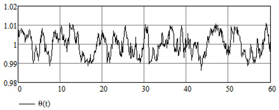
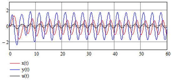
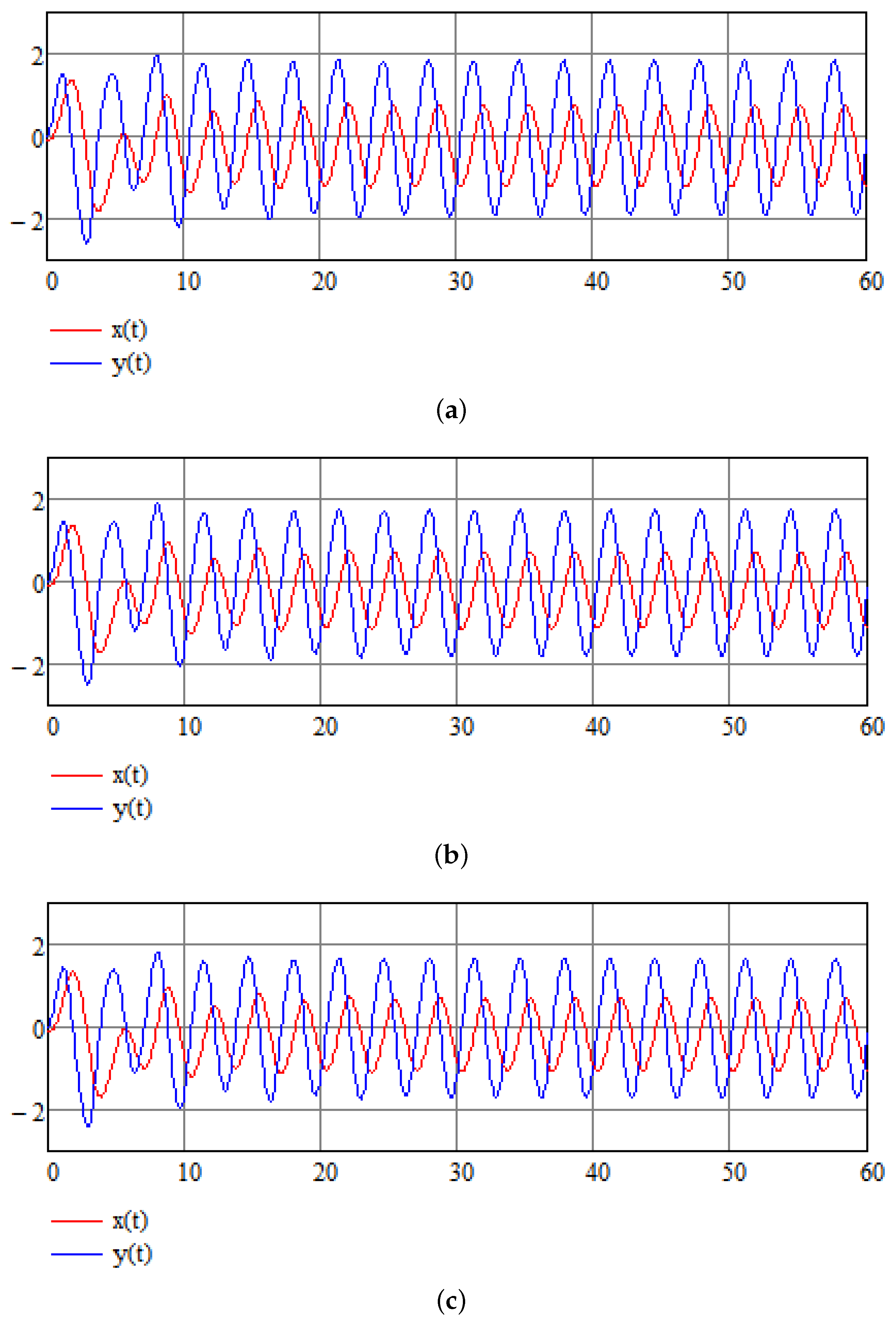
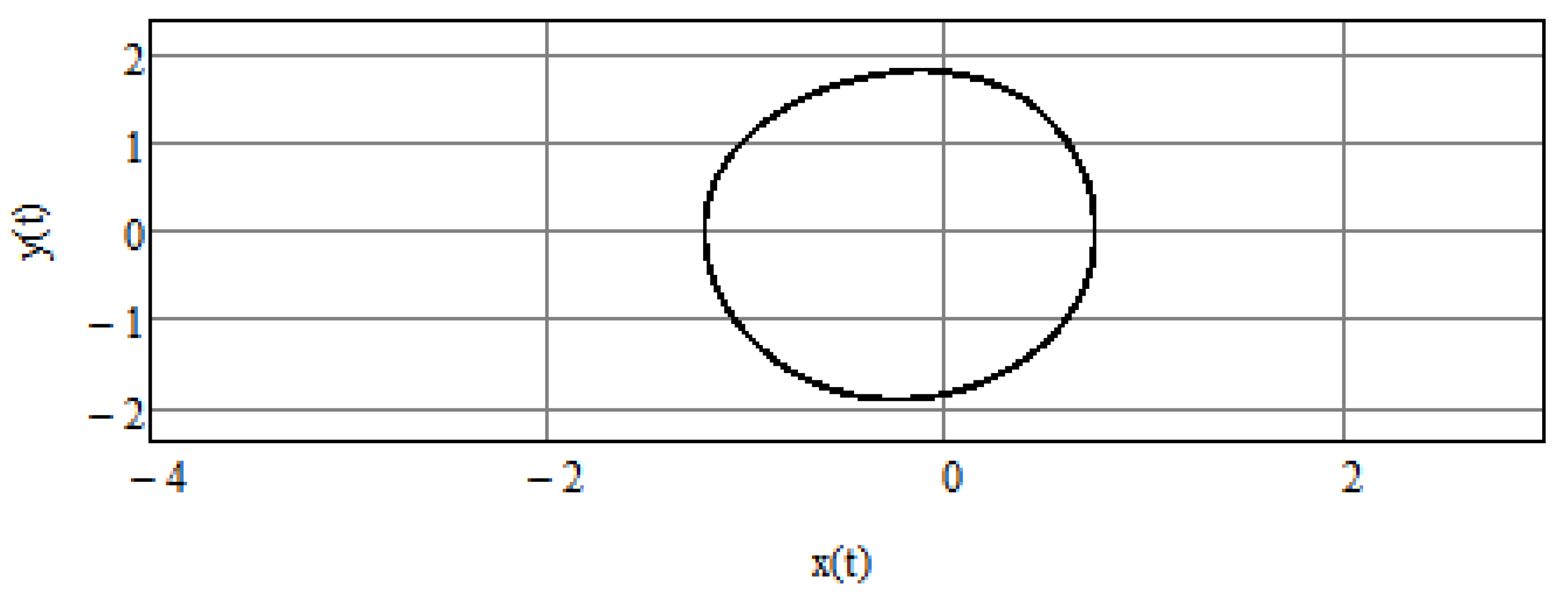
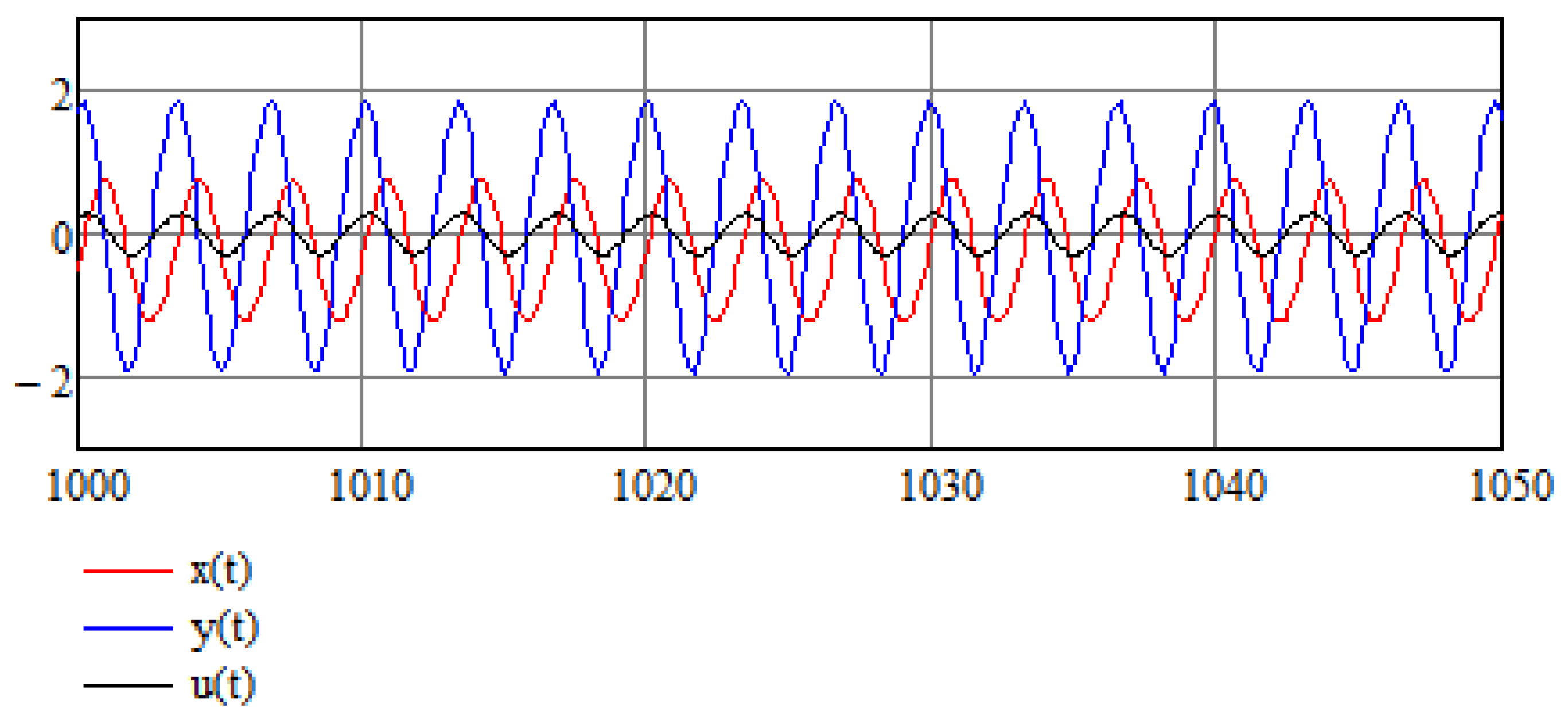
Below, we represent the results of stabilization of chaotic System (16). By stabilization we mean that system variables $x\left(t\right),y\left(t\right)$ change periodically in an orderly oscillatory fashion and do not behave chaotically (this does not mean that any of the variables approach zero for long enough durations). Stabilization was achieved by the method based on the integro-differential equations technique presented above. Parameters of the system are as described in the previous section. The solution of this set of equation is performed over time interval $0⩽t⩽$ 10,000. Initial conditions $x\left(0\right)=-0.1,y\left(0\right)=0.025,u\left(0\right)=0.0$. $x\left(t\right)$ and $y\left(t\right)$ are given in Figure 2 for the first sixty time units, showing how quickly the system is stabilized. We use three different values of $\alpha$ and $\beta$: $\alpha =6.5,\beta =6.3$ in Figure 2a, $\alpha =10.5,\beta =10.3$ in Figure 2b, and $\alpha =20.5,\beta =20.3$ in Figure 2c, showing that the choice of the stabilizing parameters is not unique and stabilization occurs provided that Equation (24) is satisfied. The solution of this set of equations is performed over time interval $0⩽t⩽10,000$. Figure 3 shows the parametric plot of $x\left(t\right),y\left(t\right)$ and an ellipse-like plot obtained for a time interval $1000⩽t⩽1500$, which attests to the stability of the system even after a long time interval. Figure 4 compares control function $u\left(t\right)$ to original signals $x\left(t\right)$ and $y\left(t\right)$ showing how minute the intervention is that is required to achieve stability (which may have life-saving effects).

Figure 2. (a) Numerical results of the stabilization of a modified Van der Pol Equation (16) for $\alpha =6.5,\beta =6.3$. (b) Numerical results of the stabilization of a modified Van der Pol Equation (16) for $\alpha =10.5,\beta =10.3$. (c) Numerical results of the stabilization of a modified Van der Pol Equation (16) for $\alpha =20.5,\beta =20.3$.

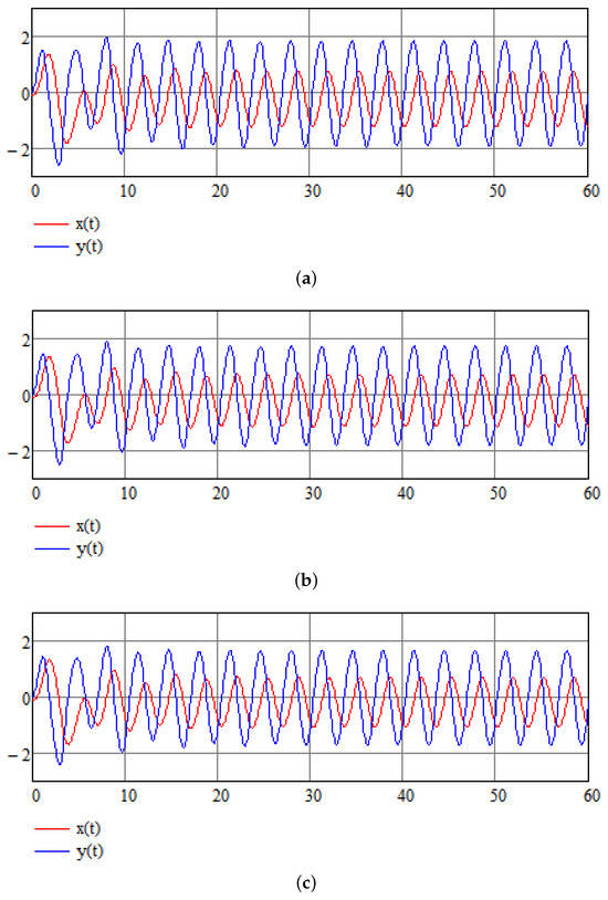
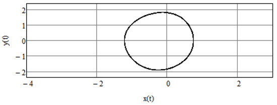
Figure 3. The phase trajectory of the solution of System (16) in the $(x,y)$ plane; time interval is taken to be $1000⩽t⩽1500$.

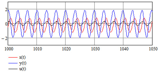
Figure 4. Control function $u\left(t\right)$ compared to the stabilized process $x\left(t\right),y\left(t\right)$.

5. Stochastic Perspective

5.1. Introductory Remarks

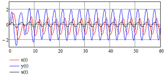
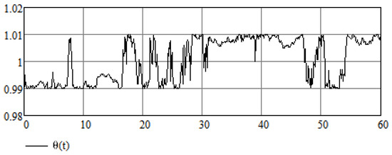
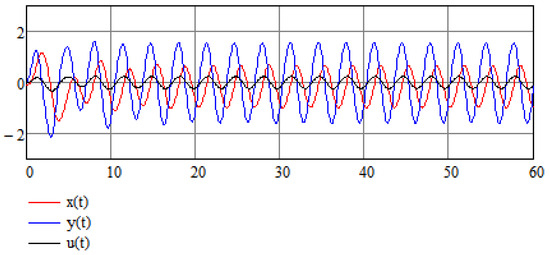
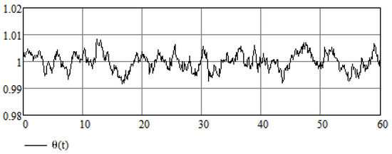
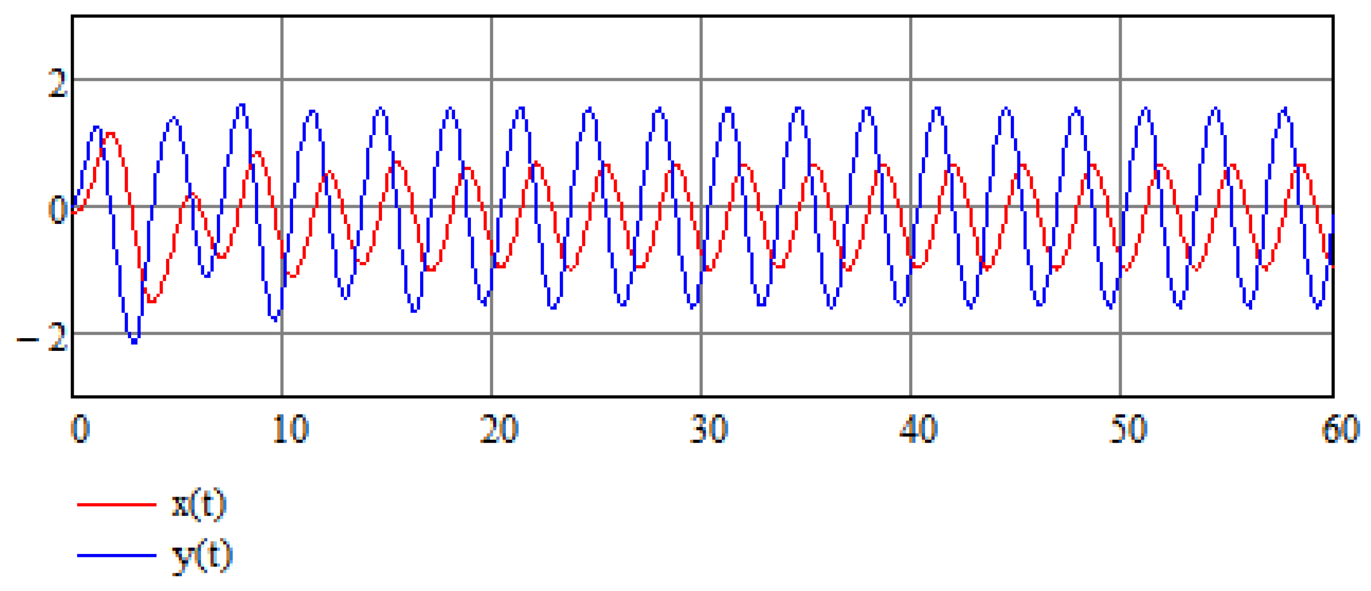
Let us suppose that Equation (14) is an equation in which variable A is a random variable which results from some random process; in this case, $A=2.5$ can be thought of as an average value of a random variable, that is, $E\left[A\right]=2.5$. Now, according to the analysis of Equation (24), the value of A does not affect the stabilization of the system, hence A need not be equal to its average value for the stabilization method to work. This is also demonstrated in Figure 5 and Figure 6 for the cases in which the random variable takes values $A=2$ and $A=3$, respectively.

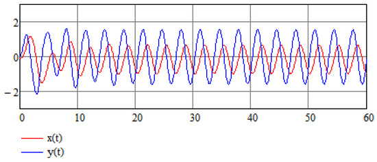
Figure 5. Numerical results of the stabilization of a modified Van der Pol Equation (16) for $A=2$.

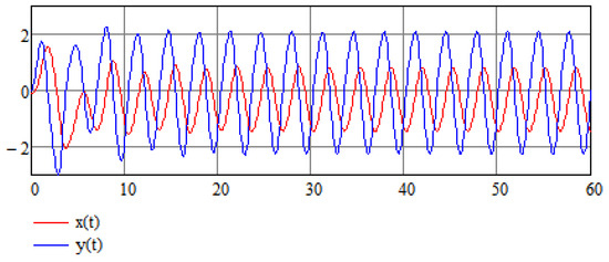
Figure 6. Numerical results of the stabilization of a modified Van der Pol Equation (16) for $A=3$.

5.2. Additional Examples

Further, more complicated examples are considered.

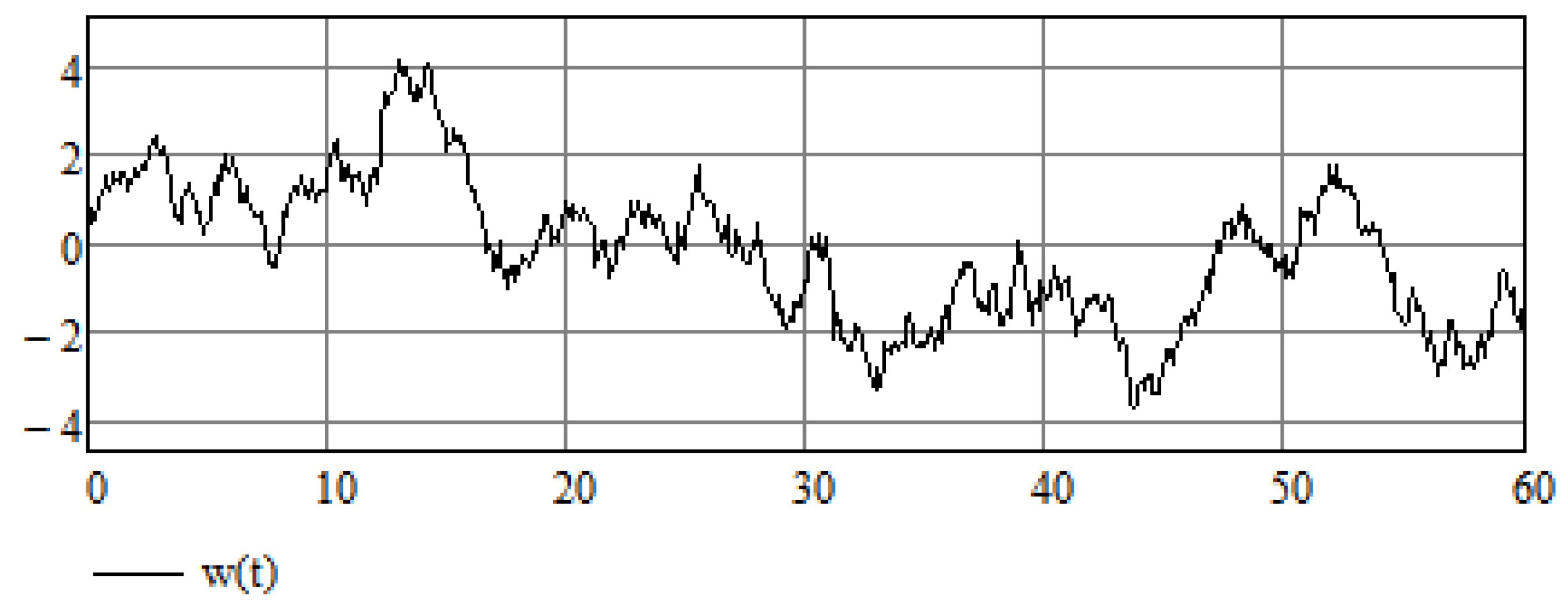
We let $w\left(t\right)$ be the standard Wiener process: $w\left(0\right)=0$, $w\left(t\right)$ has independent increments, $w\left(t\right)-w\left(s\right)\sim \mathcal{N}(0,t-s)$ for $0⩽s<t$, where $\mathcal{N}$ denotes Gaussian distribution. It can be simulated on the interval $[0,T]$ with step size h as follows:

$$w_0=0,w_{i+1}=w_i+\sqrt{h}{\zeta }_i,i=0,1,\dots ,N-1,N=T/h,$$

where $T/h$ is the integer value and ${\zeta }_i$ are independent random variables with standard Gaussian distribution.

A depiction of a sample path of the Wiener process is given in Figure 7.

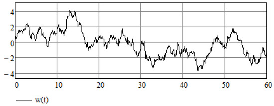
Figure 7. A sample path of the Wiener process $w\left(t\right)$.

Next, we can use external forcing $F\left(t\right)=A\theta \left(t\right)sin\left(\omega t\right)$ instead of $F\left(t\right)=Asin\left(\omega t\right)$ in Equation (12), where $\theta \left(t\right)$ is a random process that takes values around one, for example, $\theta \left(t\right)\in [1-\nu ,1+\nu ]$, where $\nu =0.01$. In this case, the uncontrolled equations take the form

$$\left\{\begin{array}{c}{x}^{\prime }\left(t\right)=y\left(t\right),\hfill \\ {\displaystyle y^{\prime }\left(t\right)+a(x\left(t\right)-v_1)(x\left(t\right)-v_2)y\left(t\right)+\frac{x\left(t\right)\left(x\right(t)+d)\left(x\right(t)+e)}{ed}}\hfill \\ -A\theta \left(t\right)sin\left(\omega t\right)=0\hfill \end{array}\right.,$$

(25)

and the controlled equations take the form

$$\left\{\begin{array}{c}{x}^{\prime }\left(t\right)=y\left(t\right),\hfill \\ {\displaystyle y^{\prime }\left(t\right)+a(x\left(t\right)-v_1)(x\left(t\right)-v_2)y\left(t\right)+\frac{x\left(t\right)\left(x\right(t)+d)\left(x\right(t)+e)}{ed}}\hfill \\ -A\theta \left(t\right)sin\left(\omega t\right)-\alpha u\left(t\right)=0,\hfill \\ u^{\prime }\left(t\right)-y\left(t\right)+\beta u\left(t\right)=0\hfill \end{array}\right..$$

(26)

Example 2. 

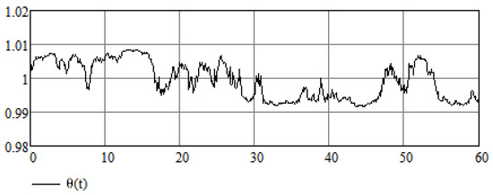
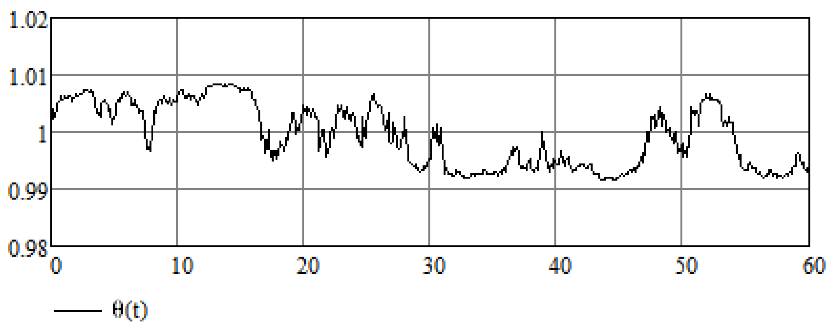
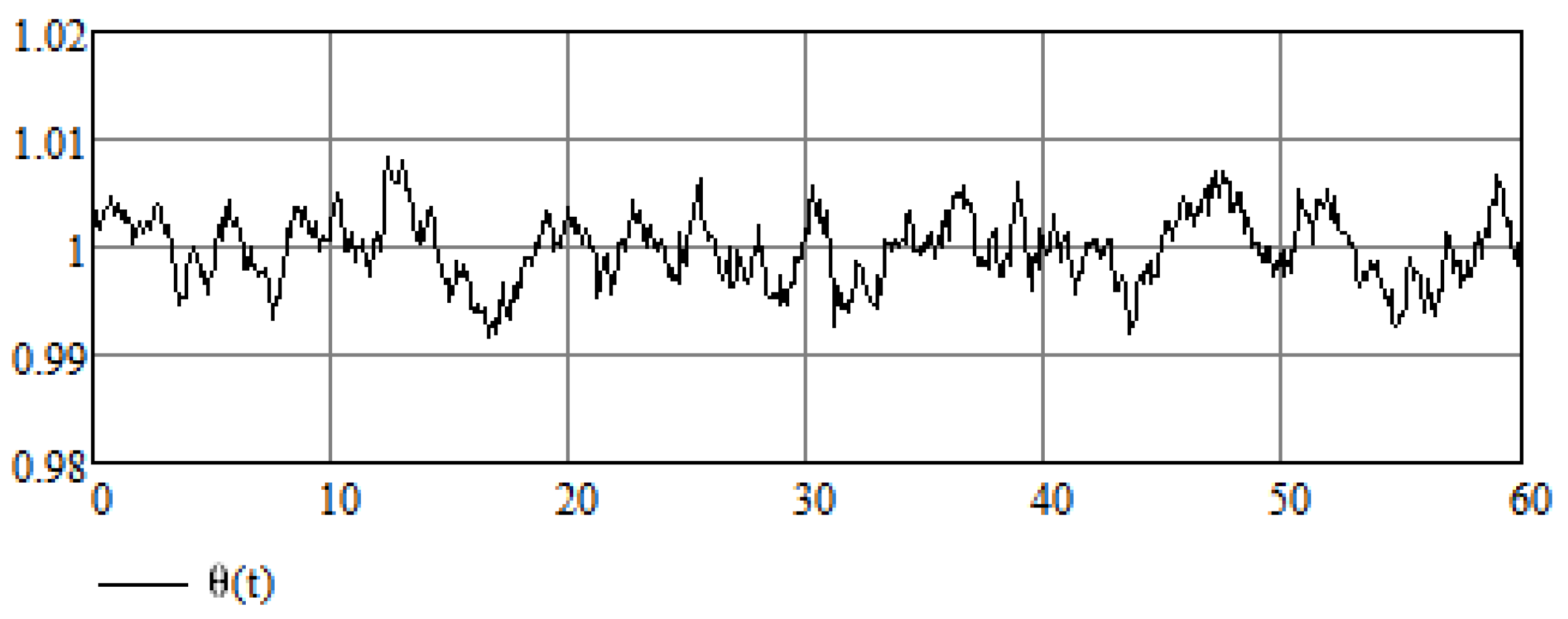
Following [28], let us define the random process $\theta \left(t\right)$ in terms of the Wiener process $w\left(t\right)$ mentioned above:

$$\theta \left(t\right)=1+\frac{2\nu }{\pi }arctanw\left(t\right).$$

Its sample path corresponding to the sample path of the Wiener process is depicted in Figure 8.

Figure 8. A sample path of the random process $\theta \left(t\right)$.

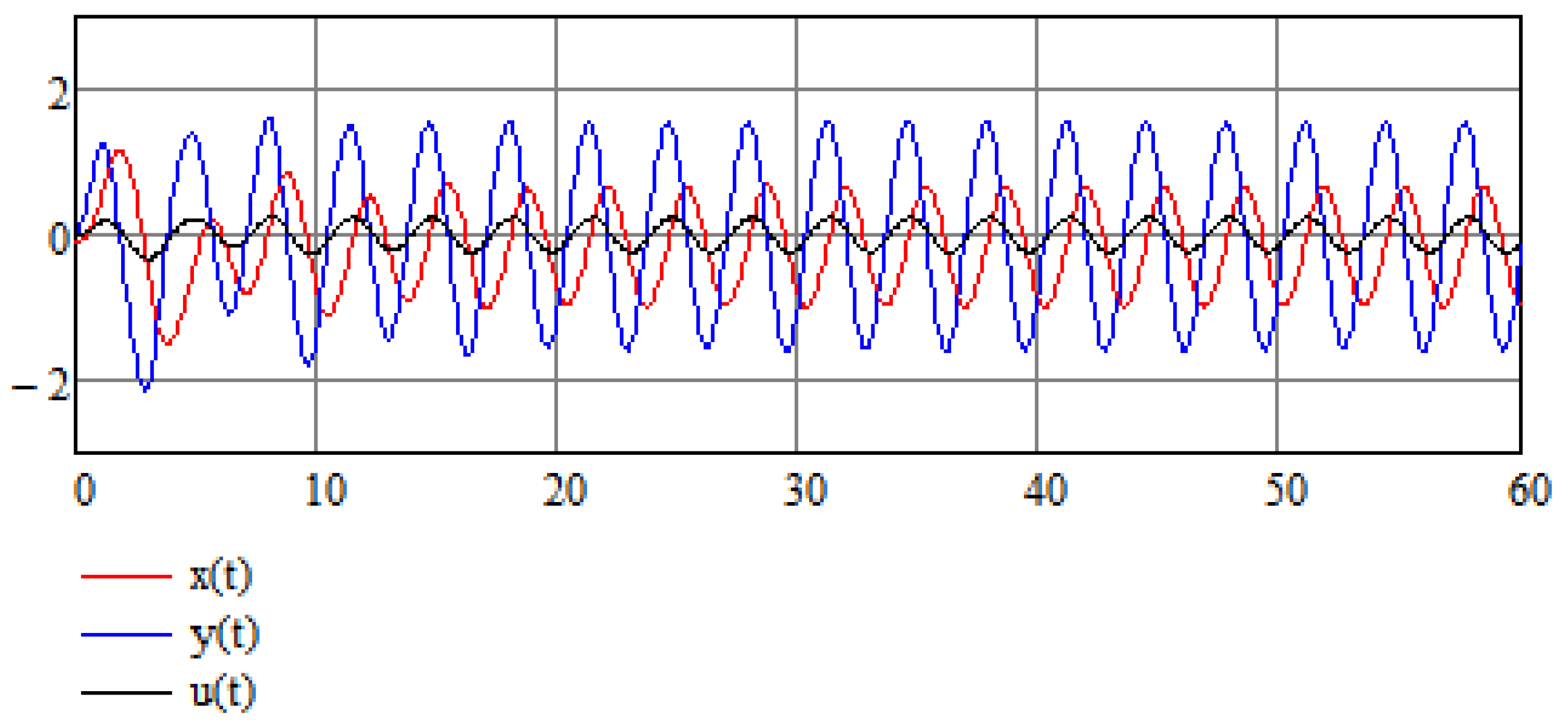
Despite stochastic forcing, our stabilization technique is still effective as can be seen in Figure 9, with a small correcting control function.

Figure 9. Numerical results of the stabilization of a modified stochastic Van der Pol Equation (25).

In the above, we use the same set of parameters as the original example with control parameters $\alpha =6.5,\beta =6.3$.

Example 3. 

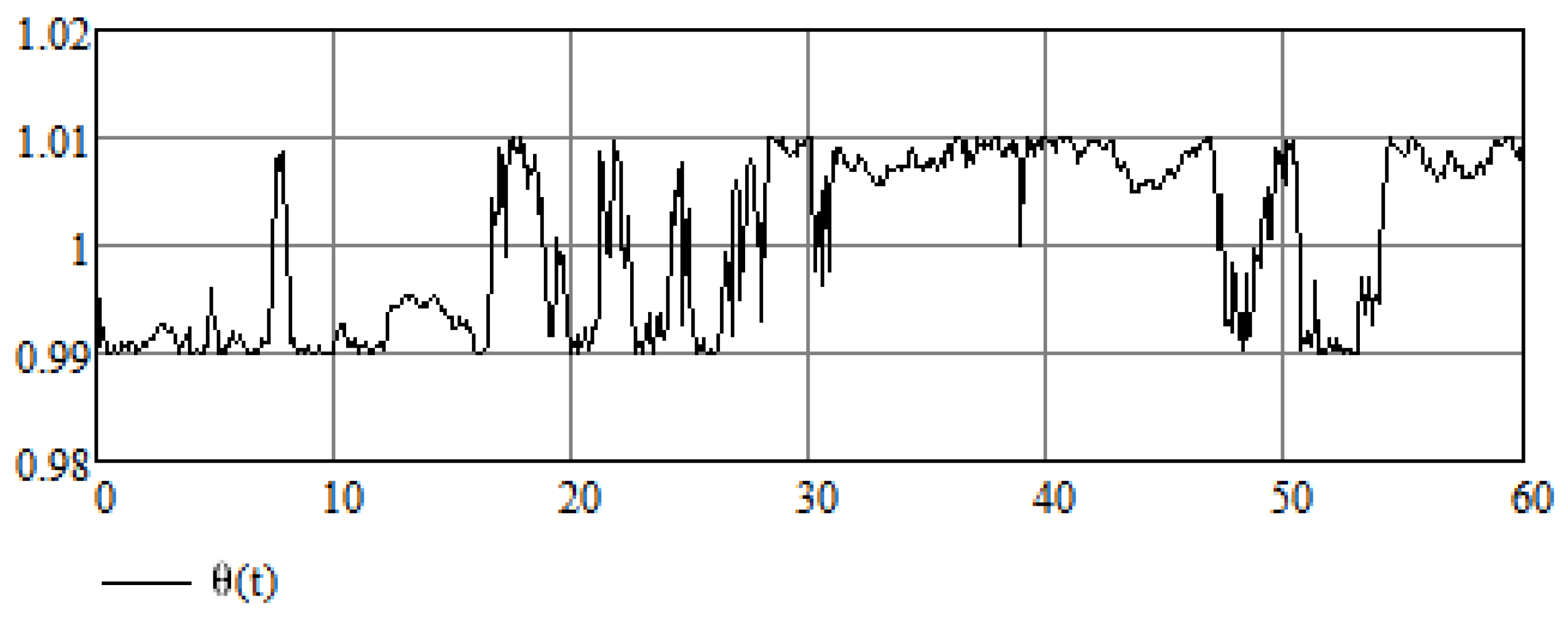
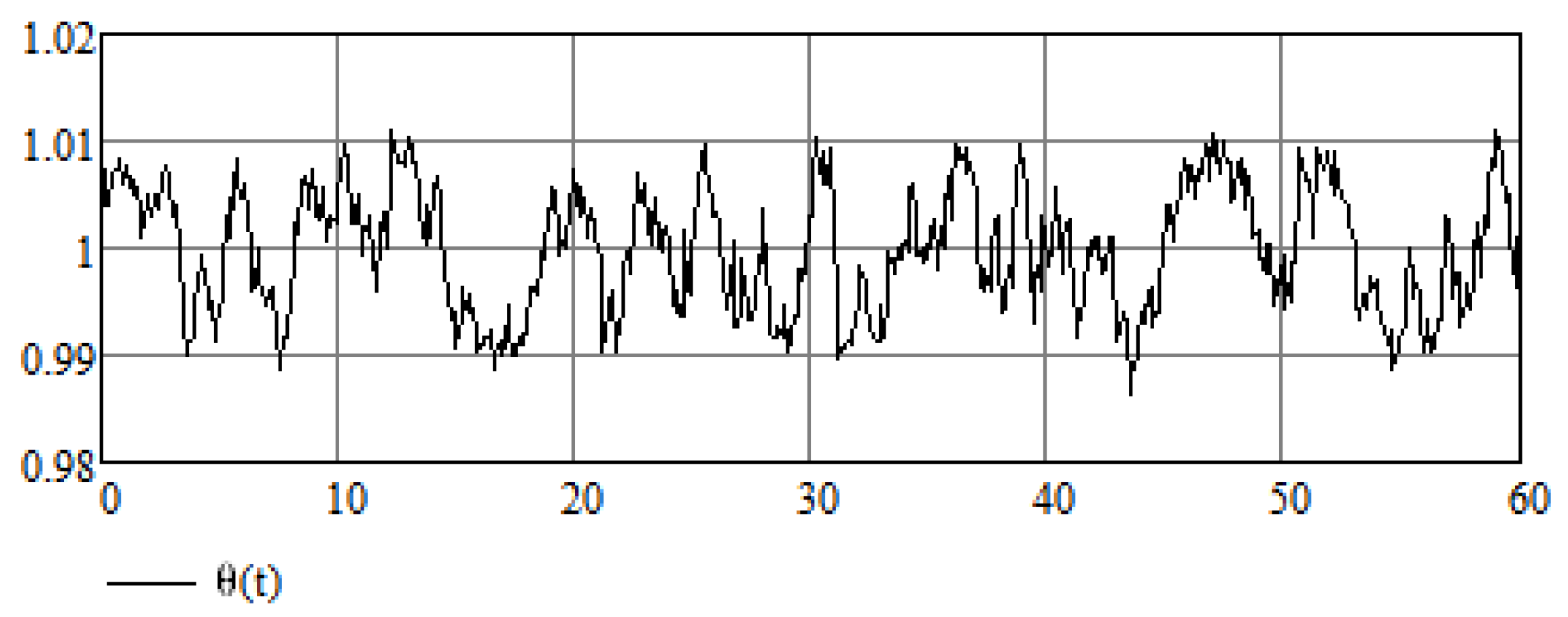
Another possible definition of the random process $\theta \left(t\right)$ is [28]

$$\theta \left(t\right)=1-2\nu \frac{w\left(t\right)}{1+w^2\left(t\right)}.$$

A sample path of this random process that corresponds to the sample path of the Wiener process is depicted in Figure 10.

Figure 10. A sample path of the random process $\theta \left(t\right)$.

Again, we use the same set of parameters as the original example but now take $A=2$, and take the control parameters to be $\alpha =6.5,\beta =6.3$. And again, we see that the control mechanism works efficiently as is evident from Figure 11.

Figure 11. Numerical results of the stabilization of a modified stochastic Van der Pol Equation (25).

Here, condition $\theta \left(t\right)\in [1-\nu ,1+\nu ]$ may be violated. The variance of $v\left(t\right)$ is ${(\nu /3)}^2$, and $v\left(t\right)$ has a zero mean. In fact, $\theta \left(t\right)\in [1-\nu ,1+\nu ]$ with probability $P\approx 0.997$.

Example 4. 

We now define

$$\theta \left(t\right)=1+v\left(t\right),$$

where $v\left(t\right)$ is the Ornstein–Uhlenbeck process that has Gaussian distribution [28]. The random process $v\left(t\right)$ is the solution to the Itô stochastic differential equation [29]:

$$dv\left(t\right)=-v\left(t\right)dt+\frac{\sqrt{2}\nu }{3}dw\left(t\right),v\left(0\right)\sim \mathcal{N}(0,{(1/3)}^2).$$

The sample paths of the Ornstein–Uhlenbeck process can be obtained by a numerical method, for example, by the Euler–Maruyama method. A sample path of random process $\theta \left(t\right)$ is depicted in Figure 12. It also corresponds to the sample path of the Wiener process.

Figure 12. A sample path of random process $\theta \left(t\right)$ related to the Ornstein–Uhlenbeck process.

Again, we use the same set of parameters as the original example, but now take $A=3$ and take the control parameters to be $\alpha =6.5,\beta =6.3$. We are not surprised to see that the control mechanism works efficiently also in this case as is evident from Figure 13.

Figure 13. Numerical results of the stabilization of a modified stochastic Van der Pol Equation (25).

Example 5. 

Finally, we define

$$\theta \left(t\right)=1+v\left(t\right),$$

where $v\left(t\right)$ has uniform distribution on interval $(-\nu ,\nu )$. This random process is the solution to the Itô stochastic differential equation [29]:

$$dv\left(t\right)=-v\left(t\right)dt+\sqrt{\left(v\right(t)+\nu )(\nu -v(t\left)\right)}dw\left(t\right),v\left(0\right)\sim \mathcal{R}(-\nu ,\nu ),$$

where $\mathcal{R}$ denotes uniform distribution.

The sample paths of the solution to this stochastic differential equation can also be obtained by the Euler–Maruyama method. Condition $\theta \left(t\right)\in [1-\nu ,1+\nu ]$ may be violated for the numerical solution. A sample path of random process $\theta \left(t\right)$ based on the above sample path of the Wiener process is depicted in Figure 14.

Figure 14. A sample path of random process $\theta \left(t\right)$ with uniform distribution.

We use the same set of parameters as the original example, but now take $A=2.25$, and the same control parameters, $\alpha =6.5,\beta =6.3$. We are not surprised to see that the control mechanism works efficiently also in this final case as is evident from Figure 15.

Figure 15. Numerical results of the stabilization of a modified stochastic Van der Pol Equation (25).

6. Discussion

In this article, we successfully stabilize unstable cardiovascular rhythm dynamics described by nonlinear oscillators of a modified Van der Pol equation by feedback control in an integral form. The main advantage of this method compared to the method applied by the authors of paper [8] is that we use control function $u\left(t\right)$ in the form (15) in which all the history of process $y\left(t\right)$ was taken into account, whereas these authors worked with the Wolf algorithm to analyze the Lyapunov exponents. This algorithm requires a big data set and works well with large amount of data (the order of several tens or hundreds), but may fail in situations with limited data [30]. In addition, the authors of work [31] revealed that the existence of Lyapunov exponents is a delicate matter for systems that are not conservative. In fact, in the situation of abstract dynamical systems, Barreira and Schmeling [32] claimed that the Lyapunov exponents often do not exist.

7. Conclusions

The novelty of the proposed stabilization method is that it can be formulated of a set of first-order differential equations, although the control function can also be formulated using an integral. The method appears to be quite general, applying to a wide variety of chaotic systems. It seems that the control function disables the chaotic behavior at the point in time in which chaos sets; if this is performed in the time interval satisfying the chaos uncertainty relation, then necessarily chaos is prevented [33]. The above is true for differential equations with a fixed set of parameters but is not less true if the parameters represent random processes.

The importance of the applied example regarding heart rhythm dynamics disorders is obvious. A chaotic rhythm in this respect is a life-threatening condition, and the method suggested to prevent the chaotic rhythm may serve as a basis for developing a life-saving device, hopefully preventing abnormal physiological functioning such as ventricular fibrillation.

References

- Cohen, M.A.; Taylor, J.A. Short-term cardiovascular oscillations in man: Measuring and modelling the physiologies. J. Physiol. 2002, 542, 669–683. [Google Scholar] [CrossRef] [PubMed]
- Camm, A.J.; Naccarelli, G.V.; Mittal, S.; Crijns, H.J.G.M.; Hohnloser, S.H.; Ma, C.S.; Natale, A.; Turakhia, M.P.; Kirchhof, P. The Increasing Role of Rhythm Control in Patients with Atrial Fibrillation. J. Am. Coll. Cardiol. 2022, 79, 1932–1948. [Google Scholar] [CrossRef] [PubMed]
- Rappel, W.J. The physics of heart rhythm disorders. Phys. Rep. 2022, 978, 1–45. [Google Scholar] [CrossRef]
- Andrade, J.G.; Deyell, M.W.; Macle, L.; Wells, G.A.; Bennett, M.; Essebag, V.; Champagne, J.; Roux, J.F.; Yung, D.; Skanes, A.; et al. Progression of Atrial Fibrillation after Cryoablation or Drug Therapy. N. Engl. J. Med. 2023, 388, 105–116. [Google Scholar] [CrossRef] [PubMed]
- Behnia, S.; Ziaei, J.; Ghiassi, M.; Yahyavi, M. Comprehensive chaotic description of heartbeat dynamics using scale index and Lyapunov exponent. In Proceedings of the 6th International Conference on Chaotic Modeling and Simulation, CHAOS 2013, Istanbul, Turkey, 11–14 June 2013; pp. 77–84. [Google Scholar]
- Grudzinski, K.; Zebrowski, J.J.; Baranowski, R. Model of the sino-atrial and atrio-ventricular nodes of the conduction system of the human heart. Biomed. Technol. 2006, 51, 210–214. [Google Scholar] [CrossRef]
- Abbasi, M.; Javed, A.; Shahid, M.B. Forced Van der Pol oscillator based modeling of cardiac pacemakers. In Proceedings of the 2012 Cairo International Biomedical Engineering Conference (CIBEC), Giza, Egypt, 20–22 December 2012; pp. 166–170. [Google Scholar]
- Ferreira, B.B.; de Paula, A.S.; Savi, M.A. Chaos control applied to heart rhythm dynamics. Chaos Solitons Fractals 2011, 44, 587–599. [Google Scholar] [CrossRef]
- Grudzinski, K.; Zebrowski, J.J. Modeling cardiac pacemakers with relaxation oscillators. Phys. A 2004, 336, 153–162. [Google Scholar] [CrossRef]
- Das, S.; Maharatna, K. Fractional dynamical model for the generation of ECG like signals from filtered coupled Van-der Pol oscillators. Comput. Methods Programs Biomed. 2013, 112, 490–507. [Google Scholar] [CrossRef]
- Nazari, S.; Heydari, A.; Khaligh, J. Modified modeling of the heart by applying nonlinear oscillators and designing proper control signal. Appl. Math. 2013, 4, 972–978. [Google Scholar] [CrossRef]
- Zebrowski, J.J.; Grudzinski, K.; Buchner, T.; Kuklik, P.; Gac, J.; Gielerak, G.; Sanders, P.; Baranowski, R. Nonlinear oscillator model reproducing various phenomena in the dynamics of the conduction system of the heart. Chaos 2007, 17, 015121. [Google Scholar] [CrossRef]
- Domoshnitsky, A.; Goltser, Y. One approach to study stability of integro-differential equations. Nonlinear Anal. TMA 2001, 47, 3885–3896. [Google Scholar] [CrossRef]
- Domoshnitsky, A.; Maghakyan, A.; Puzanov, N. About Stabilization by Feedback Control in Integral Form. Georgian Math. J. 2012, 19, 665–685. [Google Scholar] [CrossRef]
- Goltser, Y.; Domoshnitsky, A. Bifurcation and stability of integro-differential equations. Nonlinear Anal. Theory Methods Appl. 2001, 47, 953–967. [Google Scholar] [CrossRef]
- Agarwal, R.P.; Domoshnitsky, A. Non-oscillation of the first-order differential equations with unbounded memory for stabilization by control signal. Appl. Math. Comput. 2006, 173, 177–195. [Google Scholar] [CrossRef]
- Lin, W.; Pu, Y.; Guo, Y.; Kurths, J. Oscillation suppression and synchronization: Frequencies determine the role of control with time delays. Europhys. Lett. 2013, 102, 20003. [Google Scholar] [CrossRef]
- Zhou, S.; Ji, P.; Zhou, Q.; Feng, J.; Kurths, J.; Lin, W. Adaptive elimination of synchronization in coupled oscillator. New J. Phys. 2017, 19, 083004. [Google Scholar] [CrossRef]
- Zhou, S.; Lin, W. Eliminating synchronization of coupled neurons adaptively by using feedback coupling with heterogeneous delays. Chaos 2021, 31, 023114. [Google Scholar] [CrossRef]
- Ott, E.; Grebogi, C.; Yorke, J.A. Controlling chaos. Phys. Rev. Lett. 1990, 64, 1196. [Google Scholar] [CrossRef]
- Pyragas, K. Control of chaos via an unstable delayed feedback controller. Phys. Rev. Lett. 2001, 86, 2265–2268. [Google Scholar] [CrossRef]
- Corduneanu, C. Integral Equations and Applications; Cambridge University Press: Cambridge, UK, 1991. [Google Scholar]
- Yahalom, A.; Puzanov, N. Time Dependent Stabilization of a Hamiltonian System. J. Phys. Conf. Ser. 2021, 1730, 012089. [Google Scholar]
- Yahalom, A.; Puzanov, N. Stabilization in the Instability Region Around the Triangular Libration Points for the Restricted Three-Body Problem. In Proceedings of the 13th Chaotic Modeling and Simulation International Conference, CHAOS2020, Florence, Italy, 9–12 June 2020; pp. 1065–1076. [Google Scholar]
- Sato, D.; Xie, L.H.; Sovari, A.A.; Tran, D.X.; Morita, N.; Xie, F.; Karagueuzian, H. Synchronization of chaotic early after depolarizations in the genesis of cardiac arrhythmias. Proc. Natl. Acad. Sci. USA 2009, 106, 2983–2988. [Google Scholar] [CrossRef] [PubMed]
- Christini, D.J.; Stein, K.M.; Markowitz, S.M.; Mittal, S.; Slotwiner, D.J.; Scheiner, M.A.; Iwai, S.; Lerman, B.B. Nonlinear-dynamical arrhythmia control in humans. Proc. Natl. Acad. Sci. USA 2001, 98, 5827–5832. [Google Scholar] [CrossRef] [PubMed]
- Pontryagin, L.S. Ordinary Differential Eqations; Nauka: Moscow, Russia, 1982. [Google Scholar]
- Han, X.; Kloeden, P.E. Random Ordinary Differential Equations and Their Numerical Solution; Springer: Singapore, 2017. [Google Scholar]
- Artemiev, S.S.; Averina, T.A. Numerical Analysis of Systems of Ordinary and Stochastic Differential Equations; VSP: Utrecht, The Netherlands, 1997. [Google Scholar]
- Eckmann, J.P.; Ruelle, D. Fundamental limitations for estimating dimensions and Lyapunov exponents in dynamical systems. Phys. D 1992, 56, 185–187. [Google Scholar] [CrossRef]
- Ott, W.; Yorke, J.A. When Lyapunov exponents fail to exist. Phys. Rev. E 2008, 78, 056203. [Google Scholar] [CrossRef]
- Barreira, L.; Schmeling, J. Sets of ‘Non-Typical’ Points Have Full Topological Entropy and Full Hausdorff Dimension. Israel J. Math. 2000, 116, 29. [Google Scholar] [CrossRef]
- Yahalom, A.; Lewkowicz, M.; Levitan, J.; Elgressy, G.; Horwitz, L.P.; Ben-Zion, Y. Uncertainty Relation for Chaos. Int. J. Geom. Methods Mod. Phys. 2015, 12, 1550093. [Google Scholar] [CrossRef]
Disclaimer/Publisher’s Note: The statements, opinions and data contained in all publications are solely those of the individual author(s) and contributor(s) and not of MDPI and/or the editor(s). MDPI and/or the editor(s) disclaim responsibility for any injury to people or property resulting from any ideas, methods, instructions or products referred to in the content. |
© 2024 by the authors. Licensee MDPI, Basel, Switzerland. This article is an open access article distributed under the terms and conditions of the Creative Commons Attribution (CC BY) license (https://creativecommons.org/licenses/by/4.0/).