Tensor Conjugate Gradient Methods with Automatically Determination of Regularization Parameters for Ill-Posed Problems with t-Product

Abstract

Ill-posed problems arise in many areas of science and engineering. Tikhonov is a usual regularization which replaces the original problem by a minimization problem with a fidelity term and a regularization term. In this paper, a tensor t-production structure preserved Conjugate-Gradient (tCG) method is presented to solve the regularization minimization problem. We provide a truncated version of regularization parameters for the tCG method and a preprocessed version of the tCG method. The discrepancy principle is used to automatically determine the regularization parameter. Several examples on image and video recover are given to show the effectiveness of the proposed methods by comparing them with some previous algorithms.

1. Introduction

Tensors are high-dimensional arrays that have many applications in science and engineering, including in image, video and signal processing, computer vision, and network analysis [1,2,3,4,5,6,7,8]. A new t-product based on third-order tensors was proposed by Kilmer et al. [9,10]. When using high-dimensional data, t-product shows a greater potential value than matricization; see [1,2,10,11,12,13,14,15,16]. Compared to other products, the t-product preserves the inherent natural order and higher correlation embedded in the data, avoiding the loss of intrinsic information during the flattening process of the tensor; see [10]. The t-product has been found to have special value in many application fields, including image deblurring problems [1,2,9,11], image and video compression [8], facial recognition problems [10], etc.

The t-product is widely used in image and video restoration problems; see, e.g., [1,2,9]. In this paper, we consider the solution of large minimization problems of the form

$$\underset{\overrightarrow{\mathcal{X}}\in {\mathbb{R}}^{m\times 1\times n}}{min}{\parallel \mathcal{A}\ast \overrightarrow{\mathcal{X}}-\overrightarrow{\mathcal{B}}\parallel }_F,\mathcal{A}={\left[a\right]}_{i,j,k=1}^{l,m,n}\in {\mathbb{R}}^{l\times m\times n},\overrightarrow{\mathcal{B}}\in {\mathbb{R}}^{l\times 1\times n}.$$

(1)

Tensor $\mathcal{A}$ has a tubal rank that is difficult to determine, and many of its singular tubes are non-zero and have tiny Frobenius norms of different orders of magnitude. As the exponent increases, the Frobenius norms of these singular tubes rapidly decay to zero. Then, Problems (1) are called the tensor discrete linear ill-posed problems.

We assume that $\overrightarrow{\mathcal{B}}\in {\mathbb{R}}^{m\times 1\times n}$ is derived from an unknown and unavailable tensor ${\overrightarrow{\mathcal{B}}}_{true}$ polluted by noise $\overrightarrow{\mathcal{E}}\in {\mathbb{R}}^{m\times 1\times n}$,

$$\overrightarrow{\mathcal{B}}={\overrightarrow{\mathcal{B}}}_{true}+\overrightarrow{\mathcal{E}}.$$

(2)

We have ${\overrightarrow{\mathcal{X}}}_{true}$ represent a clear solution to Problem (1) to be found and obtain ${\overrightarrow{\mathcal{B}}}_{true}$ through $\mathcal{A}\ast {\overrightarrow{\mathcal{X}}}_{true}={\overrightarrow{\mathcal{B}}}_{true}$. We assume that the upper bound of the Frobenius norm of $\overrightarrow{\mathcal{E}}$ is known,

$${\parallel \overrightarrow{\mathcal{E}}\parallel }_F\le \delta .$$

(3)

A straightforward solution of (1) is usually meanless to obtain an approximation of ${\overrightarrow{\mathcal{B}}}_{true}$ because of the illposeness of $\mathcal{A}={\left[a\right]}_{i,j,k=1}^{l,m,n}$ and because error $\overrightarrow{\mathcal{E}}$ is amplified severely. The Tikhonov regularization method is a mathematical approach proposed by Tikhonov [17] to address ill-posed problems. This method introduces a regularization term into the objective function, modeling the properties of the solution based on prior information. This serves to constrain the solution space, enhancing the stability of the problem. Therefore, we consider the application of the Tikhonov regularization method to address Problems (1) and subsequently proceed to solve the problems formulated in the manner of

$$\underset{\overrightarrow{\mathcal{X}}\in {\mathbb{R}}^{m\times 1\times n}}{min}\left\{{\parallel \mathcal{A}\ast \overrightarrow{\mathcal{X}}-\overrightarrow{\mathcal{B}}\parallel }_F^2+\mu {\parallel \overrightarrow{\mathcal{X}}\parallel }_F^2\right\},$$

(4)

where $\mu$ is a regularization parameter. We refer to (4) as the tensor penalty least-squares problems. We assume that

$$\mathcal{N}\left(\mathcal{A}\right)\cap \mathcal{N}\left(\mathcal{I}\right)=\overrightarrow{\mathcal{O}},$$

(5)

where $\mathcal{N}\left(\mathcal{A}\right)$ denotes the null space of $\mathcal{A}$, $\mathcal{I}$ is the identity tensor and $\overrightarrow{\mathcal{O}}\in {\mathbb{R}}^{m\times 1\times n}$ is a lateral slice whose elements are all zero. The normal equation of (4) is represented by

$$({\mathcal{A}}^T\ast \mathcal{A}+\mu \mathcal{I})\ast \overrightarrow{\mathcal{X}}={\mathcal{A}}^T\ast \overrightarrow{\mathcal{B}},$$

(6)

and under the condition given in (5), it admits a unique solution

$${\overrightarrow{\mathcal{X}}}_{\mu }={\left({\mathcal{A}}^T\ast \mathcal{A}+\mu \mathcal{I}\right)}^{-1}\ast {\mathcal{A}}^T\ast \overrightarrow{\mathcal{B}}.$$

(7)

There are many techniques to determine regularization parameter $\mu$, such as the L-curve criterion, generalized cross-validation (GCV), and the discrepancy principle. We refer to [18,19,20,21,22] for more details. In this paper, the discrepancy principle is extended to tensors based on t-product and is employed to determine a suitable $\mu$ in (4). The solution ${\overrightarrow{\mathcal{X}}}_{\mu }$ of (4) satisfies

$${\parallel \mathcal{A}\ast {\overrightarrow{\mathcal{X}}}_{\mu }-\overrightarrow{\mathcal{B}}\parallel }_F\le \eta \delta ,$$

(8)

where $\eta >1$ is usually a user-specified constant and is independent of $\delta$ in (3). When ${\parallel \overrightarrow{\mathcal{E}}\parallel }_F$ is small enough, and $\delta$ approaches 0, it results in ${\overrightarrow{\mathcal{X}}}_{\mu }\to {\overrightarrow{\mathcal{X}}}_{true}$. For more details regarding the discrepancy principle, please refer to [23].

In this paper, we additionally explore the extension of the minimization problems represented by (1), where the formulation takes the form

$$\underset{\mathcal{X}\in {\mathbb{R}}^{m\times p\times n}}{min}\left\{{\parallel \mathcal{A}\ast \mathcal{X}-\mathcal{B}\parallel }_F^2+\mu {\parallel \mathcal{X}\parallel }_F^2\right\},$$

(9)

where $\mathcal{B}\in {\mathbb{R}}^{m\times p\times n}$, $p>1$.

In recent literature addressing discrete ill-posed Problems (1), the prevailing methodologies predominantly feature the application of Tikhonov regularization and truncated singular value methods. Reichel et al. confronted Problems (4) through the application of a subspace construction technique, thereby mitigating the inherent challenges of large-scale regularization problems by effecting a transformation into a more tractable smaller-scale formulation. As a result, they introduced the tensor Arnoldi–Tikhonov (tAT), GMRES-type methods (tGMRES) [2] and the tensor Golub–Kahan–Tikhonov method (tGKT) [1]. The truncated tensor singular value decomposition (T-tSVD) was introduced by Kilmer et al. and colleagues in [9]. Zhang et al. introduced the method of randomized tensor singular value decomposition (rt-SVD) in their work [24]. This method exhibits notable advantages in handling large-scale datasets and holds significant potential for applications in image data compression and analysis. Ugwu and Reichel [25] proposed a new random tensor singular value decomposition (R-tSVD), which improves T-tSVD.

The conjugate gradient method (CG), initially proposed in [26], is well-suited for addressing large-scale problems, particularly in scenarios requiring multiple iterations. Compared to alternative methods, it demonstrates a relatively faster convergence rate. The method’s favorable characteristic of low memory requirements renders it suitable for efficiently handling extensive datasets or high-dimensional problems. Detailed discussions on this approach can be found in the literature, as referenced in [26,27,28,29,30]. Song et al. [31] proposed a tensor conjugate gradient method for automatic parameterization in the Fourier domain (A-tCG-FFT). The A-tCG-FFT method projects Problems (1) into the Fourier domain and uses the CG method that preserves the matrix structure for computation. The solution obtained by the A-tCG-FFT method is of higher quality than the solution obtained by directly matrix or vectorizing the data. The tensor Conjugate Gradient (t-CG) method proposed by Kilmer et al. [10] is employed to address Problem (4), where the regularization parameter is user specified. In this article, we extend our work on the tCG method from [10] and utilize the discrepancy principle for automatic parameter estimation. The proposed method is called the tCG method with automatical determination of regularization parameters (auto-tCG). We also present a truncated auto-tCG method (auto-ttCG) to improve the auto-tCG method by reducing the computation. At last, a preprocessed version of the auto-ttCG method is proposed, which is abbreviated as auto-ttpCG. We remark that the auto-tCG, auto-ttCG, and auto-ttpCG methods are quite different from the methods in [31] because the former do not need to project the problems (1) into the Fourier domain and could maintain the t-product structure of tensors during the iteration process.

The remainder of this manuscript is structured as follows: Section 2 provides an introduction to relevant symbols and foundational concepts essential for the ensuing discussion. In Section 3, we expound upon the auto-tCG, auto-ttCG, and auto-ttpCG methodologies designed to address minimization Problems (4) and (9). Subsequently, Section 4 illustrates various examples pertaining to image and video restoration, while Section 5 encapsulates concluding remarks.

2. Preliminaries

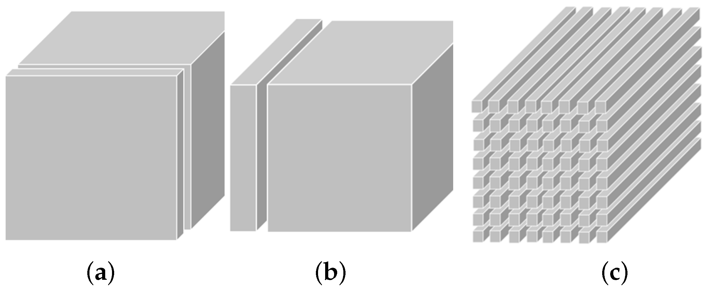
This section provides notations and definitions, offering a concise overview of relevant results that are subsequently applied in the ensuing discourse. Figure 1 illustrates the frontal slices (${\mathcal{A}}_{(:,:,k)}$), lateral slices (${\mathcal{A}}_{(:,j,:)}$), and tube fibers (${\mathcal{A}}_{(i,j,:)}$).

In this manuscript, we employ two operators, $\mathbf{unfold}$ and $\mathbf{fold}$. The operator $\mathbf{unfold}$ unfolds the tensor into a matrix of dimensions $ln\times m$, while $\mathbf{fold}$ serves as the inverse of $\mathbf{unfold}$ folding the matrix back into its original three-order tensor form. For clarity of exposition, we denote matrix $A_k$ specifically as the kth frontal slice of third-order tensor $\mathcal{A}\in {\mathbb{R}}^{l\times m\times n}$, i.e., $A_k={\mathcal{A}}_{(:,:,k)}$. We have  

$$\mathbf{unfold}\left(\mathcal{A}\right)=\left[\begin{array}{c}{A}_1\\ A_2\\ ⋮\\ A_n\end{array}\right],\mathbf{fold}\left(\mathbf{unfold}\left(\mathcal{A}\right)\right)=\mathcal{A}.$$

The forthcoming definitions and remarks, introduced herein, are utilized in the subsequent theoretical proofs.

Definition 1.

Assuming $\mathcal{A}$ is a third-order tensor, the block-circulant matrix $\mathbf{bcirc}\left(\mathcal{A}\right)$ is defined as follows:

$$\mathbf{bcirc}\left(\mathcal{A}\right)=\left[\begin{array}{cccc}\begin{array}{c}{A}_1\\ A_2\\ ⋮\\ A_n\end{array}& \begin{array}{c}{A}_n\\ A_1\\ ⋮\\ A_{n-1}\end{array}& \begin{array}{c}\cdots \\ \cdots \\ \ddots \\ \cdots \end{array}& \begin{array}{c}{A}_2\\ A_3\\ ⋮\\ A_1\end{array}\end{array}\right].$$

Definition 2

([9]). Given two tensors $\mathcal{A}\in {\mathbb{R}}^{l\times m\times n}$ and $\mathcal{B}\in {\mathbb{R}}^{m\times p\times n}$, the t-product $\mathcal{A}\ast \mathcal{B}$ is defined as

$$\mathcal{A}\ast \mathcal{B}=\mathbf{fold}\left(\mathbf{bcirc}\right(\mathcal{A}\left)\mathbf{unfold}\right(\mathcal{B}\left)\right)=\mathcal{C},$$

(10)

where $\mathcal{C}\in {\mathbb{R}}^{l\times p\times n}$.

Remark 1

([32]). For any two tensors $\mathcal{A}$ and $\mathcal{B}$ for which the t-product is defined, they satisfy

(1). $\mathbf{bcirc}(\mathcal{A}\ast \mathcal{B})=\mathbf{bcirc}\left(\mathcal{A}\right)\mathbf{bcirc}\left(\mathcal{B}\right)$.

(2). $\mathbf{bcirc}(\mathcal{A}+\mathcal{B})=\mathbf{bcirc}\left(\mathcal{A}\right)+\mathbf{bcirc}\left(\mathcal{B}\right)$.

(3). $\mathbf{bcirc}\left({\mathcal{A}}^T\right)=\mathbf{bcirc}{\left(\mathcal{A}\right)}^T$.

We define tensor $\widehat{\mathcal{A}}$ obtained by applying the Fast Fourier Transform (FFT) along each tube of $\mathcal{A}$, i.e.,

$$\mathbf{bdiag}\left(\widehat{\mathcal{A}}\right)=\left[\begin{array}{cccc}{\widehat{A}}_1& & & \\ & {\widehat{A}}_2& & \\ & & \ddots & \\ & & & {\widehat{A}}_n\end{array}\right]=\left(F_n\otimes I_l\right)\mathbf{bcirc}\left(\mathcal{A}\right)\left(F_n^{*}\otimes I_m\right),$$

(11)

where ⊗ is the Kronecker product, and matrix $F_n^{*}$ represents the conjugate transpose of the n-by-n unitary discrete Fourier transform matrix $F_n$. The structure of $F_n$ is defined as follows:

$$F_n=\frac{1}{\sqrt{n}}\left[\begin{array}{ccccc}1& 1& 1& \cdots & 1\\ 1& \omega & {\omega }^2& \cdots & {\omega }^{n-1}\\ 1& {\omega }^2& {\omega }^4& \cdots & {\omega }^{2\left(n-1\right)}\\ ⋮& ⋮& ⋮& \ddots & ⋮\\ 1& {\omega }^{n-1}& {\omega }^{2(n-1)}& \cdots & {\omega }^{\left(n-1\right)\left(n-1\right)}\end{array}\right],$$

where $\omega =e^{\frac{-2\pi i}{n}}$. Thus the t-product in (10) can be represented as

$$\mathcal{A}\ast \mathcal{B}=\mathbf{fold}\left(\left(F_n^{*}\otimes I_l\right)\left(\left(F_n\otimes I_l\right)\mathbf{bcirc}\left(\mathcal{A}\right)\left(F_n^{*}\otimes I_m\right)\right)\left(F_n\otimes I_m\right)\mathbf{unfold}\left(\mathcal{B}\right)\right),$$

(12)

and (10) is reformulated as

$$\left(\begin{array}{cccc}{\widehat{A}}_1& & & \\ & {\widehat{A}}_2& & \\ & & \ddots & \\ & & & {\widehat{A}}_n\end{array}\right)\left(\begin{array}{c}{\widehat{B}}_1\\ {\widehat{B}}_2\\ ⋮\\ {\widehat{B}}_n\end{array}\right)=\left(\begin{array}{c}{\widehat{C}}_1\\ {\widehat{C}}_2\\ ⋮\\ {\widehat{C}}_n\end{array}\right).$$

(13)

It is easy to calculate (12) in MATLAB.

For a non-zero tensor $\overrightarrow{\mathcal{X}}\in {\mathbb{R}}^{m\times 1\times n}$, we can decompose it in the form

$$\overrightarrow{\mathcal{X}}=\overrightarrow{\mathcal{D}}\ast \mathit{d},$$

(14)

where $\overrightarrow{\mathcal{D}}\in {\mathbb{R}}^{m\times 1\times n}$ is a normalized tensor; see, e.g., ref. [11], and $d\in {\mathbb{R}}^{1\times 1\times n}$ is a tube scalar. Algorithm 1 summarizes the decomposition in (14).

Algorithm 1 Normalization

Input:$\overrightarrow{\mathcal{X}}\in {\mathbb{R}}^{m\times 1\times n}$ is a nonzero tensor Output:$\overrightarrow{\mathcal{D}}$, $\mathit{d}$ with $\overrightarrow{\mathcal{X}}=\overrightarrow{\mathcal{D}}\ast \mathit{d}$, $\parallel \overrightarrow{\mathcal{D}}\parallel =1$ $\overrightarrow{\mathcal{D}}\leftarrow$ fft($\overrightarrow{\mathcal{X}}$,[ ],3) for  $j=1,2,\dots ,n$  do     ${\mathit{d}}_j\leftarrow {\parallel \overrightarrow{{\mathcal{D}}_j}\parallel }_2$ (${\overrightarrow{\mathcal{D}}}_j$ is a vector)     if ${\mathit{d}}_j>tol$ then         $\overrightarrow{{\mathcal{D}}_j}\leftarrow \frac{1}{{\mathit{d}}_j}{\overrightarrow{\mathcal{D}}}_j$     else         ${\overrightarrow{\mathcal{D}}}_j\leftarrow \mathbf{randn}(m,1)$; ${\mathit{d}}_j\leftarrow {\parallel \overrightarrow{{\mathcal{D}}_j}\parallel }_2$; $\overrightarrow{{\mathcal{D}}_j}\leftarrow \frac{1}{{\mathit{d}}_j}{\overrightarrow{\mathcal{D}}}_j$; ${\mathit{d}}_j\leftarrow 0$     end if end for $\overrightarrow{\mathcal{D}}\leftarrow$ ifft($\overrightarrow{\mathcal{D}}$,[ ],3); $\mathit{d}\leftarrow$ ifft($\mathit{d}$,[ ],3)

Given tensor $\mathcal{A}\in {\mathbb{R}}^{l\times m\times n}$, the singular value decomposition (tSVD) of $\mathcal{A}$ is expressed as

$$\mathcal{A}=\mathcal{U}\ast \mathcal{S}\ast {\mathcal{V}}^T,$$

where $\mathcal{U}\in {\mathbb{R}}^{l\times l\times n}$ and $\mathcal{V}\in {\mathbb{R}}^{m\times m\times n}$ are orthogonal under the t-product;

$$\mathcal{S}=\mathrm{diag}[s_1,s_2,\dots ,s_{min\{l,m\}}]\in {\mathbb{R}}^{m\times l\times n}$$

is an upper triangular tensor with the singular tubes $s_j$ satisfying

$${\parallel s_1\parallel }_F\ge {\parallel s_2\parallel }_F\ge \cdots \ge {\parallel s_{min\left\{l,m\right\}}\parallel }_F.$$

Algorithm 2 introduces the tensor Conjugate Gradient (t-CG) method, presented in [11], for solving the least squares solution of the tensor linear systems (1).

Algorithm 2 The tCG method for sloving (4).

Input:  $\mathcal{A}\in {\mathbb{R}}^{m\times m\times n},\overrightarrow{\mathcal{B}}\in {\mathbb{R}}^{m\times 1\times n}$, $\mu$. Output: Approximate solution ${\overrightarrow{\mathcal{X}}}^{*}$ of Problem (4). ${\overrightarrow{\mathcal{X}}}_0=0,k=0$. $[{\overrightarrow{\mathcal{R}}}_0,a]\leftarrow$ Normalize$({\mathcal{A}}^T\ast \overrightarrow{\mathcal{B}}-({\mathcal{A}}^T\ast \mathcal{A}+\mu \mathcal{I})\ast {\overrightarrow{\mathcal{X}}}_0)$; ${\overrightarrow{\mathcal{P}}}_0\leftarrow {\overrightarrow{\mathcal{R}}}_0$. for $i=1,2,\dots$ until $\sigma <tol$ do     $c={\left({\overrightarrow{\mathcal{P}}}_{i-1}^T\ast ({\mathcal{A}}^T\ast \mathcal{A}+\mu \mathcal{I})\ast {\overrightarrow{\mathcal{P}}}_{i-1}\right)}^{-1}\ast \left({\overrightarrow{\mathcal{R}}}_{i-1}^T\ast {\overrightarrow{\mathcal{R}}}_{i-1}\right)$.     ${\overrightarrow{\mathcal{X}}}_i={\overrightarrow{\mathcal{X}}}_{i-1}+{\overrightarrow{\mathcal{P}}}_{i-1}\ast c$.     ${\overrightarrow{\mathcal{R}}}_i={\overrightarrow{\mathcal{R}}}_{i-1}-({\mathcal{A}}^T\ast \mathcal{A}+{\mu }_k\mathcal{I})\ast \left({\overrightarrow{\mathcal{P}}}_{i+1}\ast c\right).$     $\sigma =|{\parallel {\overrightarrow{\mathcal{R}}}_i\parallel }_F-{\parallel {\overrightarrow{\mathcal{R}}}_{i-1}\parallel }_F|.$     $d={\left({\overrightarrow{\mathcal{R}}}_{i-1}^T\ast {\overrightarrow{\mathcal{R}}}_{i-1}\right)}^{-1}\ast \left({\overrightarrow{\mathcal{R}}}_i^T\ast {\overrightarrow{\mathcal{R}}}_i\right)$.     ${\overrightarrow{\mathcal{P}}}_i={\overrightarrow{\mathcal{R}}}_i+{\overrightarrow{\mathcal{P}}}_{i-1}\ast d$. end for ${\overrightarrow{\mathcal{X}}}^{*}={\overrightarrow{\mathcal{X}}}_i\ast a$

The operators $\mathbf{squeeze}$ and $\mathbf{twist}$ [11] are expressed by

$$X=\mathbf{squeeze}\left({\overrightarrow{\mathcal{X}}}_j\right)⟹X(i,j)={\overrightarrow{\mathcal{X}}}_{(i,1,j)},\mathbf{twist}\left(\mathbf{squeeze}\left(\overrightarrow{\mathcal{X}}\right)\right)=\overrightarrow{\mathcal{X}}.$$

Figure 2 illustrates the transformation between a matrix and a tensor column by using $\mathbf{squeeze}$ and $\mathbf{twist}$. Generally, operators ${\mathbf{multi}}_{-}\mathbf{squeeze}$ and ${\mathbf{multi}}_{-}\mathbf{twist}$ are defined for a third-order tensor to make it squeezed or twisted. For tensor $\mathcal{D}\in {\mathbb{R}}^{m\times p\times n}$ with $p>1$, $\mathcal{C}={\mathbf{multi}}_{-}\mathbf{squeeze}\left(\mathcal{D}\right)$ means that all side slices of $\mathcal{D}$ are squeezed and stacked as front slices of $\mathcal{C}$, the operator ${\mathbf{multi}}_{-}\mathbf{twist}$ is the reverse operation of ${\mathbf{multi}}_{-}\mathbf{squeeze}$. Thus, ${\mathbf{multi}}_{-}\mathbf{twist}\left({\mathbf{multi}}_{-}\mathbf{squeeze}\left(\mathcal{D}\right)\right)=\mathcal{D}$. We refer to

Table 1. Notation Explanation.

Notation	Interpretation
A	matrix
I	identity matrix
${\mathcal{A}}^T$	transpose of tensor
${\mathcal{A}}^{-1}$	inverse of tensor, ${\mathcal{A}}^{-T}={\left({\mathcal{A}}^{-1}\right)}^T={\left({\mathcal{A}}^T\right)}^{-1}$
$\widehat{\mathcal{A}}$	FFT of $\mathcal{A}$ along the third mode
$\mathcal{I}$	identity tensor
${\parallel \mathcal{A}\parallel }_F$	the Frobenius norm, i.e, ${\parallel \mathcal{A}\parallel }_F=\sqrt{{\sum }_{i=1}^l{\sum }_{j=1}^m{\sum }_{k=1}^n{a}_{ijk}^2}.$
∗	t-product
${\overrightarrow{\mathcal{A}}}_j$, ${\mathcal{A}}_{(:,j,:)}$	the jth tensor column of $\mathcal{A}$, jth lateral slice of $\mathcal{A}$
${\mathcal{A}}_{(:,:,k)}$	the kth frontal slice of tensor $\mathcal{A}$
$\mathit{d}$	tube
$〈\mathcal{A},\mathcal{B}〉$	$〈\mathcal{A},\mathcal{B}〉={\sum }_{ijk}{a}_{ijk}{b}_{ijk}$
$〈\overrightarrow{\mathcal{A}},\overrightarrow{\mathcal{B}}〉$	$〈\overrightarrow{\mathcal{A}},\overrightarrow{\mathcal{B}}〉={\sum }_{ik}{a}_{i1k}{b}_{i1k}$

for more notations and definitions.

3. Tensor Conjugate Gradient Methods

This section initiates the discussion on the automated determination of an appropriate regularization parameter for the tensor Conjugate Gradient (tCG) method. We abbreviate the improved method as auto-tCG. A truncated auto-tCG method is developed to improve the auto-tCG method and is abbreviated as auto-ttCG. A  preprocessed version of the auto-ttCG method is presented, which is abbreviated as auto-ttpCG.

3.1. The Auto-tCG Method

The regularization parameter in the t-CG method was not discussed and was user-specified. This subsection enhances the t-CG method by utilizing the discrepancy principle for the determination of an appropriate regularization parameter, operating under the assumption (3) and uses it to solve the normal Equation (6). We consider the polynomial function

$${\mu }_k={\mu }_0{q}^k,k=0,1,\dots ,$$

(15)

where $q\in (0,1)$. We set ${\mu }_0={\parallel \mathcal{A}\parallel }_F$ and obtain an optimal regularization parameter by continuously reducing the parameter. An effective method to deal with general Problems (9) is to regard it as p independent subproblems (4), i.e.,  

$$\underset{{\overrightarrow{\mathcal{X}}}_j\in {\mathbb{R}}^{m\times 1\times n}}{min}\left\{{\parallel \mathcal{A}\ast {\overrightarrow{\mathcal{X}}}_j-{\overrightarrow{\mathcal{B}}}_j\parallel }_F^2+\mu {\parallel {\overrightarrow{\mathcal{X}}}_j\parallel }_F^2\right\},j=1,\dots ,p,$$

(16)

where ${\overrightarrow{\mathcal{B}}}_j$ is the tensor column of tensor $\mathcal{B}$ and is polluted by noise $\overrightarrow{{\mathcal{E}}_j}$. ${\overrightarrow{\mathcal{B}}}_{j,true}$ represents unknown error-free tensor. We assume noise tensor

$$\overrightarrow{{\mathcal{E}}_j}=\overrightarrow{{\mathcal{B}}_j}-{\overrightarrow{\mathcal{B}}}_{j,true}$$

can be used or the norm of ${\overrightarrow{\mathcal{E}}}_j$ can be estimated, i.e.,

$${\parallel {\overrightarrow{\mathcal{E}}}_j\parallel }_F\le {\delta }_j,j=1,\dots ,p.$$

Algorithm 3 encapsulates the auto-tCG method designed for solving Equation (9). The initial tensor of Algorithm 3 is set as a zero tensor. The iteration concludes when the Frobenius norm of the residual tensor

$${\overrightarrow{\mathcal{R}}}_{j,{\mu }_k}^i={\mathcal{A}}^T\ast {\overrightarrow{\mathcal{B}}}_j-({\mathcal{A}}^T\ast \mathcal{A}+{\mu }_k\mathcal{I})\ast {\overrightarrow{\mathcal{X}}}_{j,{\mu }_k}^i$$

is small enough, where ${\overrightarrow{\mathcal{R}}}_{j,{\mu }_k}^i$ denotes the residual generated by the ith iterative solution ${\overrightarrow{\mathcal{X}}}_{j,{\mu }_k}^i$ of the normal equation with ${\mu }_k$ of the jth independent subproblem. We let ${\overrightarrow{\mathcal{X}}}_{int}={\overrightarrow{\mathcal{X}}}_{{\mu }_k}^{*}$ be the initial tensor of the normal equation of ${\mu }_{k+1}$. When $\mu ={\mu }_k$ with m iterations for the CG-process, the affine space is ${\overrightarrow{\mathcal{X}}}_{{\mu }_k}^0+{\mathcal{K}}_m\left({\mathcal{A}}^T\ast \mathcal{A}+{\mu }_k\mathcal{I},r_{{\mu }_k}^0\right)$, where $r_{{\mu }_k}^0={\mathcal{A}}^T\ast \overrightarrow{\mathcal{B}}-\left({\mathcal{A}}^T\ast \mathcal{A}+{\mu }_k\mathcal{I}\right)\ast {\overrightarrow{\mathcal{X}}}_{{\mu }_k}^0$.

Algorithm 3 The auto-tCG method for sloving (9).

Input: $\mathcal{A}\in {\mathbb{R}}^{m\times m\times n},\overrightarrow{{\mathcal{B}}_j}\in {\mathbb{R}}^{m\times 1\times n}$, ${\delta }_j$, $j=1,\dots ,p$, ${\mu }_0$, $\eta >1$. Output: Approximate solution ${\mathcal{X}}^{*}$ of Problem (9). for  $j=1,2,\dots p$  do     ${\overrightarrow{\mathcal{X}}}_{int}=0,k=0$.     while $\mathbf{do}{\parallel \mathcal{A}\ast {\overrightarrow{\mathcal{X}}}_{j,{\mu }_k}^{*}-{\overrightarrow{\mathcal{B}}}_j\parallel }_F^2>{\eta }^2{\delta }_j^2$         $k=k+1$, $({\mathcal{A}}^T\ast \mathcal{A}+{\mu }_k\mathcal{I})\ast {\overrightarrow{\mathcal{X}}}_j={\mathcal{A}}^T\ast {\overrightarrow{\mathcal{B}}}_j$, e.g., ${\mu }_k={\mu }_0{q}^k$         $[{\overrightarrow{\mathcal{R}}}_0,a]\leftarrow$ Normalize$({\mathcal{A}}^T\ast {\overrightarrow{\mathcal{B}}}_j-({\mathcal{A}}^T\ast \mathcal{A}+{\mu }_k\mathcal{I})\ast {\overrightarrow{\mathcal{X}}}_{int})$; ${\overrightarrow{\mathcal{P}}}_0\leftarrow {\overrightarrow{\mathcal{R}}}_0$.         $i=0$, $\sigma >tol$.         while $\sigma >tol$ do            $i=i+1$.            $c={\left({\overrightarrow{\mathcal{P}}}_{i-1}^T\ast ({\mathcal{A}}^T\ast \mathcal{A}+{\mu }_k\mathcal{I})\ast {\overrightarrow{\mathcal{P}}}_{i-1}\right)}^{-1}\ast \left({\overrightarrow{\mathcal{R}}}_{i-1}^T\ast {\overrightarrow{\mathcal{R}}}_{i-1}\right)$.            ${\overrightarrow{\mathcal{X}}}_i={\overrightarrow{\mathcal{X}}}_{i-1}+{\overrightarrow{\mathcal{P}}}_{i-1}\ast c$.            ${\overrightarrow{\mathcal{R}}}_i={\overrightarrow{\mathcal{R}}}_{i-1}-({\mathcal{A}}^T\ast \mathcal{A}+{\mu }_k\mathcal{I})\ast \left({\overrightarrow{\mathcal{P}}}_{i+1}\ast c\right).$            $\sigma =|{\parallel {\overrightarrow{\mathcal{R}}}_i\parallel }_F-{\parallel {\overrightarrow{\mathcal{R}}}_{i-1}\parallel }_F|.$            $d={\left({\overrightarrow{\mathcal{R}}}_{i-1}^T\ast {\overrightarrow{\mathcal{R}}}_{i-1}\right)}^{-1}\ast \left({\overrightarrow{\mathcal{R}}}_i^T\ast {\overrightarrow{\mathcal{R}}}_i\right)$.            ${\overrightarrow{\mathcal{P}}}_i={\overrightarrow{\mathcal{R}}}_i+{\overrightarrow{\mathcal{P}}}_{i-1}\ast d$.         end while         ${\overrightarrow{\mathcal{X}}}_{j,{\mu }_k}^{*}={\overrightarrow{\mathcal{X}}}_i\ast a$ (${\overrightarrow{\mathcal{X}}}_{j,{\mu }_k}^{*}$ is the solution of the normal equation about ${\mu }_k$ of the jth independent Subproblem (4)).         ${\overrightarrow{\mathcal{X}}}_{int}={\overrightarrow{\mathcal{X}}}_{j,{\mu }_k}^{*}.$     end while     ${\mathcal{X}}_{(:,j,:)}^{*}={\overrightarrow{\mathcal{X}}}_{j,{\mu }_k}^{*}$. end for

3.2. The Truncated Tensor Conjugate Gradient Method

Frommer and Maass in [33] proposed a good condition that can roughly judge some inappropriate value of $\mu$. We introduce this condition to improve Algorithm 3 by excluding some unsuitable value of $\mu$, and present a truncated tensor Conjugate Gradient method for solving (9). We first provide the following results:

Theorem 1.

Given $\mathcal{A}\in {\mathbb{R}}^{l\times m\times n}$, we define a t-linear operator T: ${\mathbb{R}}^{m\times 1\times n}\to {\mathbb{R}}^{l\times 1\times n}$, i.e.,  $T\left(\overrightarrow{\mathcal{X}}\right)=\mathcal{A}\ast \overrightarrow{\mathcal{X}}$ with $\overrightarrow{\mathcal{X}}\in {\mathbb{R}}^{m\times 1\times n}$. We let ${\overrightarrow{\mathcal{X}}}_{\mu }^{*}$ be the exact solution of the normal equations

$$({\mathcal{A}}^T\ast \mathcal{A}+\mu \mathcal{I})\ast \overrightarrow{\mathcal{X}}={\mathcal{A}}^T\ast \overrightarrow{\mathcal{B}};$$

then, for an arbitrary $\mathcal{X}\in {\mathbb{R}}^{m\times 1\times n}$, we have

$${\parallel \mathcal{A}\ast {\overrightarrow{\mathcal{X}}}_{\mu }^{*}-\overrightarrow{\mathcal{B}}\parallel }_F^2\ge {\parallel \mathcal{A}\ast \overrightarrow{\mathcal{X}}-\overrightarrow{\mathcal{B}}\parallel }_F^2-\frac{1}{4\mu }{\parallel {\mathcal{A}}^T\ast \overrightarrow{\mathcal{B}}-({\mathcal{A}}^T\ast \mathcal{A}+\mu \mathcal{I})\ast \overrightarrow{\mathcal{X}}\parallel }_F^2.$$

Proof. 

For an arbitrary $\overrightarrow{\mathcal{X}}\in {\mathbb{R}}^{m\times 1\times n}$, we set $\overrightarrow{\mathcal{Z}}={\overrightarrow{\mathcal{X}}}_{\mu }^{*}-\overrightarrow{\mathcal{X}}$. We let the singular value decomposition of $\mathcal{A}$ be $\mathcal{A}=\mathcal{U}\ast \mathcal{S}\ast {\mathcal{V}}^T$; then,

$$\mathcal{A}\ast \overrightarrow{\mathcal{Z}}=\mathcal{U}\ast \mathcal{S}\ast {\mathcal{V}}^T\ast \overrightarrow{\mathcal{Z}}.$$

We suppose ${\mathcal{V}}^T\ast \overrightarrow{\mathcal{Z}}=\overrightarrow{\mathcal{D}}\in {\mathbb{R}}^{m\times 1\times n}$; then,

$${\parallel \mathcal{A}\ast \overrightarrow{\mathcal{Z}}\parallel }_F^2={\parallel \mathcal{U}\ast \mathcal{S}\ast {\mathcal{V}}^T\ast \overrightarrow{\mathcal{Z}}\parallel }_F^2={\parallel \mathcal{S}\ast \overrightarrow{\mathcal{D}}\parallel }_F^2={\parallel \mathbf{bcirc}\left(\mathcal{S}\right)\mathbf{unfold}\left(\overrightarrow{\mathcal{D}}\right)\parallel }_2^2.$$

(17)

Thus,

$$\begin{array}{cc}\hfill & {\parallel ({\mathcal{A}}^T\ast \mathcal{A}+\mu \mathcal{I})\ast \overrightarrow{\mathcal{Z}}\parallel }_F^2\hfill \\ \hfill =& {\parallel \mathcal{V}\ast ({\mathcal{S}}^T\ast \mathcal{S}+\mu \mathcal{I})\ast {\mathcal{V}}^T\ast \overrightarrow{\mathcal{Z}}\parallel }_F^2={\parallel \mathcal{V}\ast ({\mathcal{S}}^T\ast \mathcal{S}+\mu \mathcal{I})\ast \overrightarrow{\mathcal{D}}\parallel }_F^2\hfill \\ \hfill =& {\parallel \left({\mathcal{S}}^T\ast \mathcal{S}+\mu \mathcal{I}\right)\ast \overrightarrow{\mathcal{D}}\parallel }_F^2={\parallel (\mathbf{bcirc}({\mathcal{S}}^T\ast \mathcal{S})+\mu \mathbf{bcirc}\left(\mathcal{I}\right))\mathbf{unfold}\left(\overrightarrow{\mathcal{D}}\right)\parallel }_2^2\hfill \\ \hfill =& {\parallel (\mathbf{bcirc}{\left(\mathcal{S}\right)}^T\mathbf{bcirc}\left(\mathcal{S}\right)+\mu \mathbf{bcirc}\left(\mathcal{I}\right))\mathbf{unfold}\left(\overrightarrow{\mathcal{D}}\right)\parallel }_2^2.\hfill \end{array}$$

(18)

We denote $\mathbf{bcirc}\left(\mathcal{S}\right)=\mathbf{S}\in {\mathbb{R}}^{nl\times nm}$, $\mathbf{bcirc}\left(\mathcal{I}\right)=\mathbf{I}\in {\mathbb{R}}^{nm\times nm}$ and $\mathbf{unfold}\left(\overrightarrow{\mathcal{D}}\right)=\mathbf{d}\in {\mathbb{R}}^{nm\times 1}$, then ${\parallel \mathcal{A}\ast \overrightarrow{\mathcal{Z}}\parallel }_F^2={\parallel \mathbf{S}\mathbf{d}\parallel }_2^2$ and ${\parallel ({\mathcal{A}}^T\ast \mathcal{A}+\mu \mathcal{I})\ast \overrightarrow{\mathcal{Z}}\parallel }_F^2={\parallel ({\mathbf{S}}^T\mathbf{S}+\mu \mathbf{I})\mathbf{d}\parallel }_2^2$. Thus, we transform the tensor norm into the equivalent matrix norm. We let the singular value decomposition of $\mathbf{S}$ be $\mathbf{S}=\mathbf{U}\Sigma {\mathbf{V}}^T$, where $\Sigma =\mathrm{diag}\left({\sigma }_1,{\sigma }_2,\dots ,{\sigma }_r\right),r\le min\left\{nl,nm\right\}$, $\mathbf{U}=[{\mathbf{u}}_1,{\mathbf{u}}_2,\dots ,{\mathbf{u}}_r]$ and $\mathbf{V}=[{\mathbf{v}}_1,{\mathbf{v}}_2,\dots ,{\mathbf{v}}_r]$ are orthogonal matrices with orthogonal columns ${\mathbf{u}}_k\in {\mathbb{R}}^{nl\times 1}$ and ${\mathbf{v}}_k\in {\mathbb{R}}^{nm\times 1}$, respectively. Thus, we have

$$\mathbf{S}\mathbf{d}=\sum _{{\sigma }_k>0}{\sigma }_k〈\mathbf{d},{\mathbf{v}}_k〉{\mathbf{u}}_k.$$

Using equation $s^2={(s+\mu s^{-1})}^{-2}{(s^2+\mu )}^2$ with estimate

$$\frac{1}{s+\mu s^{-1}}\le \frac{1}{2\sqrt{\mu }},(s,\mu >0),$$

we have

$$\begin{array}{cc}\hfill {\parallel \mathbf{Sd}\parallel }_2^2& =\sum _{{\sigma }_k>0}{{\sigma }_k^2\left|〈\mathbf{d},v_k〉\right|}^2=\sum _{{\sigma }_k>0}{\left({\sigma }_k+\mu {\sigma }_k^{-1}\right)}^{-2}{\left({\sigma }_k^2+\mu \right)}^2{\left|〈\mathbf{d},v_k〉\right|}^2\hfill \\ \hfill & \le \frac{1}{4\mu }\sum _{{\sigma }_k>0}{\left({\sigma }_k^2+\mu \right)}^2{\left|〈\mathbf{d},v_k〉\right|}^2.\hfill \end{array}$$

(19)

We note that

$${\parallel \left({\mathbf{S}}^T\mathbf{S}+\mu \mathbf{I}\right)\mathbf{d}\parallel }_2^2=\sum _{{\sigma }_k>0}{{\left({\sigma }_k^2+\mu \right)}^2\left|〈\mathbf{d},v_k〉\right|}^2.$$

(20)

It results from (19) and (20) that

$${\parallel \mathbf{Sd}\parallel }_2^2\le \frac{1}{4\mu }{\parallel \left({\mathbf{S}}^T\mathbf{S}+\mu \mathbf{I}\right)\mathbf{d}\parallel }_2^2.$$

We note that ${\parallel \mathcal{A}\ast \overrightarrow{\mathcal{Z}}\parallel }_F^2={\parallel \mathbf{S}\mathbf{d}\parallel }_2^2$ and ${\parallel ({\mathcal{A}}^T\ast \mathcal{A}+\mu \mathcal{I})\ast \overrightarrow{\mathcal{Z}}\parallel }_F^2={\parallel ({\mathbf{S}}^T\mathbf{S}+\mu \mathbf{I})\mathbf{d}\parallel }_2^2$; we have

$${\parallel \mathcal{A}\ast \overrightarrow{\mathcal{Z}}\parallel }_F^2\le \frac{1}{4\mu }{\parallel ({\mathcal{A}}^T\ast \mathcal{A}+\mu \mathcal{I})\ast \overrightarrow{\mathcal{Z}}\parallel }_F^2.$$

(21)

Thus,

$$\begin{array}{cc}\hfill {\parallel \mathcal{A}\ast {\overrightarrow{\mathcal{X}}}_{\mu }^{\ast }-\overrightarrow{\mathcal{B}}\parallel }_F^2& ={\parallel \mathcal{A}\ast \overrightarrow{\mathcal{X}}-\overrightarrow{\mathcal{B}}+\mathcal{A}\ast \left({\overrightarrow{\mathcal{X}}}_{\mu }^{\ast }-\overrightarrow{\mathcal{X}}\right)\parallel }_F^2\hfill \\ \hfill & \ge {\parallel \mathcal{A}\ast \overrightarrow{\mathcal{X}}-\overrightarrow{\mathcal{B}}\parallel }_F^2-{\parallel \mathcal{A}\ast \overrightarrow{\mathcal{Z}}\parallel }_F^2\hfill \\ \hfill & \ge {\parallel \mathcal{A}\ast \overrightarrow{\mathcal{X}}-\overrightarrow{\mathcal{B}}\parallel }_F^2-\frac{1}{4\mu }{\parallel \left({\mathcal{A}}^T\ast \mathcal{A}+\mu \overrightarrow{\mathcal{I}}\right)\overrightarrow{\mathcal{Z}}\parallel }_F^2.\hfill \end{array}$$

(22)

We note that

$$\begin{array}{cc}\hfill ({\mathcal{A}}^T\ast \mathcal{A}+\mu \mathcal{I})\ast \overrightarrow{\mathcal{Z}}& =({\mathcal{A}}^T\ast \mathcal{A}+\mu \mathcal{I})\ast ({\overrightarrow{\mathcal{X}}}_{\mu }^{*}-\overrightarrow{\mathcal{X}})={\mathcal{A}}^T\ast \overrightarrow{\mathcal{B}}-({\mathcal{A}}^T\ast \mathcal{A}+\mu \mathcal{I})\ast \overrightarrow{\mathcal{X}};\hfill \end{array}$$

(23)

then, (23) and (22) result in

$${\parallel \mathcal{A}\ast {\overrightarrow{\mathcal{X}}}_{\mu }^{*}-\overrightarrow{\mathcal{B}}\parallel }_F^2\ge {\parallel \mathcal{A}\ast \overrightarrow{\mathcal{X}}-\overrightarrow{\mathcal{B}}\parallel }_F^2-\frac{1}{4\mu }{\parallel {\mathcal{A}}^T\ast \overrightarrow{\mathcal{B}}-({\mathcal{A}}^T\ast \mathcal{A}+\mu \mathcal{I})\ast \overrightarrow{\mathcal{X}}\parallel }_F^2.$$

   □

We apply Theorem 1 to predict in advance whether the exact solution ${\overrightarrow{\mathcal{X}}}_{{\mu }_k}^{*}$ satisfies the discrepancy principle in Algorithm 3. We add condition

$${\parallel \mathcal{A}\ast {\overrightarrow{\mathcal{X}}}_{{\mu }_k}^i-\overrightarrow{\mathcal{B}}\parallel }_F^2-\frac{1}{4{\mu }_k}{\parallel {\overrightarrow{\mathcal{R}}}_{{\mu }_k}^i\parallel }_F^2>{\eta }^2{\delta }^2$$

(24)

in Steps 9–16 of Algorithm 3. If the ith iteration solution of the normal equation with ${\mu }_k$ is ${\overrightarrow{\mathcal{X}}}_{{\mu }_k}^i$ and its residual ${\overrightarrow{\mathcal{R}}}_{{\mu }_k}^i$ satisfies (24), then ${\parallel \mathcal{A}\ast {\overrightarrow{\mathcal{X}}}_{{\mu }_k}^{*}-\overrightarrow{\mathcal{B}}\parallel }_F^2>{\eta }^2{\delta }^2$. This indicates that the exact solution of the normal equation with ${\mu }_k$ does not satisfy the discrepancy principle, so we continue to solve next normal equation with ${\mu }_{k+1}$. Therefore, we obtain a truncated tensor Conjugate Gradient method of automatical determination of a suitable regularization parameter, which is abbreviated as auto-ttCG. Algorithm 4 summarizes the auto-ttCG method.

3.3. A Preconditioned Truncated Tensor Conjugate Gradient Method

In this section, we explore the acceleration of Algorithm 4 through preconditioning. When tensor $\mathcal{M}$ is symmetric positive definite under the t-product structure, we can obtain its tensor approximate Cholesky decomposition (tChol) by Algorithm 5.

In Algorithm 4, coefficient tensor ${\mathcal{A}}^T\ast \mathcal{A}+{\mu }_k\mathcal{I}$ of kth normal equation

$$({\mathcal{A}}^T\ast \mathcal{A}+{\mu }_k\mathcal{I})\ast \overrightarrow{\mathcal{X}}={\mathcal{A}}^T\ast \overrightarrow{\mathcal{B}}$$

(25)

is symmetric and positive definite. We set $\mathcal{M}={\mathcal{A}}^T\ast \mathcal{A}+{\mu }_k\mathcal{I}$ and apply Algorithm 5 to obtain the decomposition of $\mathcal{M}=\mathcal{H}\ast {\mathcal{H}}^T$, where each frontal slice of $\mathcal{H}$ is a fully sparse lower triangular matrix. After normal Equation (25) is preconditioned by $\mathcal{M}$, we solve preconditioned normal equations

$$\tilde{\mathcal{A}}\ast \widetilde{\overrightarrow{\mathcal{X}}}=\widetilde{\overrightarrow{\mathcal{B}}}$$

(26)

instead of Equation (25) in Algorithm 4, where $\tilde{\mathcal{A}}={\mathcal{H}}^{-1}\ast ({\mathcal{A}}^T\ast \mathcal{A}+{\mu }_k\mathcal{I})\ast {\mathcal{H}}^{-T}$, $\widetilde{\overrightarrow{\mathcal{X}}}={\mathcal{H}}^T\ast \overrightarrow{\mathcal{X}}$, $\widetilde{\overrightarrow{\mathcal{B}}}={\mathcal{H}}^{-1}\ast {\mathcal{A}}^T\ast \overrightarrow{\mathcal{B}}$.

Algorithm 4 The auto-ttCG method for sloving (9)

Input: $\mathcal{A}\in {\mathbb{R}}^{m\times m\times n},\overrightarrow{{\mathcal{B}}_j}\in {\mathbb{R}}^{m\times 1\times n}$, ${\delta }_j$, $j=1,\dots ,p$, ${\mu }_0$, $\eta >1$, tol. Output: Approximate solution ${\mathcal{X}}^{*}$ of Problem (9). for  $j=1,2,\dots p$  do     ${\overrightarrow{\mathcal{X}}}_{int}=0,k=0$     while ${\parallel \mathcal{A}\ast {\overrightarrow{\mathcal{X}}}_{j,{\mu }_k}^i-{\overrightarrow{\mathcal{B}}}_j\parallel }_F^2>{\eta }^2{\delta }_j^2$ do         $k=k+1$, $({\mathcal{A}}^T\ast \mathcal{A}+{\mu }_k\mathcal{I})\ast {\overrightarrow{\mathcal{X}}}_j={\mathcal{A}}^T\ast {\overrightarrow{\mathcal{B}}}_j$, e.g., ${\mu }_k={\mu }_0{q}^k$.         $[{\overrightarrow{\mathcal{R}}}_0,a]\leftarrow$ Normalize$({\mathcal{A}}^T\ast {\overrightarrow{\mathcal{B}}}_j-({\mathcal{A}}^T\ast \mathcal{A}+{\mu }_k\mathcal{I})\ast {\overrightarrow{\mathcal{X}}}_{int})$; ${\overrightarrow{\mathcal{P}}}_0\leftarrow {\overrightarrow{\mathcal{R}}}_0$.         $i=0$, $\sigma$ = 10 tol, ${\overrightarrow{\mathcal{X}}}_{j,{\mu }_k}^0={\overrightarrow{\mathcal{X}}}_{int}$.         while $\sigma >tol$ and ${\parallel \mathcal{A}\ast {\overrightarrow{\mathcal{X}}}_{j,{\mu }_k}^i-\overrightarrow{\mathcal{B}}\parallel }_F^2-\frac{1}{4{\mu }_k}{\parallel {\overrightarrow{\mathcal{R}}}_i\ast a\parallel }_F^2<{\eta }^2{\delta }^2$ do            $i=i+1$.            $c={\left({\overrightarrow{\mathcal{P}}}_{i-1}^T\ast ({\mathcal{A}}^T\ast \mathcal{A}+{\mu }_k\mathcal{I})\ast {\overrightarrow{\mathcal{P}}}_{i-1}\right)}^{-1}\ast \left({\overrightarrow{\mathcal{R}}}_{i-1}^T\ast {\overrightarrow{\mathcal{R}}}_{i-1}\right)$.            ${\overrightarrow{\mathcal{X}}}_i={\overrightarrow{\mathcal{X}}}_{i-1}+{\overrightarrow{\mathcal{P}}}_{i-1}\ast c$, ${\overrightarrow{\mathcal{X}}}_{j,{\mu }_k}^i={\overrightarrow{\mathcal{X}}}_i\ast a$.            ${\overrightarrow{\mathcal{R}}}_i={\overrightarrow{\mathcal{R}}}_{i-1}-({\mathcal{A}}^T\ast \mathcal{A}+{\mu }_k\mathcal{I})\ast \left({\overrightarrow{\mathcal{P}}}_{i+1}\ast c\right)$            $\sigma =|{\parallel {\overrightarrow{\mathcal{R}}}_i\parallel }_F-{\parallel {\overrightarrow{\mathcal{R}}}_{i-1}\parallel }_F|$.            $d={\left({\overrightarrow{\mathcal{R}}}_{i-1}^T\ast {\overrightarrow{\mathcal{R}}}_{i-1}\right)}^{-1}\ast \left({\overrightarrow{\mathcal{R}}}_i^T\ast {\overrightarrow{\mathcal{R}}}_i\right)$.            ${\overrightarrow{\mathcal{P}}}_i={\overrightarrow{\mathcal{R}}}_i+{\overrightarrow{\mathcal{P}}}_{i-1}\ast d$.         end while         ${\overrightarrow{\mathcal{X}}}_{int}={\overrightarrow{\mathcal{X}}}_{{\mu }_k}^i$.     end while     ${\mathcal{X}}_{(:,j,:)}^{\ast }={\overrightarrow{\mathcal{X}}}_{j,{\mu }_k}^i$. end for

Algorithm 5 Tensor Cholesky decomposition (tChol)

1: Input:  $\mathcal{M}\in {\mathbb{R}}^{m\times m\times n}\ne \mathcal{O}$ 2: Output: $\mathcal{H}\in {\mathbb{R}}^{m\times m\times n}$ and $\mathcal{M}=\mathcal{H}\ast {\mathcal{H}}^T$. 3: $\widehat{\mathcal{M}}\leftarrow$ fft($\mathcal{M}$,[ ],3) 4: for  $j=1,2,\dots ,n$  do 5:     $H\leftarrow chol\left({\widehat{\mathcal{M}}}_{(:,:,j)}\right)$, H is the lower triangular matrix, which is obtained by approximate Cholesky decomposition. 6:     ${\widehat{\mathcal{H}}}_{\left(:,:,j\right)}\leftarrow H$. 7: end for 8: $\mathcal{H}\leftarrow$ ifft($\widehat{\mathcal{H}}$,[ ],3).

We apply Algorithm 4 to solve (26) instead of (25). We let ${\overrightarrow{\mathcal{X}}}_i$ and ${\widetilde{\overrightarrow{\mathcal{X}}}}_i$ denote the solution of (25) and (26), respectively. Then, we have  

$$\begin{array}{cc}\hfill {\widetilde{\overrightarrow{\mathcal{R}}}}_i& =\widetilde{\overrightarrow{\mathcal{B}}}-\tilde{\mathcal{A}}\ast {\widetilde{\overrightarrow{\mathcal{X}}}}_i\hfill \\ & ={\mathcal{H}}^{-1}\ast {\mathcal{A}}^T\ast \overrightarrow{\mathcal{B}}-({\mathcal{H}}^{-1}\ast ({\mathcal{A}}^T\ast \mathcal{A}+{\mu }_k\mathcal{I})\ast {\mathcal{H}}^{-T})\ast {\mathcal{H}}^T\ast {\overrightarrow{\mathcal{X}}}_i\hfill \end{array}$$

(27)

$$\begin{array}{cc}\hfill & ={\mathcal{H}}^{-1}\ast ({\mathcal{A}}^T\ast \overrightarrow{\mathcal{B}}-({\mathcal{A}}^T\ast \mathcal{A}+{\mu }_k\mathcal{I})\ast {\overrightarrow{\mathcal{X}}}_i)\hfill \end{array}$$

(28)

$$\begin{array}{cc}& ={\mathcal{H}}^{-1}\ast {\overrightarrow{\mathcal{R}}}_i.\hfill \end{array}$$

(29)

We let ${\overrightarrow{\mathcal{W}}}_i={\mathcal{H}}^{-1}\ast {\overrightarrow{\mathcal{R}}}_i$, ${\widetilde{\overrightarrow{\mathcal{P}}}}_{i-1}={\mathcal{H}}^T\ast {\overrightarrow{\mathcal{P}}}_{i-1}$; then, we have

$$\begin{array}{cc}\hfill \tilde{d}& ={({\widetilde{\overrightarrow{\mathcal{R}}}}_{i-1}^T\ast {\widetilde{\overrightarrow{\mathcal{R}}}}_{i-1})}^{-1}\ast ({\widetilde{\overrightarrow{\mathcal{R}}}}_i^T\ast {\widetilde{\overrightarrow{\mathcal{R}}}}_i)\hfill \\ & ={({({\mathcal{H}}^{-1}\ast {\overrightarrow{\mathcal{R}}}_{i-1})}^T\ast {\mathcal{H}}^{-1}\ast {\overrightarrow{\mathcal{R}}}_{i-1})}^{-1}\ast ({({\mathcal{H}}^{-1}\ast {\overrightarrow{\mathcal{R}}}_i)}^T\ast {\mathcal{H}}^{-1}\ast {\overrightarrow{\mathcal{R}}}_i)\hfill \end{array}$$

(30)

$$\begin{array}{cc}\hfill & ={({\overrightarrow{\mathcal{W}}}_{i-1}^T\ast {\overrightarrow{\mathcal{W}}}_{i-1})}^{-1}\ast ({\overrightarrow{\mathcal{W}}}_i^T\ast {\overrightarrow{\mathcal{W}}}_i),\hfill \end{array}$$

(31)

and

$$\begin{array}{cc}\hfill \tilde{c}& ={({\widetilde{\overrightarrow{\mathcal{P}}}}_{i-1}^T\ast \tilde{\mathcal{A}}\ast {\widetilde{\overrightarrow{\mathcal{P}}}}_{i-1})}^{-1}\ast ({\widetilde{\overrightarrow{\mathcal{R}}}}_{i-1}^T\ast {\widetilde{\overrightarrow{\mathcal{R}}}}_{i-1})\hfill \\ \hfill & ={({({\mathcal{H}}^T\ast {\overrightarrow{\mathcal{P}}}_{i-1})}^T\ast {\mathcal{H}}^{-1}\ast ({\mathcal{A}}^T\ast \mathcal{A}+{\mu }_k\mathcal{I})\ast {\mathcal{H}}^{-T}\ast ({\mathcal{H}}^T\ast {\overrightarrow{\mathcal{P}}}_{i-1}))}^{-1}\ast ({({\mathcal{H}}^{-1}\ast {\overrightarrow{\mathcal{R}}}_{i-1})}^T\ast {\mathcal{H}}^{-1}\ast {\overrightarrow{\mathcal{R}}}_{i-1})\hfill \\ \hfill & ={({({\mathcal{H}}^T\ast {\overrightarrow{\mathcal{P}}}_{i-1})}^T\ast {\mathcal{H}}^{-1}\ast ({\mathcal{A}}^T\ast \mathcal{A}+{\mu }_k\mathcal{I})\ast {\overrightarrow{\mathcal{P}}}_{i-1})}^{-1}\ast {\overrightarrow{\mathcal{W}}}_{i-1}^T\ast {\overrightarrow{\mathcal{W}}}_{i-1}\hfill \\ \hfill & ={({\overrightarrow{\mathcal{P}}}_{i-1}^T\ast ({\mathcal{A}}^T\ast \mathcal{A}+{\mu }_k\mathcal{I})\ast {\overrightarrow{\mathcal{P}}}_{i-1})}^{-1}\ast {\overrightarrow{\mathcal{W}}}_{i-1}^T\ast {\overrightarrow{\mathcal{W}}}_{i-1}.\hfill \end{array}$$

(32)

In addition, we have iteration

$$\begin{array}{cc}\hfill {\widetilde{\overrightarrow{\mathcal{X}}}}_i& ={\widetilde{\overrightarrow{\mathcal{X}}}}_{i-1}+{\widetilde{\overrightarrow{\mathcal{P}}}}_{i-1}\ast \tilde{c}\hfill \\ \hfill {\mathcal{H}}^T\ast {\overrightarrow{\mathcal{X}}}_i& ={\mathcal{H}}^T\ast {\overrightarrow{\mathcal{X}}}_{i-1}+{\mathcal{H}}^T\ast {\overrightarrow{\mathcal{P}}}_{i-1}\ast \tilde{c}\hfill \\ \hfill {\overrightarrow{\mathcal{X}}}_i& ={\overrightarrow{\mathcal{X}}}_{i-1}+{\overrightarrow{\mathcal{P}}}_{i-1}\ast \tilde{c},\hfill \end{array}$$

(33)

and

$$\begin{array}{cc}\hfill {\widetilde{\overrightarrow{\mathcal{R}}}}_i& ={\widetilde{\overrightarrow{\mathcal{R}}}}_{i-1}-\tilde{\mathcal{A}}\ast {\widetilde{\overrightarrow{\mathcal{P}}}}_{i+1}\ast \tilde{c}\hfill \\ \hfill {\mathcal{H}}^{-1}\ast {\overrightarrow{\mathcal{R}}}_i& ={\mathcal{H}}^{-1}\ast {\overrightarrow{\mathcal{R}}}_{i-1}-{\mathcal{H}}^{-1}\ast \left({\mathcal{A}}^T\ast \mathcal{A}+{\mu }_k\mathcal{I}\right)\ast {\mathcal{H}}^{-T}\ast {\mathcal{H}}^T\ast {\overrightarrow{\mathcal{P}}}_{i+1}\ast \tilde{c}\hfill \\ \hfill {\overrightarrow{\mathcal{R}}}_i& ={\overrightarrow{\mathcal{R}}}_{i-1}-\left({\mathcal{A}}^T\ast \mathcal{A}+{\mu }_k\mathcal{I}\right)\ast {\overrightarrow{\mathcal{P}}}_{i+1}\ast \tilde{c},\hfill \end{array}$$

(34)

together with

$$\begin{array}{cc}\hfill {\widetilde{\overrightarrow{\mathcal{P}}}}_i& ={\widetilde{\overrightarrow{\mathcal{R}}}}_i+{\widetilde{\overrightarrow{\mathcal{P}}}}_{i-1}\ast \tilde{d}\hfill \\ \hfill {\mathcal{H}}^T\ast {\overrightarrow{\mathcal{P}}}_i& ={\mathcal{H}}^{-1}\ast {\overrightarrow{\mathcal{R}}}_i+{\mathcal{H}}^T\ast {\overrightarrow{\mathcal{P}}}_{i-1}\ast \tilde{d}\hfill \\ \hfill {\overrightarrow{\mathcal{P}}}_i& ={\mathcal{H}}^{-T}\ast {\mathcal{H}}^{-1}\ast {\overrightarrow{\mathcal{R}}}_i+{\overrightarrow{\mathcal{P}}}_{i-1}\ast \tilde{d}={\mathcal{H}}^{-T}\ast {\overrightarrow{\mathcal{W}}}_i+{\overrightarrow{\mathcal{P}}}_{i-1}\ast \tilde{d}.\hfill \end{array}$$

(35)

Implementing Preprocessing procedure (27)–(35) into Algorithm 4, we obtain the improved auto-ttCG method, which is called the truncated tensor preconditioned Conjugate Gradient method of automatical determination of a suitable regularization parameter and abbreviated as auto-ttpCG. Algorithm 6 summarizes the auto-ttpCG method. Numerical experiments in Section show Algorighm 6 converges faster than Algorithm 4.

Algorithm 6 The auto-ttpCG method for sloving (9)

Input: $\mathcal{A}\in {\mathbb{R}}^{m\times m\times n},\overrightarrow{{\mathcal{B}}_j}\in {\mathbb{R}}^{m\times 1\times n}$, ${\delta }_j$, $j=1,\dots ,p$, ${\mu }_0$, $\eta >1$, tol. Output: Approximate solution ${\mathcal{X}}^{*}$ of Problem (9). for  $j=1,2,\dots p$  do     ${\overrightarrow{\mathcal{X}}}_{int}=0,k=0$     while ${\parallel \mathcal{A}\ast {\overrightarrow{\mathcal{X}}}_{j,{\mu }_k}^i-{\overrightarrow{\mathcal{B}}}_j\parallel }_F^2>{\eta }^2{\delta }_j^2$ do         $k=k+1$, ${\mu }_k={\mu }_0{q}^k$.         $\mathcal{H}=tChol({\mathcal{A}}^T\ast \mathcal{A}+{\mu }_k\mathcal{I}$).         $[{\overrightarrow{\mathcal{R}}}_0,a]\leftarrow$ Normalize$({\mathcal{A}}^T\ast {\overrightarrow{\mathcal{B}}}_j-({\mathcal{A}}^T\ast \mathcal{A}+{\mu }_k\mathcal{I})\ast {\overrightarrow{\mathcal{X}}}_{int})$.         ${\overrightarrow{\mathcal{W}}}_0={\mathcal{H}}^{-1}\ast {\overrightarrow{\mathcal{R}}}_0$, ${\overrightarrow{\mathcal{P}}}_0={\mathcal{H}}^{-T}\ast {\overrightarrow{\mathcal{W}}}_0$.         $i=0$, $\sigma$ = 10 tol, ${\overrightarrow{\mathcal{X}}}_{j,{\mu }_k}^0={\overrightarrow{\mathcal{X}}}_{int}$.         while $\sigma >tol$ and ${\parallel \mathcal{A}\ast {\overrightarrow{\mathcal{X}}}_{j,{\mu }_k}^i-{\overrightarrow{\mathcal{B}}}_j\parallel }_F^2-\frac{1}{4{\mu }_k}{\parallel {\overrightarrow{\mathcal{R}}}_i\ast a\parallel }_F^2<{\eta }^2{\delta }^2$ do            $i=i+1$.            $\tilde{c}={({\overrightarrow{\mathcal{P}}}_{i-1}^T\ast ({\mathcal{A}}^T\ast \mathcal{A}+{\mu }_k\mathcal{I})\ast {\overrightarrow{\mathcal{P}}}_{i-1})}^{-1}\ast {\overrightarrow{\mathcal{W}}}_{i-1}^T\ast {\overrightarrow{\mathcal{W}}}_{i-1}$.            ${\overrightarrow{\mathcal{X}}}_i={\overrightarrow{\mathcal{X}}}_{i-1}+{\overrightarrow{\mathcal{P}}}_{i-1}\ast \tilde{c}$, ${\overrightarrow{\mathcal{X}}}_{j,{\mu }_k}^i={\overrightarrow{\mathcal{X}}}_i\ast a$.            ${\overrightarrow{\mathcal{R}}}_i={\overrightarrow{\mathcal{R}}}_{i-1}-\left({\mathcal{A}}^T\ast \mathcal{A}+{\mu }_k\mathcal{I}\right)\ast {\overrightarrow{\mathcal{P}}}_{i+1}\ast \tilde{c}$, ${\overrightarrow{\mathcal{W}}}_i={\mathcal{H}}^{-1}\ast {\overrightarrow{\mathcal{R}}}_i$            $\sigma =|{\parallel {\overrightarrow{\mathcal{R}}}_i\parallel }_F-{\parallel {\overrightarrow{\mathcal{R}}}_{i-1}\parallel }_F|$.            $\tilde{d}={({\overrightarrow{\mathcal{W}}}_{i-1}^T\ast {\overrightarrow{\mathcal{W}}}_{i-1})}^{-1}\ast ({\overrightarrow{\mathcal{W}}}_i^T\ast {\overrightarrow{\mathcal{W}}}_i)$.            ${\overrightarrow{\mathcal{P}}}_i={\mathcal{H}}^{-T}\ast {\overrightarrow{\mathcal{W}}}_i+{\overrightarrow{\mathcal{P}}}_{i-1}\ast \tilde{d}$.         end while         ${\overrightarrow{\mathcal{X}}}_{int}={\overrightarrow{\mathcal{X}}}_{{\mu }_k}^i$.     end while     ${\mathcal{X}}_{(:,j,:)}^{*}={\overrightarrow{\mathcal{X}}}_{j,{\mu }_k}^i$. end for

4. Numerical Examples

This section presents three illustrative examples showcasing the application of Algorithms 3, 4 and 6 in the context of image and video restoration. All computations are executed using MATLAB R2018a on computing platforms equipped with Intel Core i7 processors and 16 GB of RAM.

We suppose ${\mathcal{X}}_k$ is the kth approximate solution to Minimization problem (9). The quality of the approximate solution ${\mathcal{X}}_k$ is defined by the relative error

$${\mathbf{Err}}_{\mathbf{k}}=\frac{{\parallel {\mathcal{X}}_k-{\mathcal{X}}_{true}\parallel }_F}{{\parallel {\mathcal{X}}_{true}\parallel }_F},$$

and the signal-to-noise ratio (SNR)

$$\mathbf{SNR}\left({\mathcal{X}}_k\right)=10{log}_{10}\frac{{\parallel {\mathcal{X}}_{true}-E\left({\mathcal{X}}_{true}\right)\parallel }_F^2}{{\parallel {\mathcal{X}}_k-{\mathcal{X}}_{true}\parallel }_F^2},$$

where ${\mathcal{X}}_{true}$ represents the uncontaminated data tensor and $E\left({\mathcal{X}}_{true}\right)$ is the average gray-level of ${\mathcal{X}}_{true}$. The observed data, $\mathcal{B}$, in (9) is contaminated by a “noise” tensor $\mathcal{E}$, i.e., $\mathcal{B}={\mathcal{B}}_{true}+\mathcal{E}$. $\mathcal{E}$ is determined as follows. We let ${\overrightarrow{\mathcal{E}}}_j$ be the jth transverse slice of $\mathcal{E}$, whose entries are scaled and normally distributed with a mean of zero, i.e.,

$${\overrightarrow{\mathcal{E}}}_j=\nu \frac{{\overrightarrow{\mathcal{E}}}_{r,j}}{{\parallel {\overrightarrow{\mathcal{E}}}_{r,j}\parallel }_F}{\parallel {\overrightarrow{\mathcal{B}}}_{true,j}\parallel }_F,j=1,\dots ,p,$$

(36)

where the data of ${\overrightarrow{\mathcal{E}}}_{r,j}$ is generated according to N(0, 1).

Example 1

(Gray image). This illustration concerns the restoration of the blurred and noisy image of the cameraman with a size of $256\times 1\times 256$. For operator $\mathcal{A}$, its front slices ${\mathcal{A}}_{(:,:,i)},i=1,\dots ,256$ are generated by using the MATLAB function blur, i.e.,

$$\begin{array}{cc}\hfill & z=[exp(-\left([0:band-1]{.}^2\right)/\left(2{\sigma }^2\right)),zeros(1,N-band)],\hfill \\ \hfill & A=\frac{1}{\sigma \sqrt{2\pi }}toeplitz\left(\left[z\left(1\right)fliplr\left(z\left(2:end\right)\right)\right],z\right),{\mathcal{A}}_{\left(:,:,i\right)}=A\left(i,1\right)A,\hfill \end{array}$$

(37)

with $N=256$, $\sigma =4$ and $band=12$. The condition numbers of ${\mathcal{A}}_{\left(i\right)}$ are $cond\left({\mathcal{A}}_{(:,:,1)}\right)=cond\left({\mathcal{A}}_{(:,:,246)}\right)=\cdots =cond\left({\mathcal{A}}_{(:,:,256)}\right)=11.1559$, while he condition numbers of the remaining slices are infinite. We let $X_{true}$ denote the original undaminated cameraman image. The operator $\mathbf{twist}$ converts $X_{true}$ into tensor column ${\overrightarrow{\mathcal{X}}}_{true}\in {\mathbb{R}}^{256\times 1\times 256}$ for storage. The noised tensor $\overrightarrow{\mathcal{E}}$ is generated by (36) with different noise level $\nu ={10}^{-i},i=2,3$. The images characterized by blurring and noise are generated through the mathematical expression $\overrightarrow{\mathcal{B}}=\mathcal{A}\ast {\overrightarrow{\mathcal{X}}}_{true}+\overrightarrow{\mathcal{E}}$.

The auto-tCG, auto-ttCG and auto-ttpCG methods are used to solve tensor discrete linear ill-posed Problems (1). The discrepancy principle is utilized to ascertain an appropriate regularization parameter and set ${\mu }_k={\mu }_0{q}^k$, ${\mu }_0={\parallel \mathcal{A}\parallel }_F$, $q=\frac{1}{2}$. We set $\eta =1.05$ in (8).

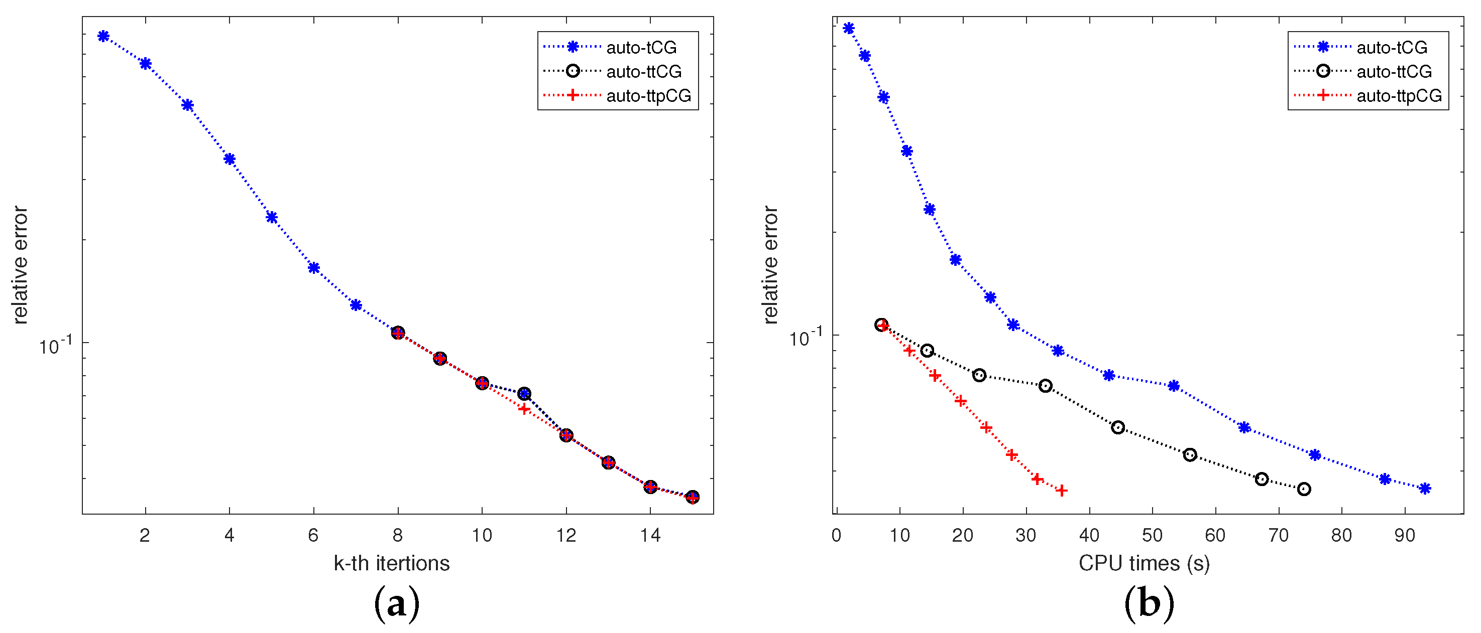
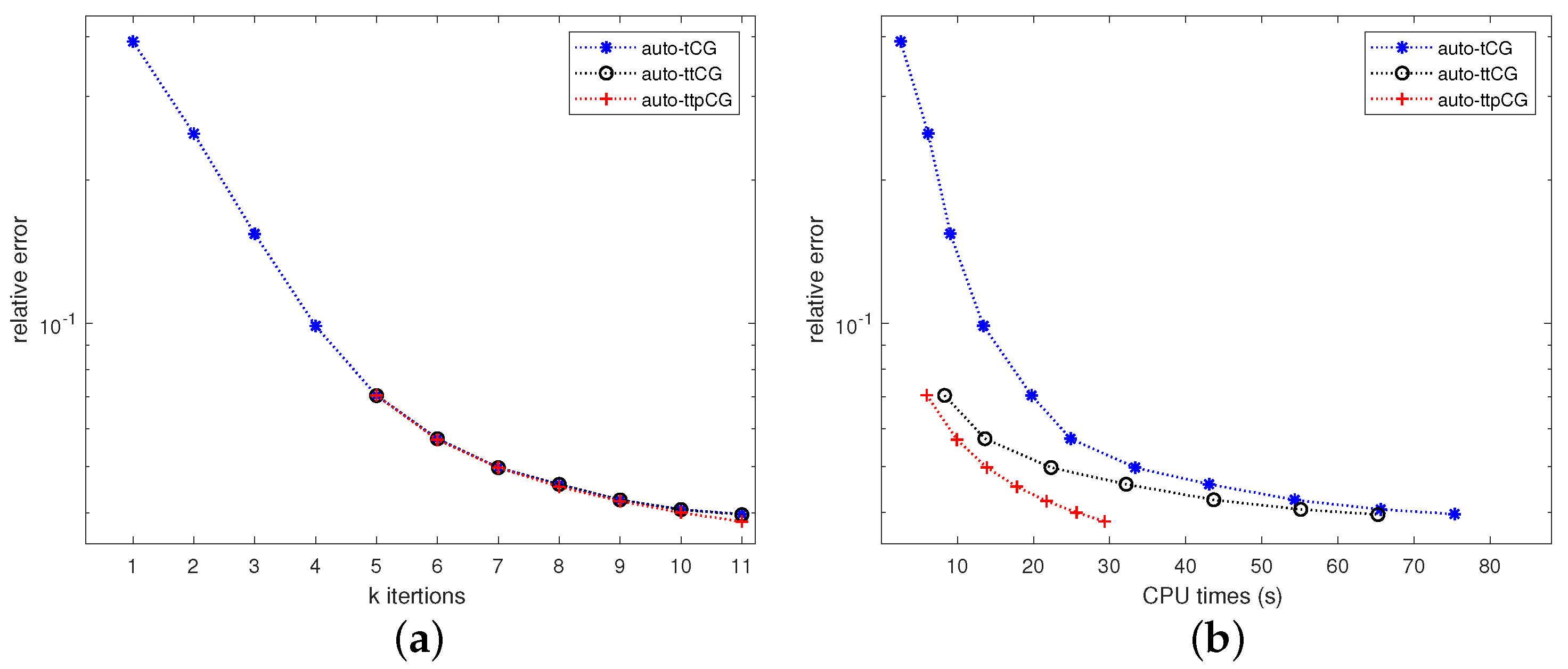
Figure 3 shows the convergence of relative errors verus (a) the iteration number k and (b) the CPU time for the tCG, auto-tCG, auto-ttCG and auto-ttpCG methods with the noise level $\nu ={10}^{-3}$ corresponding in

Table 2. Example 1: Comparison of relative error, SNR, and CPU time between the tCG with $\mu =1\times {10}^{-3}$, the A-tCG-FFT, A-CGLS-FFT, A-tpCG-FFT, auto-tCG, auto-ttCG and auto-ttpCG methods with different noise level $\nu ={10}^{-i},i=2,3$.

Noise Level	Method	k	${\mathit{\mu }}_{\mathit{k}}$	Relative Error	SNR	CPU (s)
${10}^{-3}$	tCG	-	1 $\times {10}^{-3}$	9.14 $\times {10}^{-2}$	12.21	9.87
	A-tCG-FFT	-	-	5.44 $\times {10}^{-2}$	18.63	88.02
	A-tCGLS-FFT	-	-	5.44 $\times {10}^{-2}$	18.63	82.23
	A-tPCG-FFT	-	-	5.42 $\times {10}^{-2}$	18.67	76.09
	auto-tCG	15	1.96 $\times {10}^{-5}$	3.54 $\times {10}^{-2}$	22.36	109.87
	auto-ttCG	15	1.96 $\times {10}^{-5}$	3.52 $\times {10}^{-2}$	22.41	80.93
	auto-ttpCG	15	1.96 $\times {10}^{-5}$	3.49 $\times {10}^{-2}$	22.48	33.98
${10}^{-2}$	tCG	-	1 $\times {10}^{-3}$	1.17 $\times {10}^{-1}$	11.97	9.64
	A-tCG-FFT	-	-	1.04 $\times {10}^{-2}$	12.75	79.33
	A-tCGLS-FFT	-	-	1.04 $\times {10}^{-2}$	12.75	72.29
	A-tPCG-FFT	-	-	9.81 $\times {10}^{-2}$	12.90	61.75
	auto-tCG	11	3.14 $\times {10}^{-4}$	8.74 $\times {10}^{-2}$	14.51	81.94
	auto-ttCG	11	3.14 $\times {10}^{-4}$	8.64 $\times {10}^{-2}$	14.61	26.42
	auto-ttpCG	11	3.14 $\times {10}^{-4}$	8.54 $\times {10}^{-2}$	14.72	18.50

. The iteration process is terminated when the discrepancy principle is satisfied. From Figure 3a, we can see that the auto-ttCG and auto-ttpCG methods do not need to solve the normal equation for all ${\mu }_k(k<8)$. This shows that the auto-ttCG and auto-ttpCG methods improve the auto-tCG method by Condition (24). Figure 3b shows that the auto-ttpCG method converges fastest among three methods.

Table 2 lists the regularization parameter, the iteration number, the relative error, SNR and the CPU time of the optimal solution obtained by using the tCG, A-tCG-FFT, A-CGLS-FFT, A-tpCG-FFT, auto-tCG, auto-ttCG and auto-ttpCG methods with different noise levels $\nu ={10}^{-i},i=2,3$. The determination of the regularization parameter for the tCG method involved conducting several experiments to obtain a more appropriate value. The CPU time represents only the usage in a single CG process.

The image restoration experiment of Example 1, the A-tCG-FFT, A-CGLS-FFT, and A-tpCG-FFT methods proposed by Song et al. [31] project the t-product into the Fourier domain and solve 256 ill-posed problems in matrix form, respectively. In Song et al.’s setting, when the frontal slice is small, the time required is very small. In the setting of our article, the number of frontal slices is related to the size of the image. As the number of frontal slices increases, the time cost increases. The calculation process of auto-tCG, auto-ttCG and auto-ttpCG methods always maintains the tensor t-product structure, resulting in higher quality image restoration in the end. The quality of the regularization solution obtained by the auto-tCG surpasses that of the solution obtained by the tCG method. It can be seen from Table 2 that the auto-ttpCG method has the lowest relative error, highest SNR and the least CPU time for different noise level.

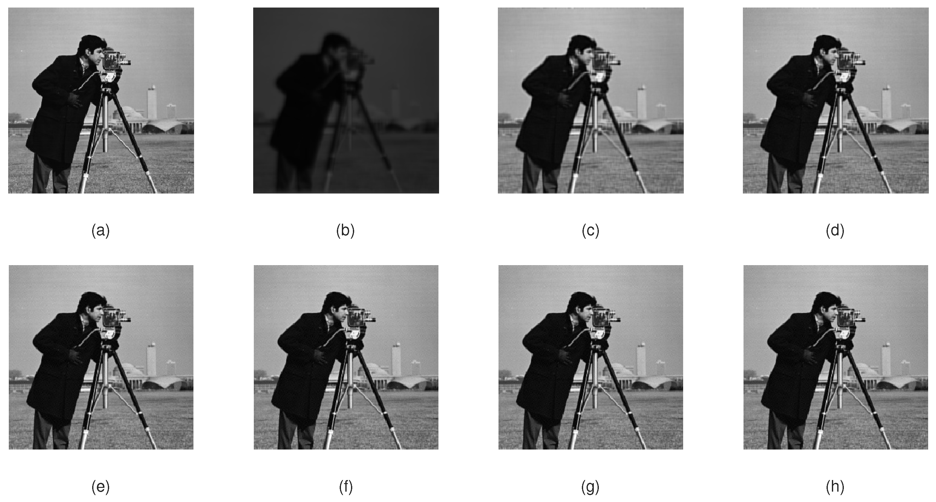
Figure 4 shows the reconstructed images obtained by using the tCG, A-tCG-FFT, A-CGLS-FFT, auto-tCG, auto-ttCG and auto-ttpCG methods on the blurred and noised image with the noise level $\nu ={10}^{-3}$ in Table 2. From Figure 4, we can see that the restored image by the auto-ttpCG method looks a bit better than others but with the least CPU time. The image restoration performance of the tCG method is inferior to three conjugate gradient methods with automatically determined parameters.

Example 2

(Color image). This example illustrates the restoration of a blurred $\mathbf{Lena}$ color image using Algorithms 3, 4 and 6. The original $\mathbf{Lena}$ image ${\mathcal{X}}_{ori}\in {\mathbb{R}}^{256\times 256\times 3}$ is stored as a tensor ${\mathcal{X}}_{true}\in {\mathbb{R}}^{256\times 3\times 256}$ through the MATLAB function ${\mathbf{multi}}_{-}\mathbf{twist}$. We set $N=256,\sigma =3$ and band = 12, and obtain $\mathcal{A}\in {\mathbb{R}}^{256\times 256\times 256}$ by

$$z=\left[exp(-\left(\left[0:band-1\right]{.}^2\right)/\left(2{\sigma }^2\right)),zeros(1,N-band)\right],$$

$$A=toeplitz\left(z\right),{\mathcal{A}}_{\left(:,:,i\right)}=\frac{1}{2\pi \sigma }A\left(i,1\right)A,i=1,\dots ,256.$$

Then, $cond\left({\mathcal{A}}_{(:,:,1)}\right)=\cdots =cond\left({\mathcal{A}}_{(:,:,12)}\right)=4.68e+07$, and the condition number of other tensor slices of $\mathcal{A}$ is infinite. The noise tensor $\mathcal{E}$ is defined by (36). The blurred and noised tensor is derived by $\mathcal{B}=\mathcal{A}\ast {\mathcal{X}}_{true}+\mathcal{E}$, which is shown in Figure 5b.

We set color image $\mathcal{B}$ to be divided into multiple lateral slices and independently process each slice through (1) by using the tCG, auto-tCG, auto-ttCG and auto-ttpCG methods. Figure 6 shows the convergence of relative errors verus (a) the iteration number k and (b) the CPU time for the auto-tCG, auto-ttCG and auto-ttpCG methods when dealing with the first tensor lateral slice ${\mathcal{B}}_{(:,1,:)}$ of $\mathcal{B}$ with $\nu ={10}^{-3}$. Similar results can be derived as that in Example 1 from Figure 6. We can see that the auto-ttCG and auto-ttpCG methods need less iterations than the auto-tCG method from Figure 6a and the auto-ttpCG method converges fastest among all methods from Figure 6b.

Table 3. Example 2: Comparison of relative error, SNR, and CPU time between the tCG ($\nu ={10}^{-2}$: $\mu =0.01$; $\nu ={10}^{-3}$: $\mu =0.005$), the A-tCG-FFT, A-CGLS-FFT and A-tpCG-FFT, auto-tCG, auto-ttCG and auto-ttpCG methods with different noise levels $\nu ={10}^{-i},i=2,3$.

Noise Level	Method	Relative Error	SNR	Time (s)
${10}^{-3}$	tCG	8.90 $\times {10}^{-2}$	11.15	34.73
	A-tCG-FFT	7.34 $\times {10}^{-2}$	13.39	6939.36
	A-tCGLS-FFT	7.34 $\times {10}^{-2}$	13.39	5634.69
	A-tPCG-FFT	7.34 $\times {10}^{-2}$	13.39	1638.91
	auto-tCG	5.90 $\times {10}^{-2}$	14.62	314.73
	auto-ttCG	5.90 $\times {10}^{-2}$	14.62	262.81
	auto-ttpCG	5.43 $\times {10}^{-2}$	15.37	103.41
${10}^{-2}$	tCG	9.64 $\times {10}^{-2}$	10.23	31.63
	A-tCG-FFT	8.98 $\times {10}^{-2}$	11.01	5236.55
	A-tCGLS-FFT	8.98 $\times {10}^{-2}$	11.01	4895.52
	A-tPCG-FFT	8.98 $\times {10}^{-2}$	11.01	1236.21
	auto-tCG	7.64 $\times {10}^{-2}$	12.37	117.48
	auto-ttCG	7.48 $\times {10}^{-2}$	12.55	62.01
	auto-ttpCG	7.01 $\times {10}^{-2}$	13.13	54.85

lists the relative error, SNR and the CPU time of the optimal solution obtained by using the tCG, A-tCG-FFT, A-CGLS-FFT, A-tpCG-FFT, auto-tCG, auto-ttCG and auto-ttpCG methods with different noise levels $\nu ={10}^{-i},i=2,3$. The results are very similar to that in Table 2 for different noise levels. In the application of the tCG method, we define distinct regularization parameters, specifically setting $\mu =0.01$ when $\nu ={10}^{-2}$, and $\mu =0.005$ when $\nu ={10}^{-3}$. The regularization parameter set for the tCG method has been determined through multiple iterations, yielding a reasonably suitable value. However, when applying tCG to solve Problem (9) corresponding to other regularization parameters attempted during this process, divergence or excessively large relative errors are commonly observed. When the condition number for frontal slicing is larger, the condition number for the matrix projected into the Fourier domain also increases, which leads to increased ill-posedness and results in more CPU time for the A-tCG-FFT, A-CGLS-FFT and A-tpCG-FFT methods to obtain regularization parameters. The quality of the solutions obtained by the tCG method is inferior to that of the other three versions with automatic parameter tuning. However, the CPU time used by the tCG method is shorter than the other three methods. This is because it only represents the time spent solving a regularized equation, whereas the process of manually selecting regularization parameters would consume more time. Table 3 also reflects the advantages of both truncation parameters and preprocessing operations.

Figure 5 shows the recovered images by the tCG, A-tCG-FFT, A-CGLS-FFT, auto-tCG, auto-ttCG and auto-ttpCG methods corresponding to the results with noise level $\nu ={10}^{-3}$. The results are very similar to that in Figure 5.

Example 3

(Video). In this example, we employ three distinct reconstruction methods on MATLAB to recover the initial 10 consecutive frames of the blurred and noisy $\mathbf{Rhinos}$ video, with each frame containing $240\times 240$ pixels. We store ten frames devoid of pollution and noise from the original video in the tensor ${\mathcal{X}}_{true}\in {\mathbb{R}}^{240\times 10\times 240}$. We let z be defined by (37) with $N=240$, $\sigma =2$ and $band=12$. The coefficient tensor $\mathcal{A}$ is defined as follows:

$$A=\frac{1}{\sqrt{2\pi \sigma }}toeplitz\left(z\right),{\mathcal{A}}_{\left(:,:,i\right)}=A\left(i,1\right)A,i=1,\dots ,240.$$

The condition number of the frontal slices of $\mathcal{A}$ is $cond\left({\mathcal{A}}_{(:,:,i)}\right)=7.4484e+09(i\le 12)$, and the condition number of the remaining frontal sections of $\mathcal{A}$ is infinite. The suitable regularization parameter is determined by using the discrepancy principle with $\eta =1.1$. The blurred and noised tensor $\mathcal{B}$ is generated by $\mathcal{B}=\mathcal{A}\ast {\mathcal{X}}_{true}+\mathcal{E}$ with $\mathcal{E}\in {\mathbb{R}}^{120\times 30\times 120}$ being defined by (36).

Figure 7 shows the convergence of relative errors verus the iteration number k and relative errors verus the CPU time for the auto-tCG, auto-ttCG and auto-ttpCG methods when the second frame of the video with $\nu ={10}^{-3}$ is restored. Very similar results can be derived from Figure 7 to that in Example 1.

Table 4. Example 3: Comparison of relative error, SNR, and CPU time between the tCG ($\nu ={10}^{-2}$: $\mu =0.05$; $\nu ={10}^{-3}$: $\mu =0.001$), the A-tCG-FFT, A-CGLS-FFT, A-tpCG-FFT, auto-tCG, auto-ttCG and auto-ttpCG methods with different noise level $\nu ={10}^{-i},i=2,3$.

Noise Level	Method	Relative Error	SNR	Time (s)
${10}^{-3}$	tCG	3.94 $\times {10}^{-2}$	21.43	96.33
	A-tCG-FFT	3.67 $\times {10}^{-2}$	21.95	9396.36
	A-tCGLS-FFT	3.67 $\times {10}^{-2}$	21.95	7423.69
	A-tPCG-FFT	3.67 $\times {10}^{-2}$	21.95	3798.81
	auto-tCG	2.94 $\times {10}^{-2}$	23.17	697.78
	auto-ttCG	2.92 $\times {10}^{-2}$	23.23	487.35
	auto-ttpCG	2.66 $\times {10}^{-2}$	24.05	214.16
${10}^{-2}$	tCG	8.31 $\times {10}^{-2}$	14.14	80.61
	A-tCG-FFT	7.89 $\times {10}^{-2}$	14.89	8972.69
	A-tCGLS-FFT	7.89 $\times {10}^{-2}$	14.89	7263.02
	A-tPCG-FFT	7.89 $\times {10}^{-2}$	14.89	3269.36
	auto-tCG	5.24 $\times {10}^{-2}$	18.15	480.75
	auto-ttCG	5.10 $\times {10}^{-2}$	18.38	281.54
	auto-ttpCG	4.74 $\times {10}^{-2}$	19.02	156.44

displays the relative error, SNR and the CPU time of the optimal solution obtained by using the tCG, the A-tCG-FFT, A-CGLS-FFT, A-tpCG-FFT, auto-tCG, auto-ttCG and auto-ttpCG methods for the second frame with different noise levels $\nu ={10}^{-i}$, $i=2,3$. In video restoration experiments with continuous frames, using the A-tCG-FFT, A-CGLS-FFT, A-tpCG-FFT methods to perform matrix calculations in the Fourier domain may cause a certain degree of damage to the spatial structure that may exist between consecutive frames, resulting in a decrease in restoration quality. When employing the tCG method, we configured distinct regularization parameters, specifically, when $\nu ={10}^{-2}$, $\mu =0.05$; and when $\nu ={10}^{-3}$, $\mu =0.001$. With the increase in data volume, the auto-tCG method demonstrates better solution quality compared to the tCG method. Additionally, the truncation parameter operation and preprocessing strategy exhibit superior solution quality and time advantages over auto-tCG. We can see that the auto-ttpCG method has the largest SNR and the lowest CPU time for different noise level $\nu ={10}^{-i},i=2,3$.

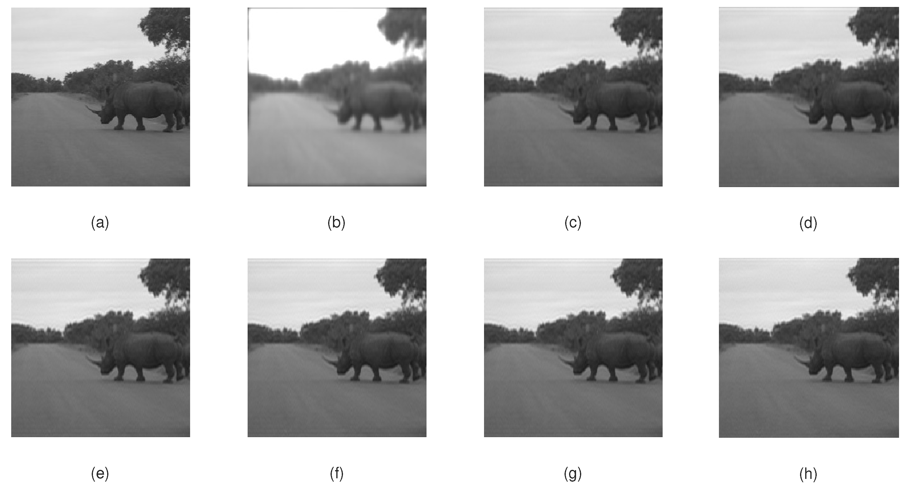
Figure 8 shows the original video, blurred and noised video, and the recovered video of the second frame of the video for the tCG, A-tCG-FFT, A-CGLS-FFT, A-tCG-FFT, A-CGLS-FFT, auto-tCG, auto-ttCG and the auto-ttpCG methods with noise level $\nu ={10}^{-3}$ corresponding to the results in Table 4. The recovered frame by the auto-ttpCG method looks best among all recovered frames.

5. Conclusions

This paper introduces three tensor Conjugate Gradient methods designed for the resolution of large-scale linear discrete ill-posed problems formulated in tensor representation. Initially, we introduce an automated strategy for determining an appropriate regularization parameter for the tensor Conjugate Gradient (tCG) method. Furthermore, we develop a truncated version and a preprocessed version of the tCG method. The introduced methodologies are employed in diverse instances of image and video restoration. The efficacy of the proposed methodologies in image and video restoration applications is demonstrated through illustrative examples. These approaches circumvent the need for problem matrixization or vectorization. Notably, these methods exhibit significant potential in terms of both speed and quality of computed restoration, as assessed by relative errors and SNR values, providing a comprehensive evaluation of algorithmic performance in image restoration.

References

1. Reichel, L.; Ugwu, U.O. The tensor Golub–Kahan–Tikhonov method applied to the solution of ill-posed problems with at-product structure. Numer. Linear Algebr. Appl. 2022, 29, e2412. [Google Scholar] [CrossRef]
2. Ugwu, U.O.; Reichel, L. Tensor Arnoldi–Tikhonov and GMRES-Type Methods for Ill-Posed Problems with a t-Product Structure. J. Sci. Comput. 2022, 90, 1–39. [Google Scholar]
3. Cichocki, A.; Mandic, D.; De Lathauwer, L.; Zhou, G.; Zhao, Q.; Caiafa, C.; Phan, H.A. Tensor decompositions for signal processing applications: From two-way to multiway component analysis. IEEE Signal Process. Mag. 2015, 32, 145–163. [Google Scholar] [CrossRef]
4. Signoretto, M.; Tran Dinh, Q.; De Lathauwer, L.; Suykens, J.A. Learning with tensors: A framework based on convex optimization and spectral regularization. Mach. Learn. 2014, 94, 303–351. [Google Scholar] [CrossRef]
5. Kilmer, M.E.; Horesh, L.; Avron, H.; Newman, E. Tensor-tensor algebra for optimal representation and compression of multiway data. Proc. Natl. Acad. Sci. USA 2021, 118, e2015851118. [Google Scholar] [CrossRef] [PubMed]
6. Beik, F.P.A.; Najafi–Kalyani, M.; Reichel, L. Iterative Tikhonov regularization of tensor equations based on the Arnoldi process and some of its generalizations. Appl. Numer. Math. 2020, 151, 425–447. [Google Scholar] [CrossRef]
7. Bentbib, A.H.; Khouia, A.; Sadok, H. The LSQR method for solving tensor least-squares problems. Electron. Trans. Numer. Anal. 2022, 55, 92–111. [Google Scholar] [CrossRef]
8. Zheng, M.M.; Ni, G. Approximation strategy based on the T-product for third-order quaternion tensors with application to color video compression. Appl. Math. Lett. 2023, 140, 108587. [Google Scholar] [CrossRef]
9. Kilmer, M.E.; Martin, C.D. Factorization strategies for third order tensors. Linear Alg. Appl. 2011, 435, 641–658. [Google Scholar] [CrossRef]
10. Hao, N.; Kilmer, M.E.; Braman, K.; Hoover, R.C. Facial recognition using tensor-tensor decompositions. SIAM J. Imaging Sci. 2013, 6, 437–463. [Google Scholar] [CrossRef]
11. Kilmer, M.E.; Braman, K.; Hao, N.; Hoover, R.C. Third-order tensors as operators on matrices: A theoretical and computational framework with applications in imaging. SIAM J. Matrix Anal. Appl. 2013, 34, 148–172. [Google Scholar] [CrossRef]
12. Bentbib, A.H.; El Hachimi, A.; Jbilou, K.; Ratnani, A. Fast multidimensional completion and principal component analysis methods via the cosine product. Calcolo 2022, 59, 26. [Google Scholar] [CrossRef]
13. Khaleel, H.S.; Sagheer, S.V.M.; Baburaj, M.; George, S.N. Denoising of Rician corrupted 3D magnetic resonance images using tensor-SVD. Biomed. Signal Process. Control 2018, 44, 82–95. [Google Scholar] [CrossRef]
14. Zeng, C.; Ng, M.K. Decompositions of third-order tensors: HOSVD, T-SVD, and Beyond. Numer. Linear Algebr. Appl. 2020, 27, e2290. [Google Scholar] [CrossRef]
15. El Hachimi, A.; Jbilou, K.; Ratnani, A.; Reichel, L. Spectral computation with third-order tensors using the t-product. Appl. Numer. Math. 2023, 193, 1–21. [Google Scholar] [CrossRef]
16. Yu, Q.; Zhang, X. T-product factorization based method for matrix and tensor completion problems. Comput. Optim. Appl. 2023, 84, 761–788. [Google Scholar] [CrossRef]
17. Tikhonov, A.N.; Arsenin, V.Y. Solutions of Ill-Posed Problems; Transl. from Russian; V.H. Winston & Sons: Washington, DC, USA, 1977. [Google Scholar]
18. Fenu, C.; Reichel, L.; Rodriguez, G. GCV for tikhonov regularization via global Golub–Kahan decomposition. Numer. Linear Algebr. Appl. 2016, 25, 467–484. [Google Scholar] [CrossRef]
19. Hansen, P.C. Rank-deficient and Discrete Ill-posed Problems: Numerical Aspects of Linear Inversion. SIAM J. Sci. Comput. 1998, 20, 684–696. [Google Scholar]
20. Kindermann, S. Convergence analysis of minimization-based noise level-free parameter choice rules for linear ill-posed problems. Electron. Trans. Numer. Anal. 2011, 38, 233–257. [Google Scholar]
21. Kindermann, S.; Raik, K. A simplified L-curve method as error estimator. Electron. Trans. Numer. Anal. 2020, 53, 217–238. [Google Scholar] [CrossRef]
22. Reichel, L.; Rodriguez, G. Old and new parameter choice rules for discrete ill-posed problems. Numer. Algorithms 2013, 63, 65–87. [Google Scholar] [CrossRef]
23. Engl, H.W.; Hanke, M.; Neubauer, A. Neubauer. In Regularization of Inverse Problems; Kluwer: Dordrecht, The Netherlands, 1996. [Google Scholar]
24. Zhang, J.; Saibaba, A.K.; Kilmer, M.E.; Aeron, S. A randomized tensor singular value decomposition based on the t-product. Numer. Linear Algebr. Appl. 2018, 25, e2179. [Google Scholar] [CrossRef]
25. Ugwu, U.O.; Reichel, L. Tensor regularization by truncated iteration: A comparison of some solution methods for large-scale linear discrete ill-posed problem with a t-product. arXiv 2021, arXiv:2110.02485. [Google Scholar]
26. Hestenes, M.R.; Stiefel, E. Methods of conjugate gradients for solving linear systems. J. Res. Natl. Bur. Stand. 1952, 49, 409–436. [Google Scholar] [CrossRef]
27. Polyak, B.T. The conjugate gradient method in extremal problems. U.S.S.R. Comput. Math. Math. Phys. 1969, 9, 94–112. [Google Scholar] [CrossRef]
28. Gilbert, J.C.; Nocedal, J. Global convergence properties of conjugate gradient methods for optimization. SIAM J. Optim. 1992, 2, 21–42. [Google Scholar] [CrossRef]
29. Nocedal, J.; Wright, S.J. Numerical Optimization; Springer: New York, NY, USA, 1999. [Google Scholar]
30. Saad, Y. Iterative Methods for Sparse Linear Systems; SIAM: Philadelphia, PA, USA, 2003. [Google Scholar]
31. Song, H.M.; Wang, S.W.; Huang, G.X. Tensor Conjugate-Gradient methods for tensor linear discrete ill-posed problems. AIMS Math. 2023, 8, 26782–26800. [Google Scholar] [CrossRef]
32. Lund, K. The tensor t-function: A definition for functions of third-order tensors. Numer. Linear Algebr. Appl. 2020, 27, e2288. [Google Scholar] [CrossRef]
33. Frommer, A.; Maass, P. Fast CG-based methods for Tikhonov–Phillips regularization. SIAM J. Sci. Comput. 1999, 20, 1831–1850. [Google Scholar] [CrossRef]
Figure 1. (a) Frontal slices A ( : , : , k ) , (b) lateral slices A ( : , j , : ) and (c) tube fibers A ( i , j , : ) .
Mathematics 12 00159 g001
Figure 2. Twist squeeze.
Mathematics 12 00159 g002
Figure 3. Example 1: Comparison of convergence between (a) relative errors verus the iteration number k and (b) relative errors verus the CPU time for the auto-tCG, auto-ttCG and auto-ttpCG methods with the noise level ν = 10 3 .
Mathematics 12 00159 g003
Figure 4. Example 1: (a) The original image and (b) the blurred and noised image, reconstructed images by (c) the tCG method (SNR = 12.21, CPU = 9.87), (d) the A-tCG-FFT method (SNR = 18.63, CPU = 88.02), (e) the A-CGLS-FFT method (SNR = 18.63, CPU = 82.23), (f) the auto-tCG method (SNR = 22.36, CPU = 109.87), (g) the auto-ttCG method (SNR = 22.41, CPU = 80.93) and (h) the auto-ttpCG method (SNR = 22.48, CPU = 33.98) according to the noise level ν = 10 3 in Table 2.
Mathematics 12 00159 g004
Figure 5. Example 2: (a) The original image Lena, (b) the blurred and noised image and reconstructed images by (c) the tCG method, (d) the A-tCG-FFT method, (e) the A-CGLS-FFT method, (f) the auto-tCG method, (g) the auto-ttCG and (h) the auto-ttpCG method according to the noise level ν = 10 3 in Table 3.
Mathematics 12 00159 g005
Figure 6. Example 2: Comparison of convergence between (a) relative errors verus the iteration number k and (b) relative errors verus the CPU time for the auto-tCG, auto-ttCG and auto-ttpCG methods with the noise level ν = 10 3 .
Mathematics 12 00159 g006
Figure 7. Example 3: Comparison of convergence between (a) relative errors verus the iteration number k and (b) relative errors verus the CPU time for the auto-tCG, auto-ttCG and auto-ttpCG methods with the noise level ν = 10 3 .
Mathematics 12 00159 g007
Figure 8. Example 3: (a) The second frame image of the original video, (b) the blurred and noisy image and recovered images by (c) the tCG method, (d) the A-tCG-FFT method, (e) the A-CGLS-FFT method, (f) the auto-tCG method, (g) the auto-ttCG and (h) the auto-ttpCG method according to the noise level ν = 10 3 in Table 4.
Mathematics 12 00159 g008