Instance Segmentation Frustum–PointPillars: A Lightweight Fusion Algorithm for Camera–LiDAR Perception in Autonomous Driving

Abstract

The fusion of camera and LiDAR perception has become a research focal point in the autonomous driving field. Existing image–point cloud fusion algorithms are overly complex, and processing large amounts of 3D LiDAR point cloud data requires high computational power, which poses challenges for practical applications. To overcome the above problems, herein, we propose an Instance Segmentation Frustum (ISF)–PointPillars method. Within the framework of our method, input data are derived from both a camera and LiDAR. RGB images are processed using an enhanced 2D object detection network based on YOLOv8, thereby yielding rectangular bounding boxes and edge contours of the objects present within the scenes. Subsequently, the rectangular boxes are extended into 3D space as frustums, and the 3D points located outside them are removed. Afterward, the 2D edge contours are also extended to frustums to filter the remaining points from the preceding stage. Finally, the retained points are sent to our improved 3D object detection network based on PointPillars, and this network infers crucial information, such as object category, scale, and spatial position. In pursuit of a lightweight model, we incorporate attention modules into the 2D detector, thereby refining the focus on essential features, minimizing redundant computations, and enhancing model accuracy and efficiency. Moreover, the point filtering algorithm substantially diminishes the volume of point cloud data while concurrently reducing their dimensionality, thereby ultimately achieving lightweight 3D data. Through comparative experiments on the KITTI dataset, our method outperforms traditional approaches, achieving an average precision (AP) of 88.94% and bird’s-eye view (BEV) accuracy of 90.89% in car detection.

1. Introduction

1.1. Motivation

Accurately and efficiently detecting obstacles is an essential requirement for autonomous vehicles. Mainstream sensors in the perception system include RGB cameras and LiDAR [1]. Cameras in autonomous driving present advantages such as cost-effectiveness, well-established technology, and the capability to capture detailed environmental information. However, cameras are susceptible to illumination and have limited accuracy. LiDAR offers high-ranging accuracy and strong directionality. However, it is associated with high hardware costs, a limited detection range, and challenges in extracting the obstacle category and texture feature information from point clouds. The fusion of camera and LiDAR data can achieve complementary advantages. Cameras provide high-resolution RGB images, thereby enabling precise obstacle classification, while distance detection with LiDAR offers accurate obstacle localization. However, the fusion of LiDAR and camera data introduces its own set of challenges [2]. The combined data from both sensors are substantial, particularly the real-time point cloud stream from LiDAR, which consumes significant CPU and storage resources. Moreover, fusion algorithms may encounter situations where the results from the two sensors do not align, thus leading to challenges in determining the reliability of each sensor’s output. To overcome the above shortcomings, we propose the ISF–PointPillars algorithm, which can significantly reduce the amount of LiDAR point cloud information, thus accounting for the central part of the data stream while ensuring the accuracy and reliability of the perception results, as well as preventing noise interference caused by multisensor fusion.

1.2. Related Work

1.2.1. Two-Dimensional Instance Segmentation

In 2D instance segmentation, a computer vision (CV) task, the aim is to identify and segment individual objects in an image [3]. This task involves detecting the boundaries of each object and assigning a unique label to them. It requires simultaneously handling both object detection and segmentation while dealing with objects of different classes, scales, poses, and levels of occlusion. Fully supervised instance segmentation based on deep learning can be divided into single-stage and two-stage methods [4].

Mask R-CNN [5] is a prominent two-stage instance segmentation method. In the initial stage, it generates candidate regions of interest (ROI), followed by the classification and segmentation of these ROIs in the subsequent stage. However, this approach exhibits drawbacks in terms of computational efficiency, thereby leading to prolonged training times for the model.

On the contrary, single-stage instance segmentation methods perform segmentation and detection simultaneously, which can significantly reduce inference time. Typical single-stage methods include YOLACT [6], SOLO [7], and PolarMask [8]. The core idea of YOLACT is to predict the prototype mask of the current picture and the mask coefficients of each bounding box (bbox) instance in parallel and then generate instance masks by linearly combining the prototype and the mask coefficients. This parallel prediction method can maintain high output resolution. This results in a relatively high segmentation accuracy.

The YOLOv8-Seg [9] model is a combination of YOLACT and the existing YOLOv8 detection updates, and it ranks high on the leaderboard of instance segmentation tasks. However, single-stage instance segmentation based on convolutional neural networks (CNNs) may not be able to generate fine masks when dealing with large objects featuring complex shapes, and its accuracy is low because all calculations must be completed using limited computing resources. In addition, although YOLOv8 has improved in many aspects when compared with the previous generations of the YOLO series, there are still some potential areas for improvement in image instance segmentation tasks. The first is computational complexity. The corresponding number of parameters and floating-point operations per second (FLOPS) of YOLOv8’s tiny, small, and large (N/S/M)-scale models has increased significantly compared to the previous generation. This means that YOLOv8 requires more computing resources and longer training and inference times, which may pose challenges in resource-limited environments. Secondly, in terms of inference speed, the inference speed of most YOLOv8 models has dropped compared to models of previous generations, which is highly detrimental to applications that require real-time processing, such as autonomous driving and video surveillance. In addition, regarding generalization capabilities, various YOLO series-improved algorithms now have significant performance improvements on the COCO dataset [10], but generalization on custom datasets has yet to be widely verified. This means that YOLOv8 may not achieve the expected performance on a specific task or dataset.

1.2.2. Attention Mechanism

The application of attention mechanisms in CV has made significant progress in recent years [11]. After introducing the attention mechanism, visual neural networks become more targeted when processing images. They assign different weights to each part of the feature map to extract more critical information, thereby improving the accuracy of the results.

The transformer-based CV target detection method is a current research focal point [12]; however, the CNN-based method cannot yet be entirely replaced. One of the essential reasons is computational efficiency. Most transformer-based methods directly apply the transformer structure in natural language processing (NLP) and rarely make specific designs for CV data. However, we know images and videos contain far more information than text, thus exerting enormous computational pressure when applying self-attention networks to process them. Autonomous driving systems have significant real-time requirements and limited onboard computing resources; thus, these kinds of algorithms are difficult to widely popularize.Moreover, transformer-based target detection networks can achieve superior performance over CNN-based methods only when relying on extremely large-scale datasets. In the case of medium-sized datasets, such as KITTI [13], the transformer model fails to demonstrate its advantages.

Unlike the transformer, which focuses on processing sequence data, a spatial attention mechanism is mainly combined with CNN. Representative methods of this type include EMA [14], NAM [15], SA [16], ECA [17], CA [18], etc., which mainly focus on local dependencies in the feature map. The EMA module outperforms other attention methods with fewer parameters. It reshapes the channel dimensions and groups them into multiple subfeatures to distribute spatial semantic features. Moreover, the EMA module uses multiscale parallel subnetworks to establish short and long dependencies. It fuses the output feature maps of the two parallel subnetworks through a cross-space learning method. Additionally, this module reshapes part of the channel into batch dimensions to avoid some form of dimensionality reduction via universal convolution. The combined effect of the above characteristics helps improve the model’s performance, thereby enhancing its ability to capture image details, process complex structures, and infer target boundaries. To conclude, EMA achieves better results and is more efficient in terms of the required parameters. As an illustration, EMA has been shown to improve the baseline performance of target detection when the YOLOv5x model [19] was used as the backbone for target detection on the VisDrone dataset [20].

1.2.3. Three-Dimensional Detection

Unlike 2D object detection, which concentrates on object identification in images, the essence of 3D object detection lies in its endeavor to precisely ascertain real-world objects’ 3D placements, extents, and alignments [21]. Currently, the mainstream 3D detection algorithm in autonomous driving is based on the LiDAR point cloud.

Point-based 3D target detection algorithms retain the unstructured form of the point cloud, preserve the information of the original point cloud to the greatest extent, and adapt the sampling strategy as needed [22]. However, this method is computationally expensive and may introduce random sampling bias.

The voxel-based 3D detection method assigns points to voxels, thereby dividing the LiDAR point cloud with fixed-sized voxels in 3D spaces [23]. This method reduces computational complexity, but improper selection of the voxel size may cause information loss.

The method based on pillars is to divide the grid along the x and y axes of the 3D space and then stretch each grid on the z axis to cover the entire space. Then, each point is divided into a particular pillar, and an encoder converts the pillars into a 2D pseudoimage, which can be further processed via the 2D CNN. PointPillars [24] is a widely favored 3D target detection solution for autonomous driving. It achieves a commendable trade-off between speed and precision, thus earning recognition for its swift execution, high accuracy, and ease of deployment. However, the generalization of PointPillars needs to be improved, since focal loss [25] is used as the classification loss function. In addition, the data for each point include four dimensions: x, y, z, and reflectivity. An increase in the number of information dimensions results in a higher computational load for the neural network.

1.2.4. Multiple Sensor Fusion

Methods for fusing camera and LiDAR perception for obstacle detection in autonomous driving include early fusion, late fusion, and multistage fusion methods.

The early fusion approach utilizes a single neural network to process information from multiple sensors. Examples of this approach include PointPainting [26] and LIF-Seg [27]. While the early fusion method ensures detection accuracy, a failure in a single sensor can impact the entire system.

As for the late fusion method, which is also called separated fusion, each sensor has its dedicated network for processing, and the results are subsequently fused. Examples of this approach are CLOCs [28] and DeepFusion [29]. However, this approach requires more computational resources, thereby leading to increased latency, which is detrimental to real-time performance.

The multistage method involves stacking different modality neural networks together, with the output from the front network serving as input to the subsequent network. Examples include F-PointNet [30], F-ConvNet [31], and F-PointPillars [32]. This method combines multiple complementary tasks, such as object detection, instance segmentation, and depth completion [33], to achieve superior overall performance while reducing computational costs. Nonetheless, the multistage method also has areas worthy of improvement. F-PointPillars uses a 2D detection network to obtain a rectangular bbox of each obstacle, generates elliptical Gaussian masks within each bbox, and only retains the corresponding 3D space point cloud within the Gaussian mask to reduce background points. This improves computational efficiency; however, Gaussian masks cannot reflect the actual shape of obstacles. The rough point filtering method will inevitably discard points belonging to obstacles, and completely removing the background points is impossible, thus negatively affecting the target detection results. In recent times, 2D image instance segmentation algorithms have developed rapidly, and the inference speed and accuracy have been continuously enhanced. Refined instance segmentation frames can be extrapolated into 3D space to generate frustums and filter points. This process enables the retention of points exclusively associated with obstacles while systematically eliminating background point clouds to a maximal extent. Consequently, this enhancement significantly contributes to the precision of the 3D target detection network. Accordingly, our study has been conducted under the premise of this critical assumption.

1.3. Contributions

In summary, the contributions of ISF–PointPillars are as follows:

(1)

We leveraged 2D instance segmentation masks to create frustums to eliminate 3D background point clouds.

Compared to methods using rectangular boxes and Gaussian masks, our method achieved greater accuracy, effectively retained obstacle point clouds, maximally removed background points, and improved the performance of 3D detectors.

(2)

After comparative experiments, we selected the YOLOv8 framework as the basis of the 2D target detection network. We incorporated EMA into the YOLOv8 network, enhanced its backbone using C2F-FE, and employed a slim-neck structure to optimize the detection head. These modifications significantly improved the detection performance, particularly in autonomous driving scenarios.

(3)

We chose PointPillars as the 3D LiDAR object detection method through comparative analysis. Subsequently, we enhanced its network architecture to accommodate fusion algorithms and fine-tuned the model to adapt to the KITTI dataset.

2. Method

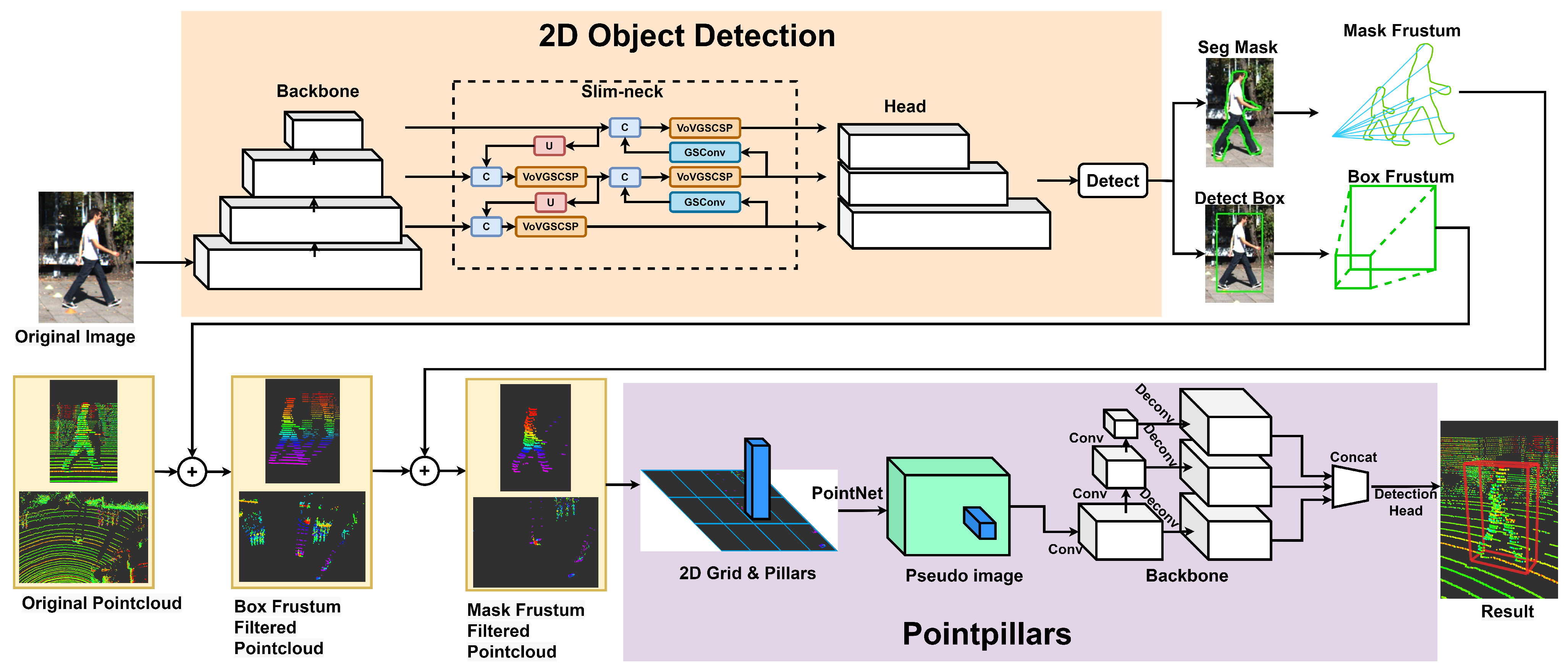
In this section, we present the ISF–PointPillars method, as depicted in Figure 1. The RGB image is initially fed into the 2D target detection network, thus generating multiple-scale feature maps via the backbone. Subsequently, multilevel features are fused through the slim-neck structure. The outputs, including the bounding box and instance segmentation mask, are then generated via the target detection head and instance segmentation head, respectively. The bounding box is extended to 3D space to generate a frustum, and the point data are roughly filtered. Then, the instance mask is extended to 3D space to generate an instance contour frustum, and the point cloud is finely filtered again. After undergoing two filtering processes, the remaining point count is significantly reduced. Finally, the remaining point cloud is fed into the enhanced PointPillars network for inference, thereby yielding information about the object’s category, scale, position, and orientation.

The algorithm proposed in this study is validated for 2D and 3D detection performance on the KITTI dataset. Qualitative and ablation experiments are conducted to verify the effectiveness of each step in the proposed workflow. The experimental results demonstrate that the innovative contributions introduced in this study effectively enhanced detection accuracy.

2.1. Instance Frustum Filter

This section introduces an effective method to significantly reduce the quantity of 3D spatial point cloud data while maximally preserving the points belonging to target objects. In the 3D LiDAR point cloud, the points belonging to the objects of interest, such as cars, cyclists, and pedestrians, are referred to as “foreground points”, while the points belonging to areas of disinterest such as roads, buildings, and green spaces are termed “background points”.

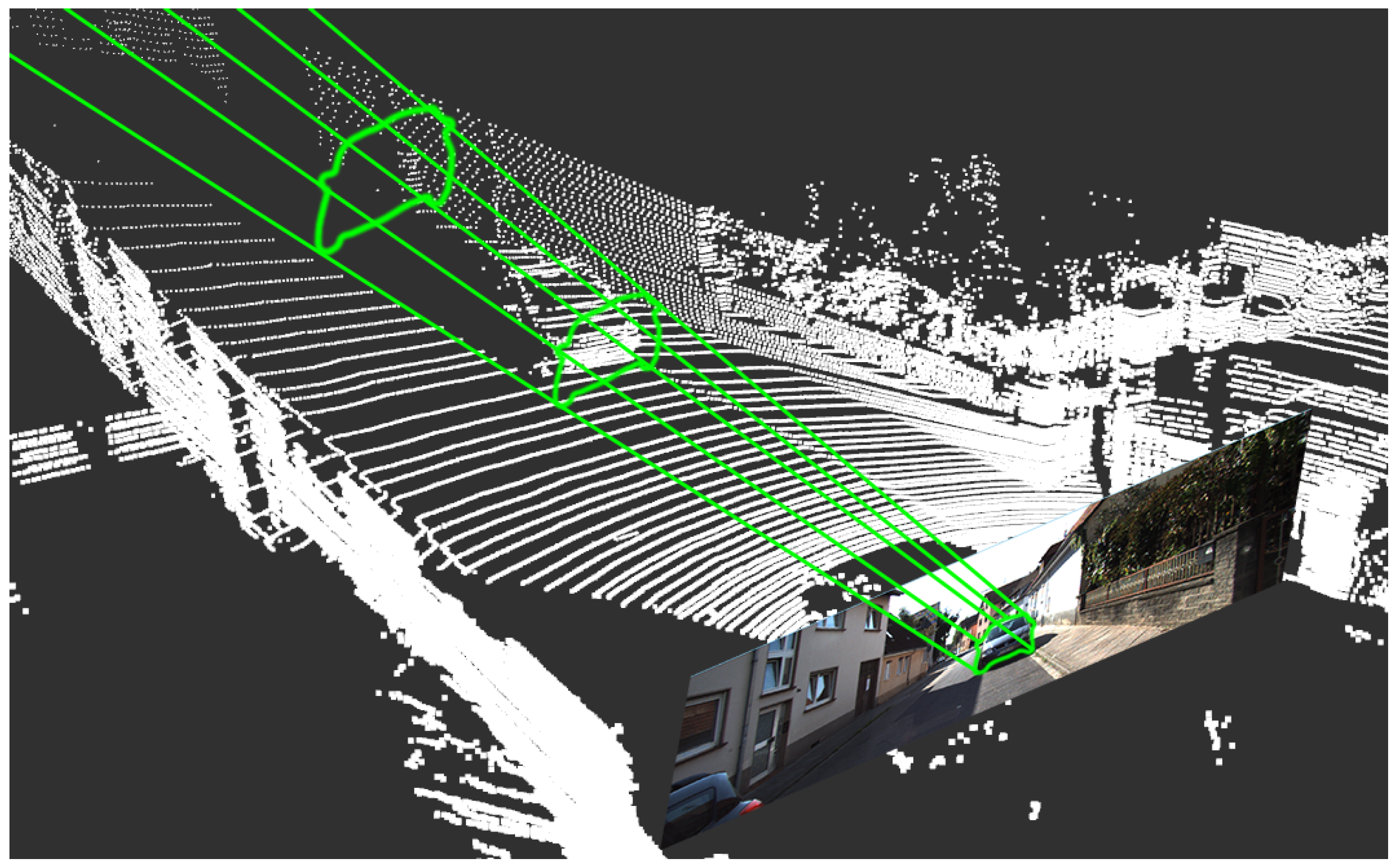
We drew inspiration from the method of generating frustums using rectangular bounding boxes [32] and introduced innovative modifications to it. By extending the boundaries of 2D image instance segmentation into 3D frustums, as illustrated in Figure 2, and employing the ray casting algorithm [34], we could effectively filter out nearly all background points located outside these frustums. This results in a reduced data volume sent into the 3D network and improved object detection accuracy.

It is worth noting that our point cloud segmentation algorithm has apparent advantages over traditional ones. First, our method can accurately identify and remove background points, thereby retaining more useful information. In contrast, voxel downsampling and random downsampling may lose some important point cloud details. Moreover, our method eliminates the need for additional parameter settings. In contrast, techniques such as voxel downsampling and random downsampling may necessitate adjustments to parameters, such as the voxel size or sampling ratio. Additionally, ground segmentation algorithms may require tuning multiple parameters based on specific environments, which is a time-consuming and labor-intensive process. Furthermore, our method does not depend on the structure and density of the point cloud, thus making it applicable to a wider range of scenarios.

The specific implementation process of the algorithm is as follows:

First, we establish the corresponding relationship between 3D LiDAR points and 2D RGB images. Mapping any point $\mathrm{x}={(x,y,z,1)}^T$ in 3D LiDAR point cloud space to its corresponding point $\mathrm{y}={(u,v,1)}^T$ on the camera image can be achieved using the following equation:

$$\mathrm{y}={\mathrm{P}}_{rect}^{\left(i\right)}{\mathrm{R}}_{rect}^{\left(0\right)}{\mathrm{T}}_{velo}^{cam}\mathrm{x}$$

(1)

where ${\mathrm{P}}_{rect}^{\left(i\right)}\in {\mathbb{R}}^{3\times 4}$ is the rectified projection matrix of the ith camera, and ${\mathrm{R}}_{rect}^{\left(i\right)}\in {\mathbb{R}}^{3\times 3}$ is the rectified rotation matrix. Here, ${\mathrm{R}}_{rect}^{\left(0\right)}$ has been expanded into a $4\times 4$ matrix by appending a fourth zero row and column and by setting ${\mathrm{R}}_{rect}^{\left(0\right)}(4,4)=1$. ${\mathrm{T}}_{velo}^{cam}\in {\mathbb{R}}^{4\times 4}$ is the transformation matrix from 3D LiDAR points to the camera. The specific expression of the matrix is as follows:

$$\begin{array}{cc}\hfill {\mathrm{P}}_{rect}^{\left(i\right)}& =\left[\begin{array}{cccc}{f}_u^{\left(i\right)}& 0& c_u^{\left(i\right)}& -f_u^{\left(i\right)}{b}_x^{\left(i\right)}\\ 0& f_v^{\left(i\right)}& c_v^{\left(i\right)}& 0\\ 0& 0& 1& 0\end{array}\right]\hfill \\ \hfill {\mathrm{T}}_{velo}^{cam}& =\left[\begin{array}{cc}{\mathrm{R}}_{velo}^{cam}& {\mathrm{t}}_{velo}^{cam}\\ 0& 1\end{array}\right]\hfill \end{array}$$

(2)

where $b_x^{\left(i\right)}$ represents the distance from the reference camera at 0, $f_u^{\left(i\right)}$ and $f_v^{\left(i\right)}$ represent the focus distance expressed in pixels, $c_u^{\left(i\right)}$ and $c_v^{\left(i\right)}$ are the offsets of the coordinate values relative to the origin of the image, ${\mathrm{R}}_{velo}^{cam}\in {\mathbb{R}}^{3\times 3}$ is the rotation matrix from LiDAR to camera, and ${\mathrm{t}}_{velo}^{cam}\in {\mathbb{R}}^{1\times 3}$ is the translation matrix from LiDAR to camera.

Second, we compare the points in the project matrix with the 2D rectangular bounding boxes and only retain the points within the rectangular frame to achieve preliminary filtering. Since only four values (Xmin, Xmax, Ymin, and Ymax) are considered for each rectangular box, the projected 2D image of the point cloud can be processed using a vectorization operation, which performs the same logical operation on the whole array without using explicit loops, thus speeding up the computation.

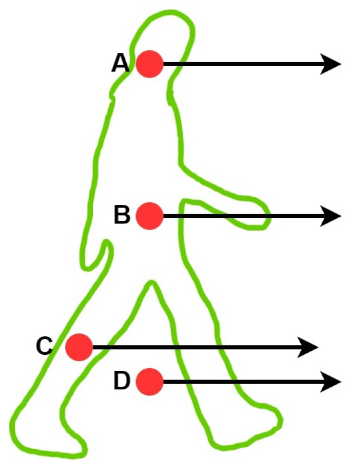
Third, we use the ray casting method to determine whether the remaining point cloud is located in the instance segment frustum region and then filter the point cloud again. The ray casting method is a detection algorithm for judging whether a point is within a polygonal area. As shown in Figure 3, a ray is emitted from any arbitrary point, thus passing through the polygonal region. If the number of intersection points within the area is even, the point is considered outside the polygonal area; if it is odd, the point is deemed inside the polygonal region.

The pseudocode of the point cloud filtering process is shown in Algorithm 1.

Algorithm 1 Mapping 3D points onto 2D plane and removing points outside the frustum

Input: 3D point cloud data: $\mathit{P}$; bounding boxes: $\mathit{Boxes}$; instance edge contours: $\mathit{Ins}$

Output: Filtered point cloud: ${\mathit{P}}_F$

1:  for each single bounding box in $\mathit{Boxes}$ do

2:        Expand box into 3D space to form frustum ${\mathit{F}}_{box}$;

3:        Perform vectorized operations using numpy to determine whether points are inside ${\mathit{F}}_{box}$;

4:        Point cloud after initial filtering is saved as ${\mathit{P}}_{F1}$;

5:  end for

6:  for each instance counter ins in Ins do

7:        Expand ins into 3D space to form frustum ${\mathit{F}}_{ins}$;

8:        for each point p in ${\mathit{P}}_{F1}$ do

9:              Use Ray Casting algorithm to determine whether p is inside ${\mathit{F}}_{ins}$;

10:              if p is inside an instance frustum ${\mathit{F}}_{ins}$ then

11:                     Add p to point cloud after second filtering ${\mathit{P}}_F$;

12:              end if

13:        end for

14:  end for

15:  return ${\mathit{P}}_F$

In summary, our algorithm facilitates both preliminary and detailed point cloud filtering. This is achieved by extending 2D bounding boxes into 3D frustums and, in the subsequent step, leveraging instance contours for further refinement. Rather than directly applying the instance contour filter to the raw point cloud, the decision to divide the filtering process into two stages is grounded in the considerable volume of points in 3D space, thereby often reaching the hundreds of thousands. The direct application of the ray casting algorithm to raw point clouds could impose undue strain on CPUs. 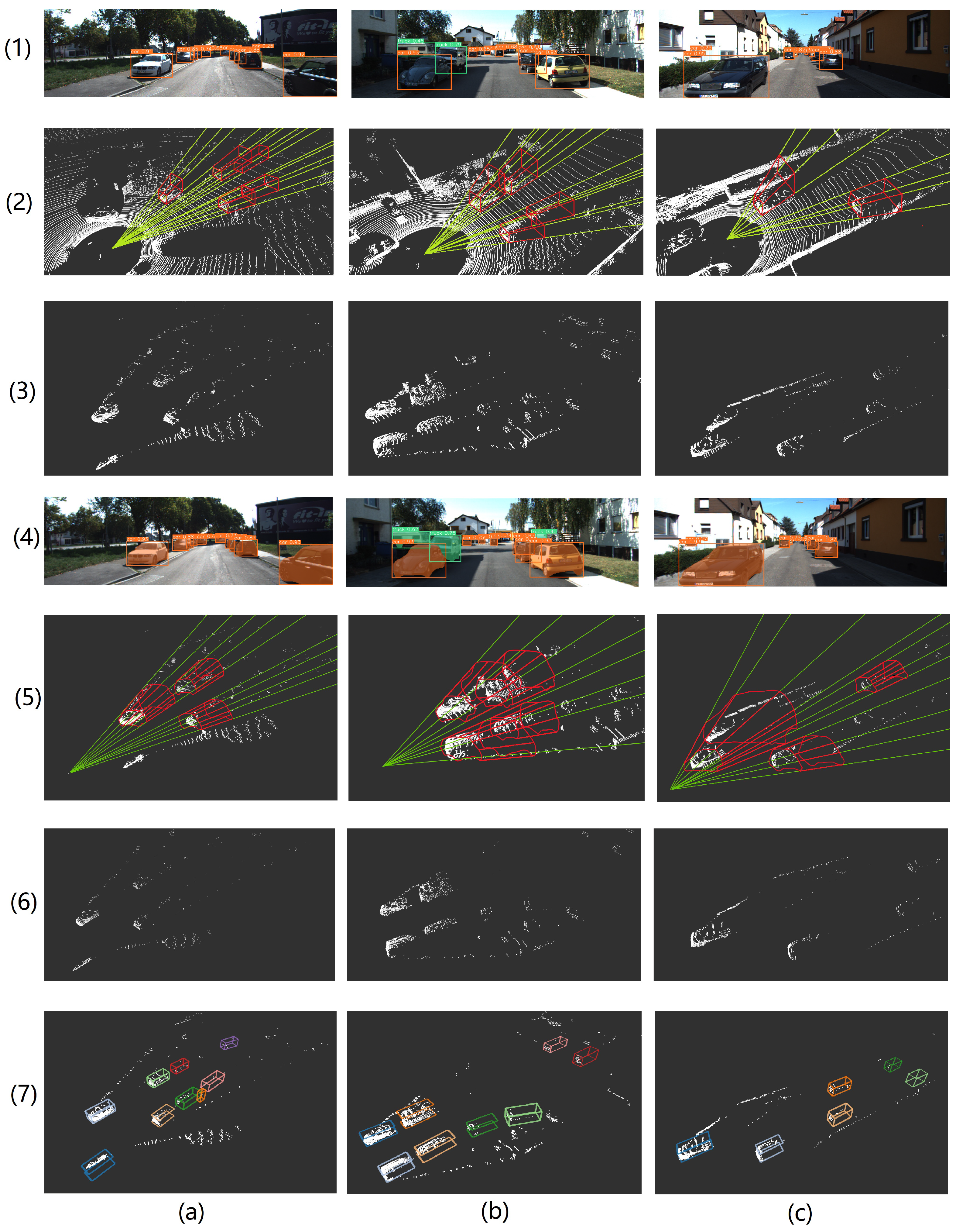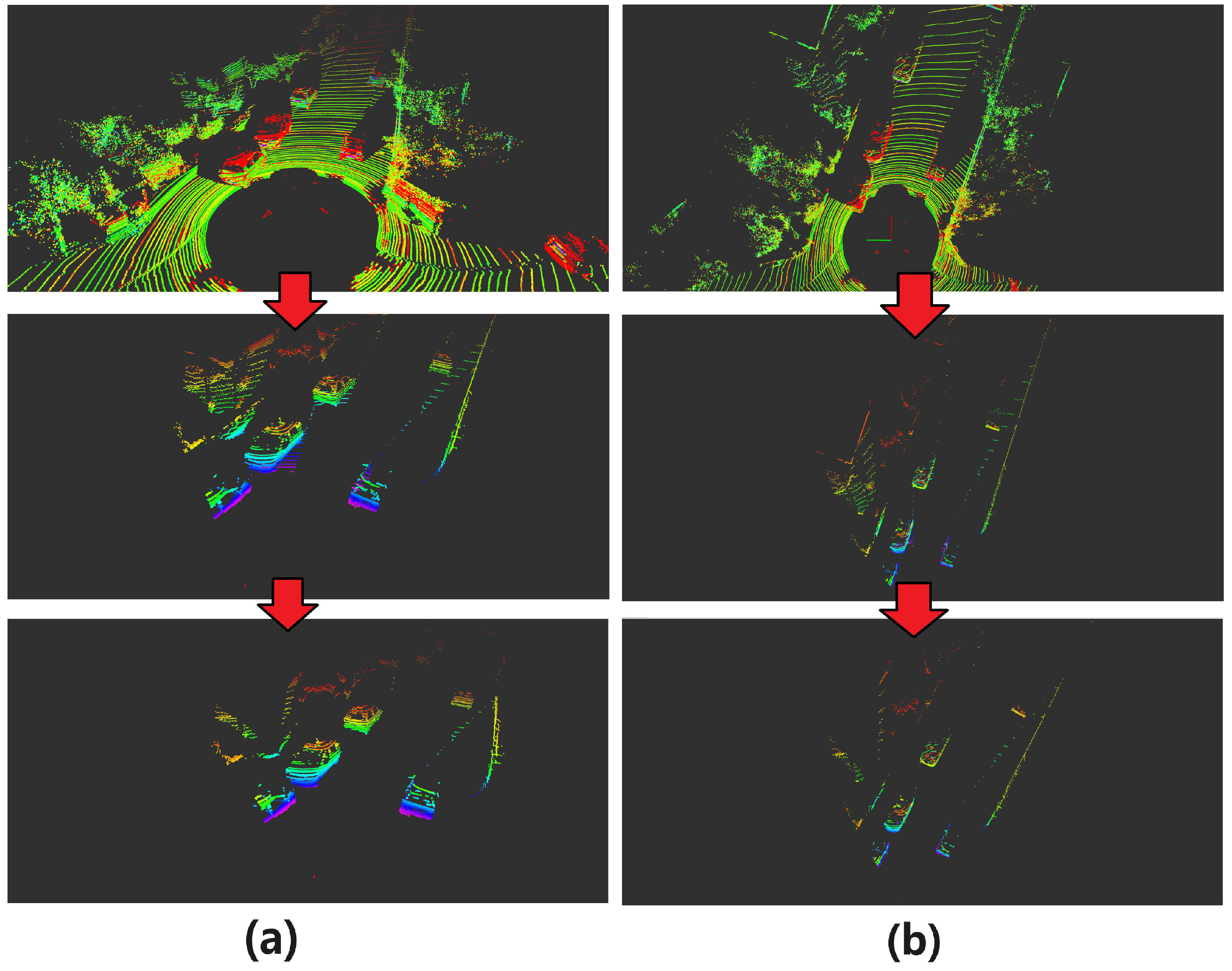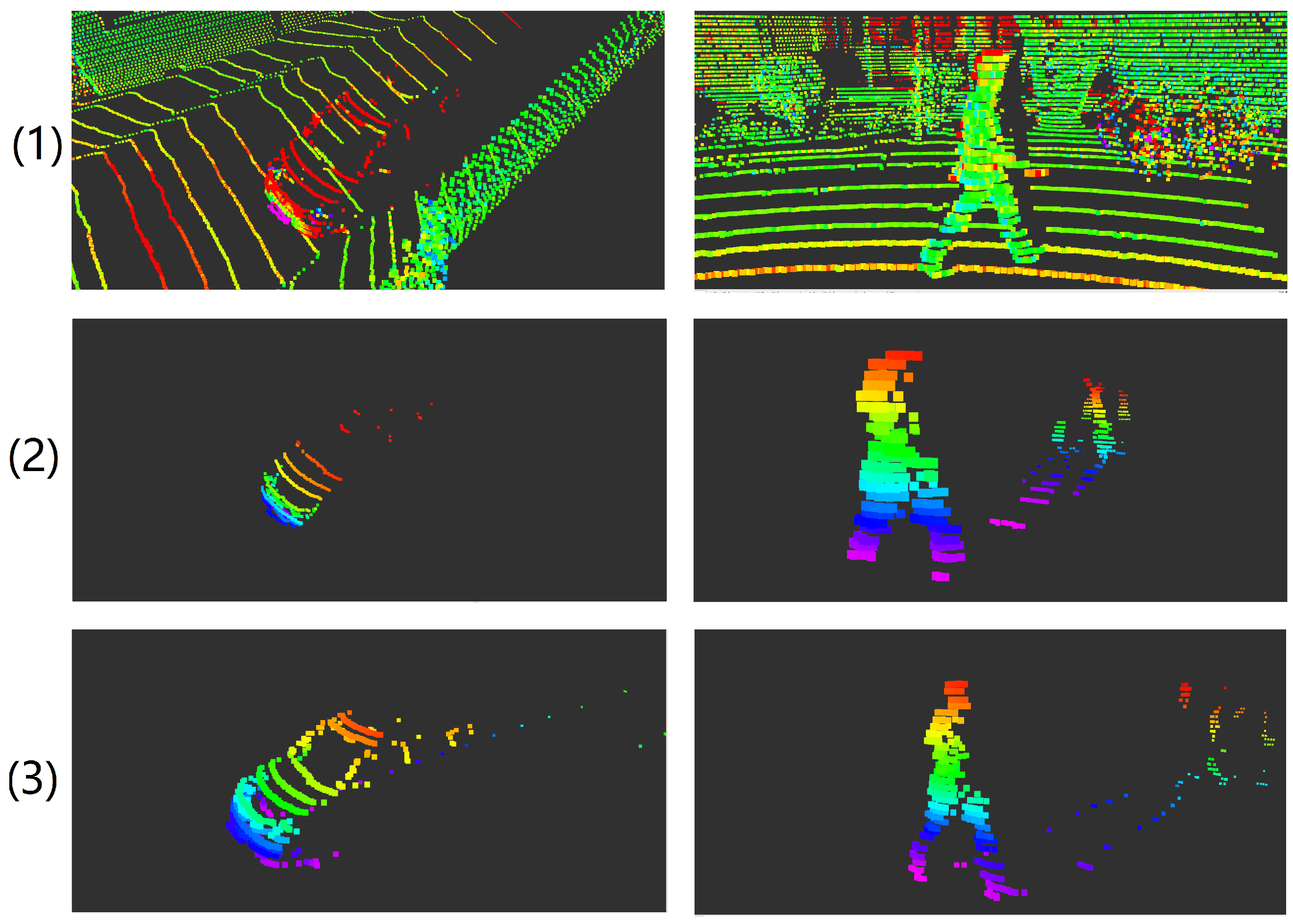Figure 4 depicts two road scenes arranged in two columns. The three rows of images correspond, from top to bottom, to the visual data of the original point cloud, the point cloud filtered via the box frustum, and the remaining point cloud filtered via the instance mask frustum, respectively. After two rounds of filtering, the background points are filtered out, and the target object points are retained.

2.2. Improving 2D Object Detection Networks

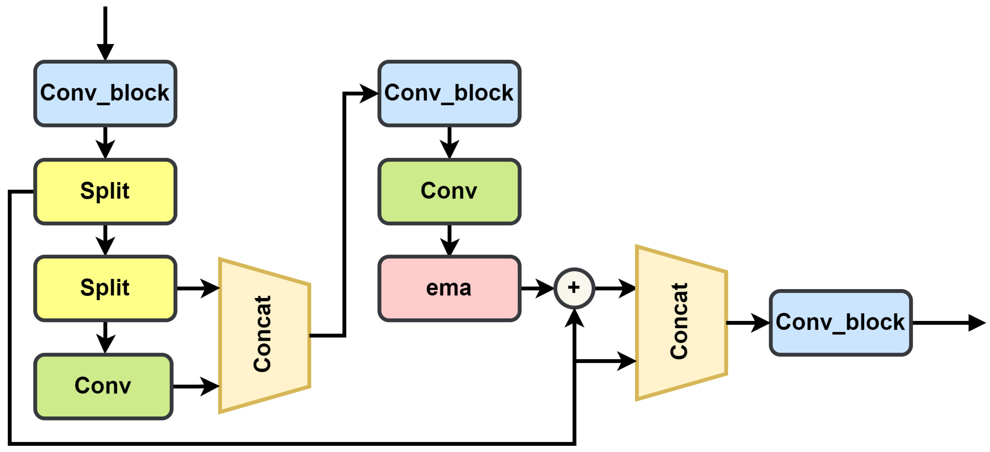
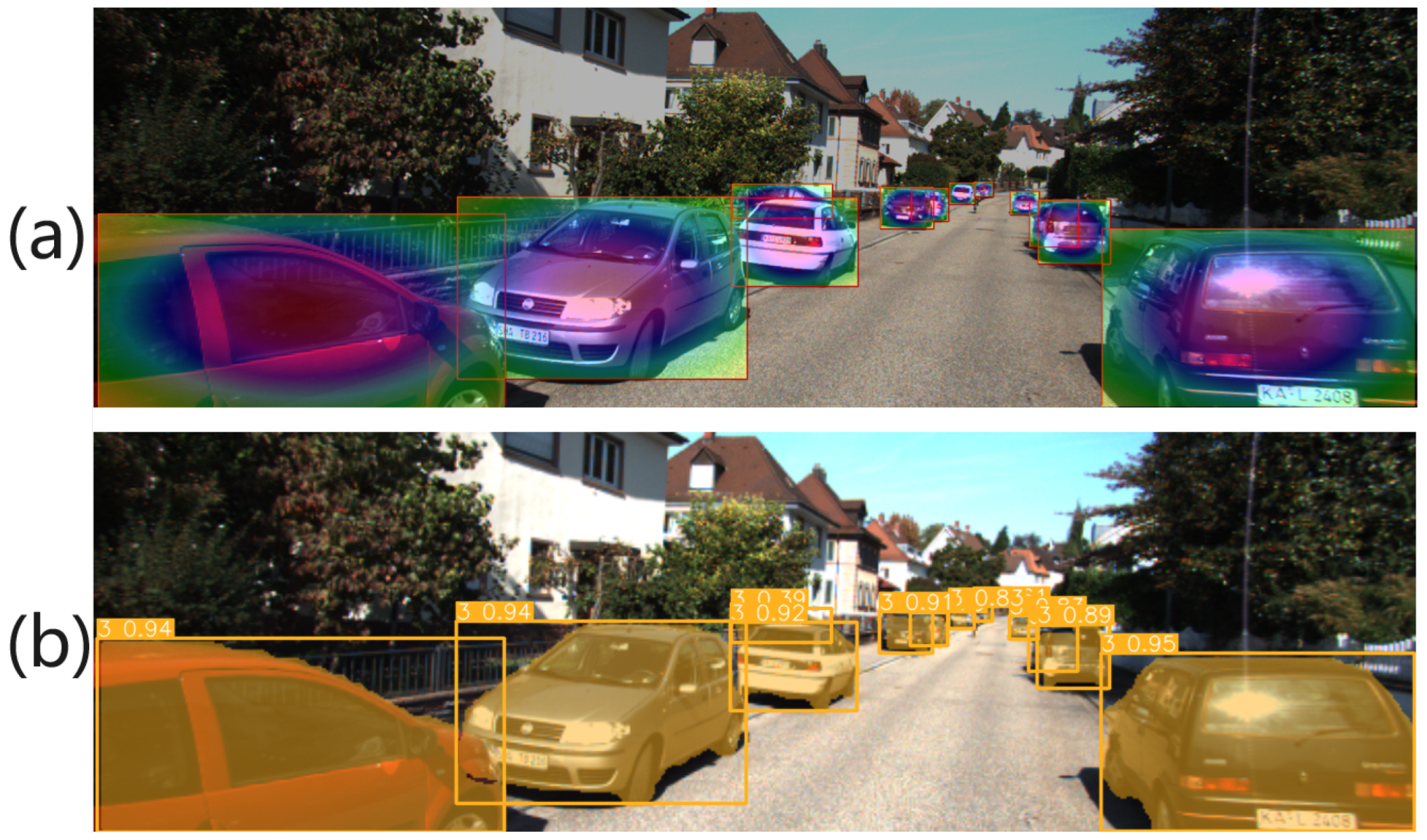
In order to improve the detection accuracy of RGB images in autonomous driving scenarios, enhance real-time performance, and reduce the amount of model calculations, we modified the 2D network. We introduced the EMA attention mechanism, which is shown in Figure 5, and the FasterNet [35] structure based on partial convolution (PConv) to reduce the number of model parameters while maintaining algorithm accuracy. These components are integrated into the C2F-FE module, as shown in Figure 6. This module replaces the C2F (the faster implementation of the cross-stage partial bottleneck with two convolutions) module in the YOLOv8 backbone. 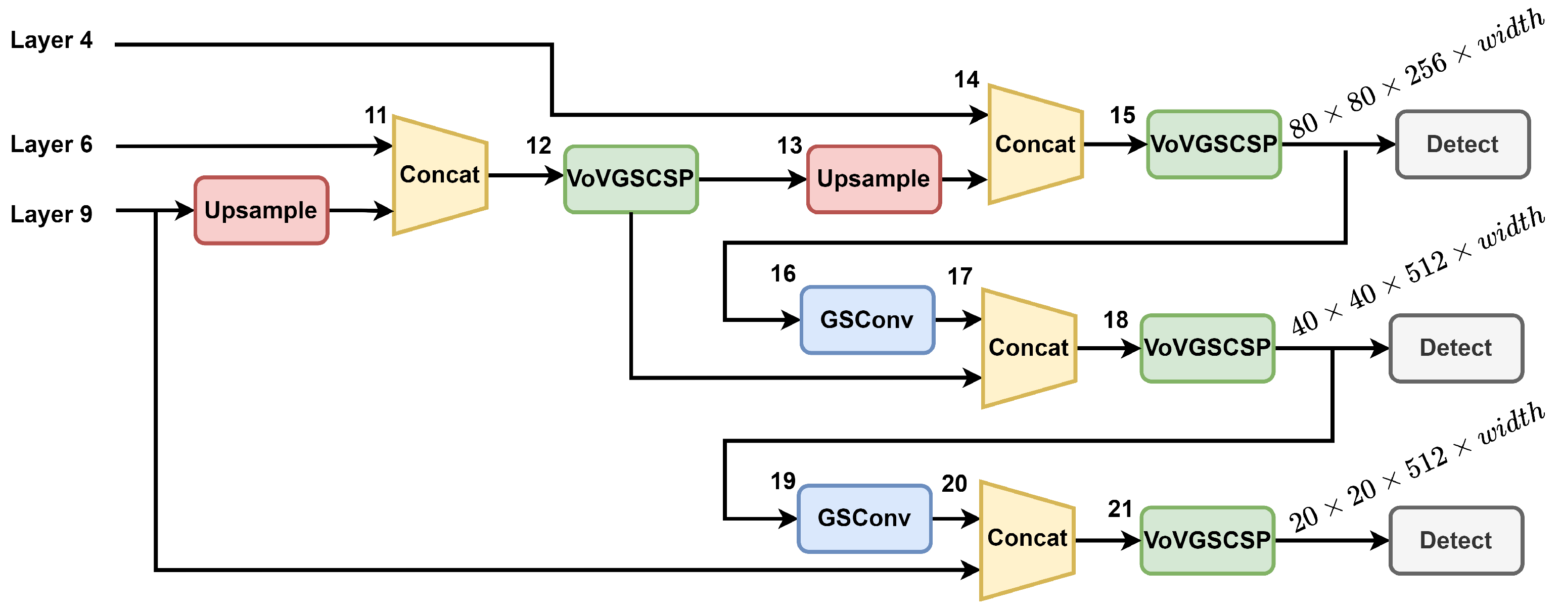Subsequently, we employed the slim-neck [36] architecture to replace the head layer, as illustrated in Figure 7.

The C2F module was extensively employed within the YOLOv8 backbone network. The C2F module design draws inspiration from the C2 module, formally known as the ‘Cross-Stage Partial (CSP) bottleneck with two convolutions’. The C2 module serves as a foundational component within the YOLOv8 architecture. C2F is an optimized version of C2 that focuses on improving execution speed without sacrificing accuracy. To further enhance the network speed, we introduced partial convolution (PConv) to more efficiently extract spatial features by reducing redundant calculations and simultaneous storage access. This improvement enhances FLOPS, boosts GPU throughput, and conserves CPU computing time.

In order to retain the information on each channel and reduce computational overhead, we introduced the EMA module and integrated it into the C2F-Faster structure, thus ultimately forming the C2F-FE module.

To further minimize the number of model parameters, we made modifications to the YOLOv8 head. We replaced the original Conv module with GSConv [36] and substituted the C2F module with VoVGSCSP [36], thereby creating a slim-neck structure.

We also adjusted the computation of the loss function. The overall loss function for 2D detection consists of three components: bounding box loss, segment loss, and classification loss. Segment loss ($L_{seg}$) uses crossentropy loss [37] to calculate instance segment loss, and the formula is as follows:

$$\begin{array}{c}\hfill L_{seg}=\frac{H_b}{\mathit{N}}·\sum _{n=1}^{n=N}(-y_n·log\left(\sigma \left(x_n\right)\right)-(1-y_n)·log(1-\sigma \left(x_n\right)))\end{array}$$

(3)

where $H_b$ represents the hyperparameters of the bounding box; N denotes the batch size; $y_n$ is the ground truth label of instance segmentation mask, which takes the value 0 or 1; $x_n$ represents the predicted instance segmentation score, with its value ranging is between $(0,1)$; and $\sigma$ indicates the sigmoid function. Classification loss ($L_{cls}$) adopts the binary crossentropy loss function.

$$\begin{array}{c}\hfill L_{cls}=-S_t·log\left(\sigma \left(S_p\right)\right)-(1-S_t)·log(1-\sigma \left(S_p\right))\end{array}$$

(4)

where $S_p$ represents the predicted value of the model, and $S_t$ represents the true value (0 or 1) of the ground truth. $\sigma$ represents the sigmoid function, thereby mapping x to the interval $(0,1)$. The computation of $L_{box}$ involves the use of the complete intersection over union (CIOU) function, which combines IoU and distance loss. The formulation is as follows:

$$\begin{array}{cc}\hfill L_{CIoU}& =1-IoU+\frac{{\rho }^2(p,p^{gt})}{c^2}+\alpha V\hfill \\ \hfill V& =\frac{4}{{\pi }^2}{\left(arctan\frac{{\omega }^{gt}}{h^{gt}}-arctan\frac{\omega }{h}\right)}^2\hfill \\ \hfill \alpha & =\left\{\begin{array}{cc}0,\hfill & \mathrm{if}\mathrm{IoU}<0.5,\hfill \\ \frac{V}{(1-IoU)+V},\hfill & \mathrm{if}\mathrm{IoU}\ge 0.5.\hfill \end{array}\right.\hfill \end{array}$$

(5)

where the CIoU computation formula involves various components. There is the IoU, which denotes the intersection over union of rectangular boxes, and it is defined as $IoU=\frac{Inter}{Union}$. The parameter $\rho$ is employed to compute the distance between the center points of the predicted box p and the ground truth box $p^{gt}$. Meanwhile, c signifies the distance between the farthest vertices of the two rectangular boxes. The parameter $\alpha$ can be tuned to facilitate the transition from CIoU to DIoU when the IoU falls below 0.5.

To quantify the extent of overlap between the bounding box and the ground truth box generated by the model, we introduced the bounding box loss function ($L_{box}$) to optimize the model’s predictive performance:

$$L_{box}=\frac{\sum (1-L_{CIoU})\times W}{\sum T_s}$$

(6)

where W is a hyperparameter used to control the weight, and $T_s$ represents the sum of confidences for all prediction results.

The distribution focal loss (DFL) function aids the network in more accurately localizing object boundaries, particularly in complex scenes:

$$\begin{array}{cc}\hfill L_{dfl}& =\frac{1}{N}\sum _{i=1}^N\left[(1-{IoU}_i)\times \left({DFL}_l+{DFL}_r\right)\right]\hfill \\ \hfill {DFL}_l& =-{\alpha }_t{(1-p_t)}^{\gamma }log\left(p_t\right)\hfill \\ \hfill {DFL}_r& =-{\alpha }_t{\left(p_t\right)}^{\gamma }log(1-p_t)\hfill \end{array}$$

(7)

where N represents the batch size, $p_t$ represents the predicted probability of the true class, ${\alpha }_t$ is a balanced parameter associated with class t, and $\gamma$ is a parameter controlling the focusing effect.

The overall loss function of the 2D object detection model is as follows:

$$\begin{array}{c}\hfill L_{total}^{2D}=L_{box}\times g_b+L_{seg}\times g_s+L_{cls}\times g_c+L_{dfl}\times g_d\end{array}$$

(8)

where the coefficient $g_b$ is the gain of bounding box loss, $g_s$ is the gain of segmentation loss, $g_c$ is the gain of classification loss, and $g_d$ is the gain of DFL loss. Adjusting these coefficients can affect the weight of each loss function in the total loss.

2.3. Three-Dimensional Detection Method

Our 3D object detection method is based on the PointPillars network. PointPillars transforms 3D point clouds into 2D BEV feature maps, as illustrated in Figure 8. First, draw a grid on the x–y plane, divide the point cloud into several pillars, and then extract features from the points in each pillar through operations such as linear, batch norm, ReLU, and max polling. All the features form a pseudoimage and are then processed via 2D CNN. This approach is distinguished by its rapid processing speed and minimal hardware requirements, thereby making it well suited for deployment in real-time detection scenarios. To further enhance the efficiency of point cloud data computation and foster seamless integration between the 3D network and the 2D detection method, we have implemented the following enhancements.

2.3.1. Encoder

The PointPillars network, implemented within the MMDetection3D [38] framework, employs PillarFeatureNet [39] to compute features for points within each voxel. Subsequently, PointPillarsScatter [24] is utilized to generate pseudoimages. To further improve the detection performance of PointPillars in autonomous driving scenarios, we made modifications. The original point cloud data include coordinates $(x,y,z)$ and LiDAR reflectivity. However, we replaced $(x,y)$ with radius, thus representing the second norm of $(x,y)$:

$$radius={\left|\right|(x,y)\left|\right|}_2$$

(9)

Since the LiDAR point cloud is annularly projected and reflects from surrounding objects with the current vehicle as the center, we combined $(x,y)$ into a variable $radius$. In this way, we can replace the original $(x,y,z,i)$ with $(r,z,i)$ to reduce data dimensionality. This operation significantly diminishes the number of computations in subsequent pipelines, thereby enhancing the overall efficiency of the algorithm.

2.3.2. Loss Function

The original PointPillars method uses focal loss to calculate classification loss, which requires presetting the hyperparameters $\alpha$ and $\gamma$ to adjust the effect of the loss function:

$$L_{cls-focal}=-\alpha {(1-p)}^{\gamma }\log p$$

(10)

However, the utilization of the weighted softmax function, with distinct weights assigned to various categories, yields improved generalization and enhanced detection performance:

$$L_{cls}=-\log \frac{w_i{e}^{p_i}}{{\sum }_j^C{w}_j{e}^{p_j}}$$

(11)

In Equation (11), $p_i$ represents the estimated probability of class i, $w_i$ signifies the weights associated with different classes, and C represents the total number of categories. Additionally, we drew inspiration from SECOND [40] for the design of the localization loss function:

$$L_{loc}=\sum SmoothL1(\Delta \mathrm{b})$$

(12)

Among them, $\mathrm{b}\in {\mathrm{R}}^3$ represents the boxes in three-dimensional space; $\Delta \mathrm{b}$ is the difference between the predicted box and the ground truth box, wherein the boxes possess attributes of $(x,y,z,w,l,h,\theta )$ that represent the three-dimensional coordinates, size, and orientation angle of the boxes; and $SmoothL1$ is a loss function used for target detection regression problems.

Finally, but equally as significant, we introduced the direction loss function to prevent 180-degree misjudgments of the target. This follows the approach used in SECOND, where softmax classification loss was also introduced:

$$L_{dir}\left(k\right)=-log\frac{e^{{\mathrm{x}}^T·{\omega }_k+b_k}}{{\sum }_{i=1}^C{e}^{{\mathrm{x}}^T·{\omega }_i+b_i}}$$

(13)

where C is the total number of categories, x is the representation vector of each sample, ${\omega }_i$ and $b_i$ represent parameters for sample x belonging to the ith class, and k represents the currently predicted category.

The final 3D target detection total loss function is as follows:

$$L_{total}^{3D}={\omega }_{cls}{L}_{cls}+{\omega }_{loc}{L}_{loc}+{\omega }_{dir}{L}_{dir}$$

(14)

where ${\omega }_{cls}$ is the weight of the classification loss function, ${\omega }_{loc}$ is the weight of the localization loss function, and ${\omega }_{dir}$ is the weight of the direction loss function.

3. Experimental Setup

3.1. Dataset and Evaluation Method

In this experiment, we employed the KITTI dataset as the benchmark for evaluation. Widely recognized in the field of autonomous driving research, the KITTI dataset encompasses a substantial collection of images, LiDAR data, and camera calibration parameters. Since the KITTI dataset does not officially disclose the ground truth of the validation set, we divided the training set. The official training dataset containing labeled samples was divided into training, validation, and testing sets using random numbers in a proportion of 7:1.5:1.5 [41].

Our detection metrics employed average precision (AP) and BEV. These two evaluation metrics consider the accuracy of target detection, directional performance, and three-dimensional spatial information, thus rendering them advantageous in autonomous driving and 3D scene understanding domains. They are crucial in comprehensively assessing target detection algorithm performance in real-world scenarios. The $AP$ calculation formula is as follows:

$$AP=\frac{1}{n_{\mathrm{pos}}}\sum _{r=1}^{n_{\mathrm{pos}}}\mathrm{Precision}\left(r\right)·\delta \left(r\right)$$

(15)

where $n_{\mathrm{pos}}$ is the total number of true positive samples, $\mathrm{Precision}\left(r\right)$ represents the precision at the rth detection, and $\delta \left(r\right)$ is an indicator function that evaluates whether the rth detection is a true positive. The computation of $\delta \left(r\right)$ is as follows:

$$\delta \left(r\right)=\left\{\begin{array}{cc}1,\hfill & \mathrm{if}\mathrm{the}r-\mathrm{th}\mathrm{detection}\mathrm{is}\mathrm{a}\mathrm{true}\mathrm{positive},\hfill \\ 0,\hfill & \mathrm{otherwise}.\hfill \end{array}\right.$$

(16)

The BEV computation can be expressed using the following formula:

$$\mathrm{BEV}(x,y)=\sum _i^N{w}_i·\delta (x_i,y_i,x,y)$$

(17)

where $\mathrm{BEV}(x,y)$ denotes the value at coordinate $(x,y)$ on the BEV grid, N represents the number of points in the point cloud, $w_i$ denotes the weight of the ith point in the point cloud, and $\delta (x_i,y_i,x,y)$ is an indicator function used to determine whether the ith point in the point cloud is projected onto the coordinate $(x,y)$ on the BEV grid. If it is, $\delta (x_i,y_i,x,y)$ equals 1; otherwise, it equals 0.

Furthermore, the KITTI dataset is stratified into three levels for all target objects—easy, moderate, and hard—corresponding to objects of varying detection difficulties. The specific division parameters are shown in

Table 1. KITTI difficulty groups.

	Max Occlusion Level	Max Truncation	Min Bbox Height
Easy	Fully visible	15%	40 Px
Moderate	Partly occluded	30%	25 Px
Hard	Difficult to see	50%	25 Px

. These three kinds of difficulties were considered in part of the controlled experiment, and the experimental results were recorded.

3.2. Implementation Details

The experiments were conducted on a computer with an Intel Xeon(R) W-2145 CPU and NVIDIA GeForce RTX 2080Ti GPU with 11 GB of memory. We chose Ubuntu 18.04.6 LTS as the operating system. The PyTorch [42] version was 1.12.0, the CUDA version was 12.0 [43], and the Python OpenCV [44] version was 4.6.0. Our 2D detection experimental code was modified based on the Ultralytics-YOLO [9] framework, and its version number is 8.0.232. The 3D object detection code was built upon the MMDetection3D framework, which is an open-source 3D object detection toolkit based on PyTorch. The software version of MMDetection3D employed is v1.2.0. MMDetection3D supports multi- and single-modal detectors, including DETR3D [45], CenterFormer [46], PointPillars, and more. This versatile toolkit provides many state-of-the-art algorithms for accurate and efficient 3D object detection tasks.

3.3. Parameter Settings

Various hyperparameters and configuration information must be initialized before training to obtain better neural network model training weights. In our experiment, the 2D network and 3D network were separately trained, each with its own set of parameter configurations.

We fine-tuned the 2D model parameters based on the outcomes of multiple training sessions. After surpassing 100 epochs, both the recall and precision parameters exhibited stagnation or a declining trend, and the loss function curve plateaued. Conversely, when the epoch was set below 100, the mAP indicator had not reached its peak. Therefore, setting the epoch to 100 was determined to be optimal. To fully leverage GPU resources and expedite training, we set the batch size to 60. The specific 2D network training parameter settings are shown in

Table 2. The 2D model parameters for training.

2D Model Paramaters
Epoch num	100
Batch size	60
Image size	640 × 640
Initial learning rate	0.01
Final learning rate	0.01
Pretrained weight	None
Optimizer	Auto
Weight_decay	0.0005
Warmup_epochs	3
Warmup_momentum	0.8
Box loss gain	7.5
Cls loss gain	0.5
Mask downsample ratio	4
Validate/test	TRUE
Masks should overlap	TRUE
Data loading threads	8
Device	2 GPUs

.

The parameter settings for our 3D object detection network are detailed in

Table 3. The 3D model parameters for training.

3D Model Paramaters
Epoch num	80
Batch size	6
Initial learning rate	0.001
Pretrained weight	TRUE
Optimizer	AdamW
Box loss gain	SmoothL1Loss
Cls loss gain	FocalLoss
Loss_dir	CrossEntropyLoss
Val_interval	2
Voxel_size	[0.16, 0.16, 4]
Point_cloud_range	[0, −39.68, −3, 69.12, 39.68, 1]
Nms_thr	0.01
Score_thr	0.1
Nms_pre	100
Device	2 GPUs

. It is important to highlight that, due to the inherent nature of the PointPillars algorithm, the choice of voxel size holds significant importance. A large voxel size may lead to information loss, while an excessively small voxel size could substantially increase computational demands. Given the unique characteristics of different LiDAR systems, it becomes imperative to make tailored adaptations based on the specific circumstances and characteristics of the LiDAR sensor in use.

4. Experimental Results

This section describes the experimental results of the Instance Segmentation Frustum–PointPillars method on the KITTI dataset. The visual data output at each stage during the algorithm processing is shown in Figure A1.

4.1. Results on KITTI Dataset

Accuracy

Our algorithm was compared with the mainstream 3D object detection algorithm on the KITTI dataset. We set up controlled experiments to compare our method with existing mainstream 3D object detection methods for the car and pedestrian categories in the KITTI dataset. The experimental results show that the AP index of methods based on the fusion of camera and LiDAR (such as F-PointPillars and F-ConvNet) was overall better than methods that rely only on LiDAR (such as Second and Voxelnet). Our method outperformed similar fusion algorithms in this experiment. The specific results are shown in

Table 4. The 3D average precision.

Method	Car			Ped.
	Easy	Moderate	Hard	Easy	Moderate	Hard
Second [40]	88.36	78.22	76.03	67.44	65.91	63.22
Voxelnet [47]	81.97	65.46	62.85	39.48	33.69	31.51
PointPillars [24]	87.84	77.63	75.95	62.57	57.52	51.17
F-PointNets [30]	83.76	70.92	63.65	70.00	61.32	53.59
F-ConvNet [31]	89.31	79.08	77.17	52.16	43.38	38.08
F-PointPillars [32]	88.90	79.28	78.07	66.11	61.89	56.91
Ours	88.94	79.65	78.04	67.45	66.84	61.94
Task	3D object detection

. The bold numbers within the table indicate the highest value within each column.

Similar to the abovementioned experiment, we conducted another BEV indicator test. A visual result of BEV detection is shown in Figure 9. When comparing the experimental results, our method improved the detection accuracy of pedestrians. In the easy and moderate difficulty levels, our detection accuracy for cars led the comparison, only slightly trailing behind F-PointPillars in the hard level. Detailed results are shown in

Table 5. BEV accuracy.

Method	Car			Ped.
	Easy	Moderate	Hard	Easy	Moderate	Hard
Second [40]	89.97	87.23	84.31	67.14	67.00	64.17
Voxelnet [47]	89.60	84.81	78.57	65.95	61.05	56.98
PointPillars [24]	89.99	87.13	85.15	70.54	65.70	60.18
F-PointNets [30]	88.16	84.02	76.44	72.38	66.39	59.57
F-ConvNet [31]	90.42	88.99	86.88	57.04	48.96	44.33
F-PointPillars [32]	90.20	89.43	88.77	72.17	67.89	63.46
Ours	90.89	90.68	88.17	75.17	69.05	64.99
Task	BEV

.

We scrutinized the aforementioned experimental outcomes and deduced the factors contributing to the suboptimal performance of our algorithm in the “hard” category. First, model design plays a crucial role; while using instance segmentation masks instead of Gaussian masks can accurately differentiate foreground and background points in 3D point clouds, this approach may encounter challenges in handling complex scenes. For instance, in “hard” level scenarios, targets may be obscured by other objects, shadows, or blend into the background, thus potentially impacting the effectiveness of instance segmentation masks. Second, training strategies significantly influence performance. The choice of loss functions, optimizer settings, data augmentation methods, etc., can shape its performance. To maintain a balance in the overall performance of our algorithm, optimization was not specifically tailored for the relatively small proportion of scenarios in the “hard” level. Third, dataset characteristics are vital. Characteristics such as sample distribution and annotation accuracy play a role in influencing the model’s performance. Given the smaller proportion of “hard” level samples in the dataset and the potential noise in annotations for these samples, the model’s performance at this level might be affected.

4.2. Ablation Study

4.2.1. Effect of Point Filter

We conducted several experiments to validate the effectiveness of the point filter algorithm proposed in this study. After filtering a substantial number of original LiDAR 3D points through the box frustum and instance mask frustum, the point count was markedly reduced, thus conserving processor resources and enhancing data processing speed. Numerous experiments were conducted on the KITTI dataset, and the comparative experimental results are presented in

Table 6. A comparison of the number of remaining points after processing using different methods.

	Point Number	Data Size/Byte
Raw Points	118,662	1,898,576
Box Frustum Filtered	6641	106,240
Gauss Mask Filtered	5967	95,458
Instance Mask Frustum Filtered	4658	74,512

.

In addition, we observed that precise point cloud filtering contributed to an improvement in the accuracy of subsequent 3D target detection. The results are shown in

Table 7. Accurate segmentation algorithm improved BEV accuracy.

Method	Car			Ped.
	Easy	Moderate	Hard	Easy	Moderate	Hard
PointPillars	89.99	87.13	85.15	70.54	65.70	60.18
PointPillars and Box Frustum	90.20	89.43	88.77	72.17	67.89	63.46
PointPillars and Gaussian Frustum	90.16	89.25	87.64	73.12	66.54	64.88
PointPillars and Instance Mask Frustum	90.89	90.68	88.17	75.17	69.05	64.99
Task	BEV

.

Compared to generating boundaries using a Gaussian-based approach, as utilized in F-PointPillars, our method allows for a more accurate separation of the foreground and background points, as shown in Figure 10. In Figure 11, we present a comparative analysis of the efficacy between Gaussian distance-based and instance segmentation-based methods for delineating the boundary contours of target objects within bounding boxes. In Figure 11a, regions with darker colors indicate smaller Gaussian distances, thus signifying a heightened likelihood of association with the target object. The Gaussian-based approach employs a distance threshold to distinguish target objects from extraneous elements. Figure 11b demonstrates the application of the instance segmentation method, thereby enabling pixel-level accurate segmentation of both the target objects and background. This approach significantly enhanced the precision compared to the methodology employed in Figure 11a. Furthermore, we maximally preserved the shapes and details of objects, thus avoiding unnecessary data loss or blurring, which makes it more suitable for processing point cloud data with complex shapes and topological structures. Additionally, point clouds filtered through the instance segmentation method typically have fewer points than those separated using the Gaussian-based method. This ensures a faster processing speed when handling large-scale point cloud data via 3D object detection networks. Furthermore, instance segmentation enhances the understanding of object instances within the point cloud, thereby enabling individual treatment for each instance and ensuring independent processing for every object. This helps prevent mutual interference between instances, thus enhancing the inference effect. As a result, using 2D instance segmentation masks to generate frustums for point cloud filtering led to superior performance compared to the Gaussian-based method.

4.2.2. Improvements on 2D Detection

To validate the enhancement achieved using our 2D model, we compared the detection performance of the YOLOv8 instance segmentation model on autonomous driving scene datasets before and after incorporating the C2F-FE module. The results, as shown in

Table 8. Comparison of 2D detection algorithms on the car category in the KITTI dataset.

Model	Class	Precision	Recall	mAP50	mAP50-95	Time (ms)
Mask R-CNN [5]	Car	0.546	0.434	33.1	32.7	8.4
YOLOv5 [19]	Car	0.544	0.445	33.4	30.2	8.7
YOLOv8 [9]	Car	0.563	0.449	33.9	30.5	8.5
YOLOv8 and C2F_FE	Car	0.581	0.454	35.6	32.4	6.7
YOLOv8 and slim-neck	Car	0.572	0.450	34.0	32.6	8.1
Ours	Car	0.584	0.459	35.9	33.0	7.0

and

Table 9. Comparison of 2D detection algorithms on the pedestrian (Ped) category in the KITTI dataset.

Model	Class	Precision	Recall	mAP50	mAP50-95	Time (ms)
Mask R-CNN [5]	Ped	0.549	0.270	32.9	31.6	8.3
YOLOv5 [19]	Ped	0.550	0.264	32.4	32.0	9.2
YOLOv8 [9]	Ped	0.556	0.267	32.6	31.2	9.1
YOLOv8 and C2F_FE	Ped	0.562	0.271	34.7	33.9	7.8
YOLOv8 and slim-neck	Ped	0.554	0.269	34.5	33.7	7.9
Ours	Ped	0.568	0.274	34.7	33.7	7.7

, indicate that our improvements to the backbone network demonstrated increased speed while ensuring accuracy. Furthermore, we also confirm that the slim-neck structure enhanced the detection performance of YOLOv8.

The detection results for the KITTI RGB images are shown in Figure 12. Our instance segmentation mask was more accurate than the original YOLOv8 model, which could improve the accuracy of the point cloud filtering. The tables and figures above show that optimizing the backbone of YOLOv8 by replacing the C2F module with the C2F-FE module can significantly reduce inference time. In addition, the detection accuracy can be further improved by using the slim-neck structure to improve the head.

5. Conclusions

This research proposed a camera and LiDAR fusion perception method called ISF–PointPillars, which can accelerate the implementation of fusion algorithms in autonomous driving. This research included the study of the background point filtering algorithm, the modification of the 2D target detection network, and the optimization of the 3D target detection network.

Firstly, the RGB image data were processed via our enhanced 2D target detection network based on YOLOv8. This processing yielded rectangular frames outlining obstacles, including cars, pedestrians, and bicycles, along with instance segmentation edge points. Secondly, LiDAR was used to collect the 3D point cloud of the road environment; then, its spatial coordinate correspondence with the RGB image was established. Subsequently, the rectangular frames and instance segmentation edges generated via the 2D detection network were extended into 3D space to create a frustum. Only the 3D points within the frustum were retained, thus effectively eliminating invalid background and ground points. Finally, the remaining points were sent to the 3D target detection neural network for processing to obtain the coordinate, category, size, and other information about the obstacles. This approach allows us to tackle the complexities of 3D object detection in point clouds, especially in scenarios where multiple sensors are used. By integrating camera and LiDAR data, we demonstrated improved performance and accuracy, thereby making significant advancements in multisensor fusion for 3D object detection. Our proposed methodology holds promising potential for various applications, including autonomous driving platforms, robotics, and augmented reality systems.

In the future, we will focus on optimizing the detection accuracy of cyclists in BEV and average orientation similarity (AOS). We are also committed to further optimizing the 2D instance segmentation model to enhance the detection accuracy, particularly for the “hard” category in 3D object detection. Additionally, we aim to streamline the instance segmentation method for occluded objects to tap into the full potential of this algorithm.