1. Introduction
Distributed-power-generating sources (DPGSs) have created a paradigm contrasting the conventional power system. The sources have paved the way for a technology suitable for electricity generation in a limited capacity that is located near the point of consumption. The specific definition and implementation of DPGSs can vary significantly from one country to another and even within regions of the same country [
1]. This variation is due to several factors, including differences in available renewable and other energy resources, the grid infrastructure, government policies, and local energy demands. The diversity in the definitions and approaches to DPGS reflects the adaptability of this concept to the unique needs and circumstances of different countries and regions, making it a flexible solution for addressing various energy challenges [
2]. Generally, DPGS technologies can be categorized based on the devices and fuels utilized, broadly encompassing generators and storage systems. The majority of these systems can produce both active and reactive power, although their capabilities vary significantly from one another. A detailed technical overview and analysis are presented for each DPGS technology in [
1]. Many of these technologies harness energy resources, characterized as sources typically resistant to depletion. These encompass solar radiation, wind, biomass, hydropower, marine energy, and geothermal sources [
3]. Few other technologies, including small-scale hydroelectric systems, photovoltaic arrays, diesel and wind generators, solar–thermal units, fuel cells, and battery storage technologies, comprise numerous small modules assembled in factories. These technologies’ manufacturing and on-site construction need considerably less time than the process for large centralized power stations [
4].
As the popularity and integration of DPGSs continue to grow, it has become essential to develop and implement standards that ensure interoperability, efficiency, and safety across these distributed resources [
5]. Several standard organizations [
6] have emerged to address this need and have developed various standards related to DPGSs. One of the notable standard organizations in this field is the International Electrotechnical Commission (IEC) [
7]. The IEC has published several standards relevant to DPGSs, including IEC 61850, a communication standard for intelligent electronic devices used in power substations. This standard enables the exchange of information between different DPGSs and facilitates their integration into the grid.
Similarly, the IEEE [
8] has also developed several standards related to DPGSs. IEEE 1547 is a widely recognized standard that defines the interconnection requirements for DPGSs with the electric power system. It specifies the technical and operational requirements for a reliable, secure grid integration interfaced with DPGSs. Moreover, the National Electrical Manufacturers Association (NEMA) has developed the NEMA SG 4 standard, providing guidelines for evaluating, selecting, and integrating storage energy systems into electrical systems. There are also regional and national standards specific to certain countries or regions. For instance, in the United States, the Smart Grid Interoperability Panel (SGIP) has developed standards and guidelines for energy resource integration, including the Open Field Message Bus (OpenFMB) standard, which enables interoperability between different DPGSs. When comparing these standards, it is imperative to consider factors such as scope, applicability, and adoption. Some standards may have a broader scope, covering multiple aspects of DPGS integration, while others may focus on specific technologies or applications.
The adoption and implementation level of the above standards also varies across different regions and countries. Overall, the analysis and comparison of these standards help stakeholders in the energy sector understand the requirements and best practices for integrating DPGSs into the grid [
9]. These standards play a vital role in successfully deploying distributed energy resources worldwide by promoting interoperability, efficiency, and safety. An overview of varied distributed-power-generating source technologies has been presented by authors in [
10]. The study gave an insight into the environmental impacts of DPGSs over conventional-power-generating sources. Studies on DPGSs, such as wind turbines and PV panels, have revealed the positive and negative effects on power systems in recent years. While DPGSs contribute to renewable energy integration and reduce greenhouse gas emissions, their increased penetration levels can pose challenges to the power grid’s reliability and stability [
11]. Some adverse impacts associated with high levels of distributed generation include frequency and voltage instability, the reduction of the transient stability margin, protection co-ordination challenges, and grid imbalance [
12].
In a distribution system, electricity is typically transmitted to substations through high-voltage transmission lines, thereafter lowering the voltage and distributing it to homes, businesses, and other consumers. Distributed-power-generating sources are connected to the transmission system and can help meet the local load demand without requiring extensive transmission and distribution infrastructure.
Integrating DPGSs into the transmission system offers the following technical and operational advantages [
13]:
Decreased line losses and improved voltage profile: DPGS systems located closer to the load reduce the distance electricity travels, minimize transmission losses, and help maintain a stable voltage level in the transmission system. In addition, lower costs for system operation and its maintenance, associated with reduced transmission losses, contribute to cost savings for utilities.
Enhanced stability and power quality: DPGS systems can provide local stability, ensuring a consistent power supply and improving the overall quality of electricity.
Increased network efficiency and reliability: DPGS integration optimizes the utilization of existing infrastructure, making the system more efficient. Moreover, by providing backup power during grid outages, DPGS systems can enhance reliability.
Security enhancement: Distributed generation can enhance the security of the electricity supply by reducing the dependence on centralized power plants, making the system less vulnerable to large-scale failures or attacks.
Reduced transmission and distribution (T&D) congestion: By generating power closer to the point of consumption, the DPGS mitigates congestion issues by reducing the strain on T&D lines.
Delayed investments for upgrading facility: Integrating DPGSs can defer the necessity for significant investments in new T&D infrastructure, saving costs for utility companies.
Suppression of fuel costs for distributed energy resources: Renewable energy sources used in DPGS (wind/solar) systems have no fuel costs, making them economically attractive and environmentally friendly alternatives to traditional fossil-fuel-based generation.
In addition to the above, integrating DPGSs into the transmission system offers economic advantages by reducing costs, creating revenue streams, providing environmental benefits, lowering emissions, and improving air quality. Further, the operational improvements in grid reliability and stability contribute to long-term sustainability by diversifying energy resources and promoting renewable energy adoption [
14]. With the advent of several technologies contributing to the advantages mentioned above, however, stability is one of the major concerns when DPGSs are integrated into the transmission system. Researchers and industry professionals are focusing on developing advanced monitoring, control, and mitigation strategies to maintain the stability and resilience of transmission systems in the face of these evolving demands and challenges [
15].
The present work investigates the transmission system stability when power demand increases in terms of induction motor load at the load centre interfaced with DPGSs. Hence, the following section presents previous studies focusing on the impact and evaluation of power system stability with DPGSs.
2. Literature Review
At various stages of research, researchers have investigated the impact of interfacing DPGSs on the stability aspects by employing different types of DPGS technologies in a power system that includes synchronous generator-based power-generating sources, renewable- and non-renewable-power-generating technologies, and sources interfaced with power converters (like a wind turbine, photovoltaics, fuel-cell, and gas- and microturbine-power-generating sources).
In [
16], the authors examined the influence of a synchronous generator interfaced with a small hydropower-generating source of a Brazilian power grid by analyzing the stability aspects of the system. The study unveiled an improved voltage stability margin and transfer capacity due to increased power-generating source levels. A corresponding investigation involving synchronous-generator-based-power-generating sources in the distribution network is carried out in [
17]. A technique based on projective integration is applied for rapidly simulating transient stability, particularly in the presence of the high penetration of distributed-power-generating sources and virtual synchronous generators [
18]. Few other researchers [
19] have emphasized the study of synchronous and asynchronous generator-based distributed-power-generating source technology. The study focuses on the distinct characteristics of these technologies and their impact on the stability of the power grid. The authors in [
20] simulated various fault conditions to demonstrate the effect of DPGSs on transmission system transient stability. The study analyzed different fault scenarios occurring in multiple branches of the system, considering N-1 security to assess the system’s robustness.
A detailed survey was carried out to analyze the behavior of voltage variation in a DPGS-interfaced distribution network [
21,
22]. In [
23], the influence of system parameters on voltage oscillations is examined with the aid of participation factors and eigenvalues. Several researchers have suggested a number of techniques to analyze the voltage stability of the system. In [
24], an extensive voltage profile study is carried out under the influence of different power-generating sources. The study revealed that a power system under stress undergoes voltage instability, frequently due to the increased load demand at a particular bus. The authors [
25] formulated an analytical approach to enhance the reliability and voltage profile by strategically placing and sizing the renewable generating sources on distribution systems. Subsequently, various intelligent methods have also been reported due to the potential benefits of installing DPGSs on the distribution network [
26].
In [
27], the transient stability was analyzed by studying a hybrid system incorporating various renewable power generation sources. The authors concluded that the influence of power generation sources is contingent on both its location and type. Furthermore, the authors reported that stability declined as the penetration level of power-generating sources increased. In [
28], authors have proposed an optimal algorithm to control the frequency in a hybrid system and co-ordinate between various power-generating sources.
A comprehensive mathematical model and several simplified versions of the microturbine power-generating sources that utilize liquid and gas fuel systems were detailed in [
29]. Apart from the study in [
30] focusing on the system’s transient response, a comprehensive investigation on small-signal stability incorporated a microturbine power-generating source. The analysis indicated that transient stability is enhanced with increasing DPGS penetration levels, whereas the excitation control parameters of the power-generating source influence the small-signal stability. In [
31], authors investigated the small-signal and transient stability in a transmission system with rotating types (such as micr-turbine, diesel turbine, and wind turbine generators) of DPGSs interfaced at the load buses. The study revealed that the system’s stability will be degraded when DPGS penetration exceeds a certain optimum level. Moreover, the study in [
32] showed that the stability performance under the unequal load increase condition differs considerably compared to the equal load increase condition even for the same DPGS penetration level.
An extensive study on dynamic voltage stability is carried out on a hybrid system comprising conventional- and renewable-power-generating sources [
33]. This study presented a comparative analysis involving various types of static VAR compensators, utilizing minimum first swing and damping associated with subsequent oscillations as indicators. Authors in [
34] analyzed the small-signal stability of a distribution system interfaced with renewable-power-generating sources. In this study, the authors employed supplementary controllers to improve the damping ratio of critical modes. Furthermore, the study reported substantial involvement of both induction and synchronous generators in the oscillating modes.
Apart from the integration of DPGSs, researchers have been investigating the influence of dynamic loads on the distribution system [
35]. These studies aim to understand and address the challenges posed by dynamic loads separately from other types of loads [
36]. The studies in [
37,
38] reported the influence of dynamic loads on short- and long-term voltage stability.
In recent years, DPGS technologies have received significant interest in smart grids, microgrids, and distribution network applications [
39]. Although this technology focused on improving efficiency, reliability, and sustainability, many investigations have reported specific technological issues concerning DPGSs and their operation. Researchers in [
40] have analyzed the stability aspects considering the interaction between the dynamics of DPGSs with constant power loads. A study based on techniques of synchronization [
41] to extract positive–negative sequence components under the influence of inverter-based DPGSs is performed under varied grid conditions.
Some of the significant issues that have been identified based on the literature review are summarized below:
Most of the earlier findings reported the influence of DPGS penetration on system stability as applied to distribution networks. However, the latest articles have focused on installing DPGSs either at the load centres or distribution substations of transmission networks to meet any growth in load demand in the near future;
Most of the stability studies reported are in the area of microgrids, focusing on analyzing the influence of constant power loads with interfaced DPGSs;
In most articles, researchers have focused more on analyzing the effect of increased constant power loads in a transmission/distribution network interfaced with DPGSs. Therefore, it is essential to examine the dynamic load influence in a transmission/distribution network;
Across a spectrum of research publications, the emphasis is on analyzing the influence of DPGSs on transient or voltage stability. Conversely, the impact of DPGS penetration subjected to small disturbance conditions needs to be explored.
Inspired by the aforementioned requirements, the paper’s key contributions include:
Analyzing the transmission system stability when the DPGS supply increased power demand, comprising both constant power and dynamic loads;
Investigating the influence of constant power and dynamic loads on a system’s small-signal stability with the aid of the critical damping ratio and electromechanical mode eigenvalue analysis;
To study the impact of both dynamic and constant power load changes on the transient stability of the system and to further quantify the transient performance of DPGSs using time-domain indicators;
To employ the variance analysis test to determine the relative contribution of various control factors on the variance of system response.
3. Transmission System Modelling
3.1. Model of DPGS-Interfaced Transmission System and Induction Motor Penetration Level
Figure 1 illustrates the DPGS-interfaced transmission system model employed in the present study. In this model, the DPGS is interfaced at a load bus so that the increased load demand at this bus is directly supplied by the interfaced DPGS. The central concept of this model is to locally deliver the increased load demand at a load centre by a DPGS so that the power generation of main generating stations and the line power flow in the transmission system remain almost unaffected.
In the model of
Figure 1,
PLk and
QLk are the base real and reactive power demand at load bus
k. If Δ
PLk is the increase in the load real power at bus
k, then the real power generation of the interfaced DPGS is set as
PDG = Δ
PLk.
In the present study, the increased power demand ΔPLk at load bus k is assumed to have the following two parts:
A portion, (ΔPCP)k, is the increased CP demand;
The remaining portion, (ΔPIM)k = ΔPLk − (ΔPCP)k is due to the increased power demand in the form of an induction motor.
The above load demand increase model will enable the study of the effect of induction motor loads on the stability of the transmission system interfaced with a DPGS.
The constant power load change and the induction motor load are expressed as a fraction of base real power load demand at bus
k, and are defined as:
Hence, the net load power change at bus
k is given as:
The degree of the induction motor penetration level (
IMPL) is the ratio of the net induction motor load to the net real power demand of the system and is given by:
where
PLoad is the net base real power demand of the transmission system.
3.2. Transmission System and Distributed Power Generation Models
The various assumptions made while modeling the entire system are as follows:
The power system is modeled by employing all synchronous generators by fourth-order model-1.1 (d-q axis model), operated by a static exciter (IEEE type-ST1 single time-constant model, automatic voltage regulator with time-constant TE = 0.05 s and gain KE = 50);
A speed-based, two-stage lag-lead-type power system stabilizer (fixed structures PSS) and a simplified model of a steam turbine for main synchronous generators [
42] are used;
A constant impedance representation of all constant power loads is used during the simulation process.
All the dynamic equations of the synchronous generator are provided in
Appendix A.
3.2.1. Induction Generator Model
In the present study, a third order model of IM is employed [
43]. This model assumes that the rotor dynamics are slower than stator flux transients. The IM state equations are given as:
The complex voltage behind transient reactance and the motor terminal voltage relationship is given by:
In Equations (6) and (7),
is the transient open-circuit time constant;
is the transient reactance;
is the rotor open-circuit reactance.
3.2.2. Distributed-Power-Generating Sources
The following synchronous-generator-interfaced DPGSs are employed in the investigation:
The microturbine is the prime mover for a synchronous generator for a MTGS and
Figure 2 shows the general model. The MTGS is primarily based on the gas turbine model and was used in many past studies [
44,
45,
46].
The MTGS prime-mover consists of a compressor, combustor, and turbine, which drives a synchronous generator; the transfer function model of the MTGS is depicted in
Figure 3. The speed controller associated with the microturbine is operated in the isochronous mode. In the isochronous mode, the rate of change of the speed controller output varies proportional to the speed error input of the connected PI controller so that the generator maintains its speed even under load changes. The speed governor transfer function has gain
KW and governor time constants
Tx and
Ty.
The main dynamic component of the MTGS is the compressor turbine modeled by a first-order transfer function with time constant
Tcd. Due to the associated compressor discharge volume, the compressor output cannot respond instantaneously to any changes in its input. The combustor time constant
Tecr is a small value related to the combustion reaction. The fuel system comprises a valve positioner and an actuator; the inertia of both governs the dynamics of the entire fuel flow mechanism. In the MTGS model of
Figure 3,
Wmin is the minimum fuel flow, whereas
Kf and
Ka are the fuel system feedback and gain of valve positioner, respectively. The mechanical torque output of the turbine is expressed by a function
Tmt and is given by:
where
is the electrical rotor speed.
A DTGS comprises a synchronous generator driven by a diesel turbine prime mover; the general block diagram of the DTGS model is shown in
Figure 4 and consists of an electric control box, actuator, and IC engine.
A diesel turbine uses liquid fuel or natural gas as the primary fuel and operates on air compression and fuel. Initially, the air is blown into the engine until it is compressed and then the fuel is injected to generate the heat, which triggers the fuel inflammation.
Figure 5 depicts the simplified transfer function model of the DTGS, representing the essential dynamics and is adapted from [
44,
47]. The main processes accounted for in this model are the (i) fuelling actuation, (ii) combustion or torque production, and (iii) crankshaft torque balance of the engine. The time delay between the fuel-flow actuation and subsequent power stroke is represented by the time constant
TDd.
4. Problem Formulation and Solution Methodology
The influence of induction motor loads on the small-signal stability of the transmission system interfaced with a DPGS is studied using eigenvalue analysis and the critical damping ratio (
ζcr) of oscillating mode eigenvalues. The linearized state-space model of the system at an initial operating point assuming constant inputs can be formulated as:
In Equation (10),
ΔX is the vector of state variables, and
A is the state matrix. The state matrix
A can be used to determine the system’s eigenvalues for specified system parameters and operating state. Considering a complex conjugate (oscillating mode) eigenvalue
, the associated damping ratio can be determined as:
The critical damping ratio is the minimum of the damping ratio associated with oscillating mode eigenvalues, given as:
The transient performance of the transmission system with a DPGS and supplying IM loads is analyzed by simulating self-clearing faults of duration tc seconds on the mid-point of a transmission line. The following time-domain indicators are used to quantify the transient performance:
Maximum slip deviation (MSD): the maximum slip deviation among relative slip response generators. It indicates the worst value of peak responses;
Settling time (ST): the maximum settling time among the relative slip deviation responses of generators, measured with a 2% tolerance band.
The present study performs all the simulations using Simulink/Matlab software (version 7.1, R14) [
48]. In the approach, the solution of the differential equations of all system components is modeled in Simulink. Further, a non-iterative solution technique is developed to update the non-state variables such as voltage, current, and power during the simulation process.
The updated bus admittance matrix
YBUS is obtained by representing all constant power loads as equivalent shunt admittances, and, hence, load buses will have zero current injections. The non-iterative voltage solution employing the reduced network (containing only the machines) can be written as:
In Equation (13), T is the transformation matrix; and YR consists of real and imaginary part of reduced YBUS matrix terms. The dimensions of T and YR are (2n × 2n), where n is the total number of machines.
For the jth synchronous generator, and δj = 0 for induction motor. ZM consists of a block diagonal matrix of machine impedance, where
for the jth synchronous generator;
for the jth induction motor;
E = [Eq1′ Ed1′, …… Eqn’ Edn’]t.
The network solution of Equation (13) is implemented using a Matlab function. The Simulink model is embedded with a Matlab function that updates the system’s bus voltage. The methodology of stability simulation in the Matlab/Simulink environment is depicted in the flow diagram of
Figure 6. The Matlab commands ‘linmod’ and ‘eig’ are employed to obtain the linearized state model and eigenvalues, respectively, whereas the ‘sim’ command is used to obtain the system dynamic response.
5. Test System, Simulation Setup, and Variance Analysis
The influence of IM on system stability with an interfaced DPGS is investigated on a 15-bus test system with a DPGS interfaced at three load centres [
49]. Power demand at load buses 7, 8, and 9 is (1.5 +
j0.5) pu, whereas it is (0.5 +
j0.3) pu at load buses 12 and 15. Hence, it has been decided to install DPGSs at heavy power demand centres at buses 7, 8, and 9 to supply increased power demand.
Figure 7 depicts the test system with a DPGS interfaced at three load centres at buses 7, 8, and 9.
At the DPGS-interfaced load centres, the maximum increase in load demand is assumed to be 50% of the base power demand. Accordingly, (
βk,1 +
βk,2) ≤ 0.5 for
k = 7, 8, and 9. Hence, the maximum load change of CP and IM are set as
βk,1 ≤ 0.25, and
βk,2 ≤ 0.25 so that the net load change does not exceed 50% of the base load demand. All the DPGS and IM parameters are provided in
Appendix B.
Variance Analysis Test (VAT)
When several factors are influencing the system’s stability performance, it is important to determine the relative contribution of individual factors. VAT is a tool primarily employed in the Taguchi robust designs [
50] and is a useful technique to assess the contribution of each factor on the variance of system response.
The first step in the VAT is to define certain discrete levels of various control factors affecting the system response. In the present investigation, there are two control factors at a load bus
k (for
k = 7, 8, and 9) interfaced with a DPGS, affecting the stability of the transmission system. These are
βk,1 and
βk,2, the fractions of load changes by CP and IM, respectively. Thus, the total number of control factors (
F) is six in the selected transmission system. In the present investigation, five discrete levels (
L) are defined for
βk,1 and
βk,2 within the specified range [0, 0.25] as summarized in
Table 1.
To analyze the variance of system response (
R) over the entire operating range of control factors, it is necessary to obtain the response considering all possible combinations of six control factors and their five levels as per the full factorial design (FFD) matrix. Therefore, as per FFD, it requires
LF = 5
6 = 15,625 system responses to be determined, which is cumbersome and time-intense. However, obtaining the responses as per an orthogonal array (OA) makes it possible to analyze the variance with only a few combinations of control factors, thus avoiding time-consuming simulations. In a system consisting of
F number of control factors, each defined with
L number of distinct levels, the selected OA must have a minimum number of entries as per Equation (14):
In our study,
L = 5 and
F = 6 and, hence,
Nmin = 25. Accordingly,
L25 OA is selected with 25 entries from the standard OA design matrix available [
50,
51]. The overall mean response
R over the entire operating region is given by:
In Equation (15), R represents the transmission system stability indicators (critical damping ratio ζcr for small-signal stability and time-domain indicators, MSD and ST for transient stability).
The average response
R of a load-
j (either CP or IM) due to level-
i is the direct effect of each level of a load [
51] and is given by:
For j = βk,1, βk,2; k = 7, 8, and 9.
In Equation (16), rl represents the repetition number of level-i of control factor j, and it signifies the number of times each level of a control factor repeats in a column of L25 OA.
The contribution of a control factor
j on the total variance of the response [
51] is given as:
For j = βk,1, βk,2; k = 7, 8, and 9.
VAT serves as a valuable technique for assessing the impact of individual control factors on the variance of responses around the mean response of the system, thus indicating the relative importance of each control factor. In the current study, we utilize the ‘anovan’ routine from the Matlab toolbox to conduct the VAT.
6. Simulation Results
The present investigation considers the following two DPGS interface scenarios:
Case-I: Load buses 7, 8, and 9 are interfaced with a DTGS (All DTGS);
Case-II: Load buses 7, 8, and 9 are interfaced with a MTGS (All MTGS).
As explained in
Section 4, the influence of IM on small-signal stability of the test system with interfaced DPGS is investigated through critical damping ratio and eigenvalue analysis. On the other hand, the system’s response following a fault and its time-domain indicators are used to study the influence of IM loads on transient performance.
6.1. Influence of IM on Small-Signal Stability
6.1.1. Effect of IMPL on Critical Damping Ratio and Small-Signal Response
In this analysis, the critical damping ratio of the linearized system is determined by varying the fraction of the CP load (βk,1) from 0.0 to 0.25 by equal amounts at all load buses with the fraction of IM load (βk,2) held constant at a pre-specified value. The following settings at the DPGS-interfaced load buses are employed for these simulations:
β7,1 = β8,1 = β9,1 = β1 (CP load fraction)
β7,2 = β8,2 = β9,2 = β2 (IM load fraction)
Figure 8 compares the critical damping ratio variation for the two cases (all DTGS and all MTGS) as a function
β1 for different hold values of
β2.
In Case-I, when DTGS are interfaced at all load buses, the following observations are made from
Figure 8a:
For a specified IM load fraction β2 value, ζcr values initially show an increasing tendency with an increase in β1, indicating improvement in the small-signal stability. However, with a further increase of β1, ζcr values rapidly decrease. This decrease in ζcr is more prominent when IM shares a larger portion of the net load demand increase (higher β2 values). Hence, beyond particular loading, the local supply of increased power demand by a DPGS degrades the system’s small-signal stability.
It is seen that, when the CP shares a larger portion of the load increase (high β1), an increase in IM load share reduces ζcr values. On the other hand, when the CP shares a smaller portion of the load increase (small β1), the small-signal stability improves with an increase in β2 and indicates the mutual dependency between β2 and β1.
Figure 8a shows that the
ζcr peak value point shifts towards the left with increased
β2 values. This shift indicates that, when IM shares a larger portion of the increased load demand, the small-signal stability will be significantly affected at high load increase values.
The following observations are made from
Figure 8b when MTGSs are interfaced at all load buses (Case-II):
For a specified value of IM share with β2 ≤ 0.15, an increase in β1 reduces ζcr. However, when β2 = 0.25, the resulting ζcr value is much smaller, although an increase in β1 marginally improves the small-signal stability.
For any specified value of β1, an increase in β2 values reduces ζcr. Therefore, with MTGSs, the small-signal stability will be affected whenever the IM shares a larger portion of the increased load demand.
6.1.2. Small-Signal Response
The small-signal response of the system is obtained for both Case-I and Case-II for a step increase in speed reference (
wref) of 0.05pu at
t = 0 under two different IMPL values, as summarized in
Table 2.
The
β1 and
β2 values for the two simulations in Case-I and Case-II are chosen to create a large IMPL change and, hence, represent the worst-case scenario. The slip deviation responses of main synchronous generators (MSGs), and synchronous generators associated with DPGSs and IMs are illustrated in
Figure 9 and
Figure 10, respectively, for Case-I and Case-II.
Figure 9 shows that all the synchronous generators exhibit growing slip deviation oscillation responses with an increase in IMPL. The peak overshoots of MSG
2 and MSG
3 are slightly higher than those of MSG
1, as seen from
Figure 9a. Moreover, the MSG
3 oscillates with a much higher frequency than MSG
1 or MSG
2. The oscillating frequency of all synchronous generators interfaced with a DTGS is significantly higher than the oscillating frequencies of MSGs. In addition, the slip deviation magnitude of DTGS
1 is relatively larger than that of all other synchronous generators. As expected, an increase in IMPL results in increased oscillations of the IM with a higher peak and settling time. In summary, it can be concluded that the effect of an increase in IMPL is quite different for MSGs and synchronous generators interfaced with a DTGS.
- 2.
Case-II (All MTGS)
Figure 10 shows that the peak overshoot of slip deviation response of all synchronous generators and induction motors increases with an increase in IMPL. The slip deviation magnitude of MTGS
1 is much larger than MTGS
2 and MTGS
3, as seen from
Figure 10b. However, MTGS
2 and MTGS
3 oscillate more than MTGS
1, settling slowly to the new steady state.
Figure 10c shows that, although the slip deviation magnitude of IM
1 is higher than that of IM
2 or IM
3, it will settle quickly to a new steady state. As in Case-I, the influence of IMPL on MSGs is different from MTGSs.
6.1.3. Effect of IMPL on Electromechanical Modes of Oscillations
This analysis determines the electromechanical modes of oscillations (eigenvalues corresponding to states Δ
Sm and Δ
δ) of MSG and synchronous generators interfaced to a DPGS for different IMPL values using the participation matrix [
52].
In this case,
β1 is kept constant at 0.25 and
β2 is varied as 0.05, 0.15, and 0.25. The electromechanical modes of the MSG and DTGS determined are summarized in
Table 3 for three different IMPL values. The damping ratio and oscillating frequency (in Hz) related to these modes are shown within the brackets.
It is seen from
Table 3 that, with an increase in IMPL, the damping of MSG
1 and MSG
2 increases while it decreases for MSG
3. Similarly, the damping ratio of oscillating modes associated with DTGS
2 and DTGS
3 shows a decreasing tendency, while that of DTGS
1 exhibits an increasing tendency. Further, it is observed that the mode-oscillating frequencies of the All DTGS case (in the range of 2.6–3.2 Hz) are much higher than the mode oscillating frequencies of the All MSG case (in the range of 0.85–2.1 Hz). Notably, the critical electromechanical mode is mode-3, associated with DTGS
3 with the lowest damping and highest oscillating frequency.
- 2.
Case-II (All MTGS)
In Case-II,
β1 is kept constant at 0.05, and
β2 is varied as 0.05, 0.15, and, 0.25. The electromechanical modes of the MSG and MTGS obtained are shown in
Table 4 for three different IMPL values. The damping ratio and oscillating frequency (in Hz) associated with these modes are also shown.
As seen from
Table 4, the damping of the electromechanical modes of MSG
1 and MSG
2 increases, while it decreases for MSG
3 for any increase in IMPL. On the other hand, the damping of electromechanical modes associated with the All MTGS case shows an increasing tendency with IMPL increase. The oscillating frequency of mode-1 of the MSG is much lower (approximately 0.83 Hz) than that of other modes of main synchronous generators. In contrast, the electromechanical modes of the All MTGS case lie in the range of 1.86–2.16 Hz. In this case, the critical mode is mode-3, associated with MSG
3 with the lowest damping ratio (around 0.067–0.069) and highest oscillation frequency (around 2.41 Hz).
6.1.4. Variance Analysis Test of Small-Signal Stability
In this analysis, the VAT is performed on the critical damping ratio (
ζcr) measured as per
L25 OA using five levels of control factors (
Table 1).
Table 5 summarizes the
L25 OA and the
ζcr measured for each combination of control factors for Case-I (All DTGS) and Case-II (All MTGS).
The balancing property of the columns of
L25 OA is quite evident from
Table 5; hence the columns of OA are mutually orthogonal. In a mutually orthogonal pair of columns, all combinations of control factor levels appear an equal number of times. Hence, OA represents an experimental region of factors under study.
The VAT provides the contribution of the CP fraction (
βk,1) and IM fraction (
βk,2) of increased load demand at load bus–
k (
k = 7, 8, and 9) interfaced with a DPGS causing variations of mean critical damping ratio values around the overall mean. The VAT results for the two cases are illustrated in
Table 6 and the corresponding mean response plot is depicted in
Figure 11.
From the VAT results shown in
Table 6, it is seen that the CP load fraction at load bus 7 (
β7,1) and IM load fraction at load bus 9 (
β9,2) have significant contributions (37.328% and 19.939%, respectively), while the rest of the factors have low to medium contributions. This is also evident from the mean response plot of
Figure 11a. In
Figure 11a, the overall mean (
mR) value of
ζcr is 0.0864 and is shown in a dotted line. It can be seen that the average response of
β7,1 undergoes a large variation around the overall mean value when the levels of
β7,1 is varied from level 1 to level 5. A similar tendency is also seen from the control factor
β9,2. Therefore, it can be concluded that the CP fraction of load at bus 7 and IM fraction of load at bus 9 are significant factors affecting the variations of the critical damping ratio and, hence, the small–signal stability of the transmission system.
- 2.
Case-II (All MTGS)
It is interesting to note from
Table 6 that, in the case of All MTGS, load bus 8 is critical to the small-signal stability of the system. At load bus 8, the IM load fraction (
β8,2) contributes around 57.7%, while the CP load fraction (
β8,2) contributes moderately, around 19% on the variance of
ζcr around the overall mean (0.0686). The CP load and IM load fractions at load buses 7 and 9 are negligible. These results can also be observed from the mean response plot of
Figure 11b.
Figure 11b shows that the variations of average
ζcr around the overall mean due to level variations of both
β7,1 and
β7,2 are minimal. A similar observation can also be made for
β9,1 and
β9,2.
6.2. Influence of IMPL on Transient Stability
In this investigation, the influence of IMPL on the transient stability of the transmission system is analyzed by simulating the system’s response for a self-cleared fault of duration tc seconds at different IMPL values. Time-domain indicators (MSD and ST) were measured and employed to quantify the system’s transient performance to perform the variance analysis test.
6.2.1. Case-I (All DTGS)
A three-phase self-clearing fault of 200 ms is simulated at the middle of line 9–15, and the transient response of MSG, DTGS, and IM is obtained for three IMPL values of 3.78%, 9.85%, and 14.51%.
Figure 12 illustrates the comparison of transient responses for increasing values of IMPL.
Figure 12a shows that the peak overshoot of MSG
1 and MSG
2 increases with an increase in IMPL while it decreases for MSG
3. Moreover, the slip deviation response of MSG
1 is more oscillatory than that of MSG
2 or MSG
3. However, the slip deviation magnitude of MSG
1 is much smaller than other main synchronous generators. It can be observed from
Figure 12b that the effect of IMPL on the transient response of DTGS
1 and DTGS
3 is more prominent as compared to DTGS
2 although the slip deviation magnitude of DTGS
2 is much larger than DTGS
1 and DTGS
3. In general, it can be concluded that a more oscillatory transient response results in the case of All DTGS. The peak overshoots of all induction motors increase with an increase in IMPL, as observed in
Figure 12c. Since IM
3 is located nearer to the fault location, it can be seen that the slip deviation magnitude and peak overshoot of IM
3 are much larger than those of other induction motors.
To quantify the effect of IMPL on the transient response of the transmission system, time–domain indicators of MSG and DTGS are measured with 100 ms and 200 ms fault durations (
tc) as per
L25 OA, as illustrated in
Figure 13.
It can be observed from
Figure 13 that, for a specified IMPL value, both
MSD and
ST increase with an increase in fault duration. Moreover, the
ST values of DTGSs are much smaller than that of MSGs for all clearing times and IMPL values. VAT is carried out using the above time-domain indicator values to determine the relative importance of various control factors.
Table 7 and
Table 8 summarize the VAT results of MSGs and DTGSs, respectively. Here, for comparison purposes, VAT is performed on both time-domain indicators,
MSD and
ST, for 100 ms and 200 ms fault durations.
The following observations are made from the VAT results of
Table 7 and
Table 8:
The IM fraction at load bus 9 (
β9,2) is a significant control factor on
MSD of MSG for both fault clearing duration times (
Table 7).
β9,2 contributes around 47% and 55%, respectively, for
tc of 100 ms and 200 ms, respectively. On the other hand, the CP fraction at bus 9 (
β9,2) contributes moderately (32.7% and 24.3%). Thus, transient stability is affected whenever the IM
3 shares a larger load demand increase at bus 9, and it may be because both CP and IM loads at bus 9 are nearer to the fault location. It is worth noting here that the % contribution of
β9,2 on
MSD of main synchronous generators increases from 47.5% to 55.17% as fault duration increases;
As seen from
Table 7, the contributions of all control factors (
βk,1 and
βk,2 for
k = 7, 8, and 9) on the settling time of MSGs is more or less the same for both 100 ms and 200 ms fault durations;
Table 8 shows that, when
tc = 100 ms, both CP and IM fractions at load bus 9 (
β9,1 and
β9,2) contribute significantly to
MSD and
ST variations of the DTGS. On the other hand, when
tc = 200 ms,
β9,1 and
β9,2 contribute significantly only on
MSD of the DTGS. For a 200 ms fault duration, the contributions of
β7,2 and
β9,1 are much lower than other control factors.
The VAT gives the relative significance of each control factor on the variance of a response (MSD or ST) around the overall mean response.
6.2.2. Case-II (All MTGS)
Figure 14 illustrates the comparison of transient response values of IMPL for a three-phase 200 ms self-clearing fault at the mid-point of line 9–15. As in Case-I (All DTGS), increased IMPL increases the oscillation peaks of all synchronous generators except the MSG
3. Moreover, as expected, all induction motor transient responses become more oscillatory with increased IMPL. The slip deviation magnitude of MSG
1 and MTGS
1 is less than that of other synchronous generators. As the IM
3 location is nearer to the fault point, IM
3 exhibits higher peak overshoots, particularly at high IMPL values.
Figure 15 depicts the time-domain indicators of MSGs and MTGSs, measured for fault durations (
tc) of 100 ms and 200 ms as per
L25 OA. It is clear from
Figure 15a,b that the
MSD of MTGSs is much smaller than MSGs. Moreover, for a specified IMPL value,
MSD and
ST of MSGs and MTGSs increase with an increase in clearing time.
The VAT results performed on time-domain indicators are summarized in
Table 9 and
Table 10 for MSG and MTGS, respectively. The following observations are made from VAT results:
The IM fraction at load bus 9 (β9,2) contributes significantly to MSDs of the MSG at both fault duration times (58.4% and 61.7%, respectively). Thus, it can be said that the peak overshoot of the MSG is mainly governed by the amount of load shared by the IM at bus 9 since, at this bus, the contributions from the CP fraction (β9,1) are 23.6% and 12.75, or 100 ms and 200 ms fault duration, respectively.
When the fault duration is 100 ms, all control factors contribute to the variance of the settling time of the MSG, although β9,1 contributes slightly higher (23.7%) than other factors. However, at 200 ms, the CP fraction (β7,1) is the dominant factor with 35% contribution.
The
MSD of the MTGS is mainly controlled by the CP and IM fractions (
β9,1 and
β9,2) at load bus 9. As seen from
Table 10, the contribution from the IM fraction at bus 9 (
β9,2) on
MSD of the MTGS is 42.9% and 14.2%, respectively, for 100 ms and 200 ms, while the CP fraction (
β9,1) contributes 48% and 52.35%.
Table 10 shows that, for the 100 ms fault, the CP fraction at bus 8 (
β8,1) alone contributes around 40.9% towards
ST variations of the MTGS and, hence, is a dominant factor. On the other hand, for the 200 ms fault,
β8,1,
β7,1, and
β9,2 contribute moderately.
7. Discussion
It is seen from the simulation results that the DPGS interfacing reduces the system damping considerably, particularly at high IMPL. Even though the high gain and fast-acting excitation system of synchronous generators improves the transient stability, it will affect the small-signal stability by reducing the damping torque. One way to enhance the damping of low-frequency oscillations is to add optimally tuned PSS in the excitation control of synchronous generators interfaced with DTGSs and MTGSs. The authors in [
22] reported that small-signal stability would be poorer when the IM is located nearer a DPGS, resulting in voltage oscillatory modes. The VAT results in our study also indicated significant contributions of IM loads on variations of the critical damping ratio. The low damping ratio of the system at higher IMPL might be due to IMs of low inertia (
Hm = 0.5), as it was reported in [
53] that low-inertia systems are more susceptible to small-signal instability.
The fault was simulated at the mid-point of line 9–15 in the transmission system. Thus, the fault location is nearer to MSG
2, and DPGS
3 and IM
3 are connected to bus 9.
Figure 16 shows the transient response during the fault duration of 200 ms in Case-II (All MTGS).
It is seen from
Figure 16a that, soon after the fault application at
t = 0, both MSG
2 and MTGS
3 accelerate, increasing the stator frequency of IM
3. Since the terminal voltage of IM
3 (bus 9) decreases significantly during the fault period, as observed from
Figure 16c, the real power drawn by IM
3 and the real power generated by the synchronous generator interfaced to MTGS
3 decrease accordingly. This is shown in
Figure 16d. This results in increased synchronizing power and the action helps to slow down the accelerating MTGS
3-interfaced synchronous generator. It can be observed from
Figure 16a that, at around 0.1 s, the slip deviation of MTGS
3 starts reducing. Hence, if the location of the IM is nearer to the synchronous generators, it helps slow down the accelerating synchronous generators due to the neutralizing effect. This observation agrees with the findings by Davood Khani et al. [
49]. However, at higher IMPL values, the induction motors affect the performance of other synchronous generators as the IM draws heavy reactive power from the system, causing voltage problems [
21]. Therefore, it is necessary to employ reactive power compensation at IM terminals. It is worth noting here that, in [
21,
22], the DPGS does not directly supply the IM loads, whereas, in our study, the influence of the IM on stability is investigated when the DPGS directly supplies power to both the IM and CP loads.
The development of state matrix A by an analytical approach is quite complex. In addition, separate simulation programs to solve all state equations must be developed to obtain the system’s time responses. On the other hand, the key feature of the proposed approach is that a single Simulink model developed gives both the state matrix and time-domain simulation results.
The system’s transient response is a function of several factors, such as fault location, fault clearing time, system parameters, and the DPGS technology. Employing OA to study the factor effects is advantageous when there are many affecting factors. OA permits us to perform the stability analysis with a few selected combinations of factor levels, thus reducing the computational time. Therefore, the balancing property of OA helps arrive at valid conclusions over the entire experimental region defined by control factors and their level settings. Moreover, with many control factors affecting stability, it is challenging to attribute the dominant factors that affect the system’s response and stability. In such cases, VAT becomes very useful as it provides the relative importance of various factors. Even though VAT results on time-domain indicators could not establish a general tendency, they highlighted the influence of IMPL on transient stability.
8. Conclusions
This paper investigated the stability of the transmission system comprising distributed-power-generating sources and induction motor loads. The main objective was to analyze the stability when the DPGS supply increased power demand comprising both constant-power- and induction-motor-type loads. The following are the observations made from the present investigation:
The influence of IMPL on both small-signal and transient stability of the transmission system is also governed by the DPGS technology employed to locally supply the increased load demand at a load bus;
With a DTGS in the system, the critical damping ratio reduces when both the CP and IM share large portions of increased load demand. The critical damping ratio sharply reduces with increased load demand when the IM shares a larger fraction of the increased load demand. On the other hand, in the case of MTGSs, the critical damping ratio shows a decreasing tendency with increasing load demand when the IM shares a larger portion of increased load demand;
Eigenvalue analysis revealed that, with DTGS, the critical electromechanical mode is associated with a synchronous generator interfaced with a DTGS with the lowest damping and high oscillating frequency. On the other hand, with the MTGS, the electromechanical mode of the main synchronous generator is critical, affecting the small-signal stability. Variance test results indicated that the CP fraction is the dominant contributor causing the variance of the critical damping ratio when the DTGS is set to supply the increased load demand, whereas it was the IM fraction in the case of the MTGS;
The system’s transient response following a fault is affected by the IMPL and fault duration. Although the IM located near a synchronous generator helps to slow down the accelerating synchronous generator during the fault duration, its action will adversely affect the performance of remote generators.
A variance test was employed to identify the relative contribution of various control factors on the variance of time-domain indicators. The VAT results revealed the importance of the IM fraction on both maximum slip deviation and settling time of transient response.
Further research is necessary to investigate the effects of IM parameters on stability in a large power grid. In addition, the influence of IM loads, when supplied by different DPGS technologies such as PV, wind, and fuel cells need to be explored. The effect of adding PSS with DTGS and MTGS excitation controllers on damping needs further research. The conclusions are drawn from a small system which represents a realistic power grid and, hence, can be generalized to a large interconnected system. Moreover, the methodology presented is general and applies to all systems.
Author Contributions
Conceptualization, M.S.S. and R.S.K.; methodology, R.S.K. and A.B.R.; software, M.S.S. and R.S.K.; validation, R.S.K. and V.N.G.; investigation, M.S.S.; data curation, A.B.R. and R.S.K.; writing—original draft preparation, M.S.S., R.S.K. and V.N.G.; writing—review and editing, A.B.R., R.S.K. and V.N.G.; supervision, R.S.K., A.B.R. and V.N.G. All authors have read and agreed to the published version of the manuscript.
Funding
This research received no external funding.
Data Availability Statement
This study did not report any data.
Acknowledgments
The authors express gratitude to KLE. Technological University, Hubballi, India for facilitating this research work.
Conflicts of Interest
The authors declare no conflicts of interest.
Appendix A
The dynamic equations governing the generator and excitation system (neglecting the damping term) are as follows [
43]:
where
is the electrical torque;
Efd is the field voltage;
Vpss is the PSS output;
Vt is the generator terminal voltage;
Vref is the AVR reference voltage;
wb is the base angular speed; and
δ is the torque angle.
Appendix B
Test System Data: Representative parameter values of the generators, lines, transformers, and bus loading are taken from [
54].
(All gain values and impedance parameters are in per-unit)
Diesel turbine model:
Kds = 30.0; Td1 = 0.2 s; Td2 = 0.02 s; Td3 = 0.2 s; Td4 = 0.25 s; Td5 = 0.009 s; Td6 = 0.0384 s; TDd = 0.02 s.
Microturbine model:
Tf = 0.4 s; Ty = 1.0 s; Tcd = 0.2 s; Tecr = 0.01 s;
Ts = 0.05 s; Tx = 0.6; Kf = 1.0; Kw = 16.7; Ka = 1.0.
Induction Motor:
Rs = 0.012; Xls = 0.1; Rr = 0.06; Xlr = 0.08; Xm = 3.0; Hm = 0.5.
References
- El-Khattam, W.; Salama, M.M.A. Distributed generation technologies, definitions and benefits. Elect. Power Syst. Res. 2004, 71, 119–128. [Google Scholar] [CrossRef]
- Dondi, P.; Bayoumi, D.; Haederli, C.; Julian, D.; Suter, M. Network integration of distributed power generation. J. Power Sources 2002, 106, 1–9. [Google Scholar] [CrossRef]
- International Energy Agency. Energy Technologies for the 21st Century; International Energy Agency: Paris, France, 1997. [Google Scholar]
- Hoff, T.E. Integrating Renewable Energy Technologies in the Electric Supply Industry: A Risk Management Approach; National Renewable Energy Laboratory: Golden, CO, USA, 1996. [Google Scholar]
- Basso, T.S.; DeBlasio, R. IEEE 1547 series of standards: Interconnection issues. IEEE Trans. Power Electron. 2004, 19, 1159–1162. [Google Scholar] [CrossRef]
- IEEE Standard 1547-2003; IEEE Standard for Interconnecting Distributed Resources with Electric Power Systems. IEEE: Piscataway, NJ, USA, 2003.
- IEC/IEEE/PAS 63547-2011; Interconnecting Distributed Resources with Electric Power Systems. The International Electrotechnical Commission (IEC): Geneva, Switzerland; The Institute of Electrical and Electronics Engineers (IEEE): Piscataway, NJ, USA, 2011.
- IEEE Standard 1547-2018; IEEE Standard for Interconnection and Interoperability of Distributed Energy Resources with Associated Electric Power Systems Interfaces. The Institute of Electrical and Electronics Engineers, Inc.: New York, NY, USA, 2018. [CrossRef]
- Rebollal, D.; Carpintero-Rentería, M.; Santos-Martín, D.; Chinchilla, M. Microgrid and Distributed Energy Resources Standards and Guidelines Review: Grid Connection and Operation Technical Requirements. Energies 2021, 14, 523. [Google Scholar] [CrossRef]
- Akorede, M.F.; Hizam, H.; Pouresmaeil, E. Distributed energy resources and benefits to the environment. Renew. Sustain. Energy Rev. 2010, 14, 724–734. [Google Scholar] [CrossRef]
- Ismael, S.M.; Aleem, S.H.; Abdelaziz, A.Y.; Zobaa, A.F. State-of-the-art of hosting capacity in modern power systems with distributed generation. Renew. Energy 2019, 130, 1002–1020. [Google Scholar] [CrossRef]
- Iweh, C.D.; Gyamfi, S.; Tanyi, E.; Effah-Donyina, E. Distributed generation and renewable energy integration into the grid: Prerequisites, push factors, practical options, issues, and merits. Energies 2021, 14, 5375. [Google Scholar] [CrossRef]
- Bajaj, M.; Singh, A.K. Grid integrated renewable DG systems: A review of power quality challenges and state-of-the-art mitigation techniques. Int. J. Energy Res. 2020, 44, 26–69. [Google Scholar] [CrossRef]
- Mokryani, G. Distribution network types and configurations. In Future Distribution Networks: Planning, Operation, and Control; AIP Publishing LLC: Melville, NY, USA, 2022; p. 1. [Google Scholar]
- Coumont, M.; Bennewitz, F.; Hanson, J. Influence of Different Fault Ride-Through Strategies of Converter-Interfaced Distributed Generation on Short-Term Voltage Stability. In Proceedings of the 2019 IEEE PES Innovative Smart Grid Technologies Europe (ISGT-Europe), Bucharest, Romania, 29 September–2 October 2019; pp. 1–5. [Google Scholar] [CrossRef]
- Londero, R.; Affonso, M.; Nunes, V.A. Impact of distributed generation in steady-state, voltage and transient stability—Real case. In Proceedings of the 2009 IEEE Bucharest PowerTech, Bucharest, Romania, 28 June–2 July 2009; pp. 1–6. [Google Scholar]
- Calderaro, V.; Milanovic, J.V.; Kayikci, M.; Piccolo, A. The impact of distributed synchronous generators on quality of electricity supply and transient stability of real distribution network. Electr. Power Syst. Res. 2009, 79, 134–143. [Google Scholar] [CrossRef]
- Wang, C.; Yuan, K.; Li, P.; Jiao, B.; Song, G. A projective integration method for transient stability assessment of power systems with a high penetration of distributed generation. IEEE Trans. Smart Grid 2018, 9, 386–395. [Google Scholar] [CrossRef]
- Fernandes, T.C.D.C.; Salim, R.H.; Ramos, R.A. A study on voltage fluctuations induced by electromechanical oscillations in distributed generation systems with power factor control. In Proceedings of the 2011 IEEE Trondheim PowerTech, Trondheim, Norway, 19–23 June 2011; pp. 1–7. [Google Scholar]
- Reza, M.; Schavemaker, P.H.; Slootweg, J.G.; Kling, W.L.; Van der Sluis, L. Impacts of Distributed Generation Penetration Levels on Power Systems Transient Stability. In Proceedings of the IEEE Power Engineering Society General Meeting, Denver, CO, USA, 6–10 June 2004. [Google Scholar]
- Roy, N.K.; Pota, H.R. Current Status and Issues of Concern for the Integration of DG into Electricity Networks. IEEE Syst. J. 2015, 9, 3. [Google Scholar] [CrossRef]
- Roy, N.K.; Pota, H.R.; Mahmud, M.A.; Hossain, M.J. Key factors affecting voltage oscillations of distribution networks with distributed generation and induction motor loads. Int. J. Elect. Power Energy Syst. 2013, 53, 515–528. [Google Scholar] [CrossRef]
- Mahmud, M.A.; Hossain, M.J.; Pota, H.R. Investigation of Critical Parameters for Power Systems Stability with Dynamic Loads. In Proceedings of the IEEE PES General Meeting, Minneapolis, MN, USA, 25–29 July 2010; IEEE: Piscataway, NJ, USA, 2010. [Google Scholar]
- Hosseinzadeh, N.; Aziz, A.; Mahmud, A.; Gargoom, A.; Rabbani, M. Voltage stability of power systems with renewable-energy inverter-based generators: A review. Electronics 2021, 10, 115. [Google Scholar] [CrossRef]
- Elsaiah, S.; Benidris, M.; Mitra, J. Analytical approach for placement and sizing of distributed generation on distribution systems. IET Gener. Transm. Distrib. 2014, 8, 1039–1049. [Google Scholar] [CrossRef]
- Quadri, I.A.; Bhowmick, S.; Joshi, D. Comprehensive technique for optimal allocation of distributed energy resources in radial distribution systems. Appl. Energy 2018, 211, 1245–1260. [Google Scholar] [CrossRef]
- Datta, U.; Kalam, A.; Shi, J. Power system transient stability with aggregated and dispersed penetration of hybrid distributed generation. In Proceedings of the Chinese Control and Decision Conference (CCDC), Shenyang, China, 9–11 June 2018; pp. 4217–4222. [Google Scholar]
- Arzani, M.; Abazari, A.; Oshnoei, A.; Ghafouri, M.; Muyeen, S.M. Optimal Distribution Coefficients of Energy Resources in Frequency Stability of Hybrid Microgrids Connected to the Power System. Energies 2021, 10, 1591. [Google Scholar] [CrossRef]
- Rowen, W.I. Simplified mathematical representation of heavy-duty gas turbines. J. Eng. Gas Turbines Power 1983, 105, 865–869. [Google Scholar] [CrossRef]
- Nayak, S.K.; Gaonkar, D.N. Modeling and performance analysis of microturbine generation system in grid-connected/islanding mode. In Proceedings of the IEEE International Conference on Power Electronics, Drives and Energy Systems, Bengaluru, India, 16–19 December 2012; pp. 1–6. [Google Scholar]
- Patil, K.R.; Karnik, S.R.; Raju, A.B. Impacts of rotating-type DG sources on power system stability. In Proceedings of the International Conference on Smart Generation Computing, Communication, and Networking (IEEE SMARTGEN 2021), Pune, India, 29–30 October 2021; pp. 1–6. [Google Scholar]
- Patil, K.R.; Karnik, S.R.; Raju, A.B. A Comparative study of DG impacts on power system stability under equal and unequal load growth scenarios. Asian J. Converg. Technol. 2021, 7, 5–11. [Google Scholar] [CrossRef]
- Bansal, R.C. Automatic reactive-power control of isolated wind–diesel hybrid power systems. IEEE Trans. Ind. Electron. 2006, 53, 1116–1126. [Google Scholar] [CrossRef]
- Dahal, S.; Mithulananthan, N.; Saha, T.K. Assessment and enhancement of small signal stability of a renewable-energy-based electricity distribution system. IEEE Trans. Sustain. Energy 2012, 3, 407–415. [Google Scholar] [CrossRef]
- Arif, A.; Wang, Z.; Wang, J.; Mather, B.; Bashualdo, H.; Zhao, D. Load Modeling—A Review. IEEE Trans. Smart Grid 2018, 9, 5986–5999. [Google Scholar] [CrossRef]
- Chaspierre, G.; Denis, G.; Panciatici, P.; Van Cutsem, T. An Active Distribution Network Equivalent Derived from Large-Disturbance Simulations with Uncertainty. IEEE Trans. Smart Grid 2020, 11, 4749–4759. [Google Scholar] [CrossRef]
- Danish, M.S.S.; Senjyu, T.; Danish, S.M.S.; Sabory, N.R.; Mandal, P. A Recap of Voltage Stability Indices in the Past Three Decades. Energies 2019, 12, 1544. [Google Scholar] [CrossRef]
- Nageswa, A.R.; Vijaya, P.; Kowsalya, M. Voltage stability indices for stability assessment: A review. Int. J. Ambient. Energy 2018, 42, 829–845. [Google Scholar] [CrossRef]
- Bouzid, A.M.; Guerrero, J.M.; Cheriti, A.; Bouhamida, M.; Sicard, P.; Benghanem, M. A survey on control of electric power distributed generation systems for microgrid applications. Renew. Sustain. Energy Rev. 2015, 44, 751–766. [Google Scholar] [CrossRef]
- Sanchez, S.; Ortega, R.; Grino, R.; Bergna, G.; Molinas, M. Conditions for existence of equilibria of systems with constant power loads. IEEE Trans. Circuits Syst. I Reg. Pap. 2014, 61, 2204–2211. [Google Scholar] [CrossRef]
- Meral, M.E.; Çelík, D. A comprehensive survey on control strategies of distributed generation power systems under normal and abnormal conditions. Annu. Rev. Control 2019, 47, 112–132. [Google Scholar] [CrossRef]
- Eltamaly, A.M.; Mohamed, Y.S.; El-Sayed, A.H.M.; Elghaffar, A.N.A. Impact of distributed generation (dg) on the distribution system network. Int. J. Eng. Sci. 2019, 17, 165–170. [Google Scholar]
- Padiyar, K.R. Power System Dynamics Stability and Control, 2nd ed.; BS Publications: Hyderabad, India, 2002. [Google Scholar]
- Azadani, E.N.; Canizares, C.; Bhattacharya, K. Modeling and stability analysis of distributed generation. In Proceedings of the IEEE Power and Energy Society General Meeting, San Diego, CA, USA, 22–26 July 2012; pp. 1–8. [Google Scholar]
- Jurado, F.; Saenz, J.R. Adaptive control of a fuel cell, micro-turbine hybrid power plant. IEEE Trans. Energy Convers. 2003, 18, 342–347. [Google Scholar] [CrossRef]
- Working Group on Prime Mover and Energy Supply Models for System Dynamic Performance Studies. Dynamic models for combined cycle plants in power system studies. IEEE Trans. Power Syst. 1993, 9, 1698–1708. [Google Scholar]
- Yeager, K.E.; Willis, J.R. Modeling of emergency diesel generators in an 800-megawatt nuclear power plant. IEEE Trans. Energy Convers. 1993, 8, 433–441. [Google Scholar] [CrossRef]
- Math Works Incorporation. MATLAB User Manual Version 7.1 R14; Math Works Incorporation: Natick, MA, USA, 2005. [Google Scholar]
- Khani, D.; Yazdankhah, A.S.; Kojabadi, H.M. Impacts of distributed generations on power system transient and voltage stability. Electr. Power Energy Syst. 2012, 43, 488–500. [Google Scholar] [CrossRef]
- Ross, P.J. Taguchi Techniques for Quality Engineering, 2nd ed.; Mcgraw-Hill Education: New Delhi, India, 2005. [Google Scholar]
- Phadke, M.S. Quality Engineering Using Robust Design; Prentice-Hall: Englewood Cliffs, NJ, USA, 1989. [Google Scholar]
- Prabha, K. Power System Stability and Control; Tata Mcgraw-Hill: New Delhi, India, 2007. [Google Scholar]
- Markovic, U.; Stanojev, O.; Aristidou, P.; Vrettos, E.; Callaway, D.; Hug, G. Understanding Small-Signal Stability of Low-Inertia Systems. IEEE Trans. Power Syst. 2021, 36, 3997–4017. [Google Scholar] [CrossRef]
- Jiang, S.; Annakkage, U.D.; Gole, A.M. A platform for validation of FACTS models. IEEE Trans. Power Deliv. 2006, 21, 489–491. [Google Scholar] [CrossRef]
Figure 1.
Distributed-power-generating system model.
Figure 1.
Distributed-power-generating system model.
Figure 2.
General block–diagram of MTGS model.
Figure 2.
General block–diagram of MTGS model.
Figure 3.
Transfer function model of MTGS.
Figure 3.
Transfer function model of MTGS.
Figure 4.
General block–diagram of DTGS model.
Figure 4.
General block–diagram of DTGS model.
Figure 5.
Simplified transfer function model of DTGS.
Figure 5.
Simplified transfer function model of DTGS.
Figure 6.
Methodology of stability simulation in Matlab/Simulink environment.
Figure 6.
Methodology of stability simulation in Matlab/Simulink environment.
Figure 7.
15–Bus test transmission system with interfaced DPGS.
Figure 7.
15–Bus test transmission system with interfaced DPGS.
Figure 8.
Critical damping ratio variations: (a) Case-I (All DTGS); (b) Case-II (All MTGS).
Figure 8.
Critical damping ratio variations: (a) Case-I (All DTGS); (b) Case-II (All MTGS).
Figure 9.
Small–signal response for Case-I (All DTGS) (a) MSG; (b) DTGS; (c) IM.
Figure 9.
Small–signal response for Case-I (All DTGS) (a) MSG; (b) DTGS; (c) IM.
Figure 10.
Small–signal response for Case-II (All MTGS) (a) MSG; (b) MTGS; (c) IM.
Figure 10.
Small–signal response for Case-II (All MTGS) (a) MSG; (b) MTGS; (c) IM.
Figure 11.
Mean response plots: (a) Case-I (All DTGS); (b) Case-II (All MTGS).
Figure 11.
Mean response plots: (a) Case-I (All DTGS); (b) Case-II (All MTGS).
Figure 12.
Case-I: Slip deviation response for a 3-phase self-clearing fault of 200 ms duration: (a) MSG; (b) DTGS; (c) IM.
Figure 12.
Case-I: Slip deviation response for a 3-phase self-clearing fault of 200 ms duration: (a) MSG; (b) DTGS; (c) IM.
Figure 13.
Time response specifications as per L25 OA: (a) MSD of MSG; (b) MSD of DTGS; (c) ST of MSG; (d) ST of DTGS.
Figure 13.
Time response specifications as per L25 OA: (a) MSD of MSG; (b) MSD of DTGS; (c) ST of MSG; (d) ST of DTGS.
Figure 14.
Case-II: Slip deviation response for a 3-phase self-clearing fault of 200 ms duration: (a) MSG; (b) MTGS; (c) IM.
Figure 14.
Case-II: Slip deviation response for a 3-phase self-clearing fault of 200 ms duration: (a) MSG; (b) MTGS; (c) IM.
Figure 15.
Time response specifications as per L25 OA: (a) MSD of MSG; (b) MSD of MTGS; (c) ST of MSG; (d) ST of MTGS.
Figure 15.
Time response specifications as per L25 OA: (a) MSD of MSG; (b) MSD of MTGS; (c) ST of MSG; (d) ST of MTGS.
Figure 16.
Fault response of the system with all MTGS (a) Slip deviation of MSG2 and MTGS3 (b) Slip deviation of IM3 (c) Terminal voltage at Bus 9 (d) Real power generated by MTGS3 and real power drawn by IM3.
Figure 16.
Fault response of the system with all MTGS (a) Slip deviation of MSG2 and MTGS3 (b) Slip deviation of IM3 (c) Terminal voltage at Bus 9 (d) Real power generated by MTGS3 and real power drawn by IM3.
Table 1.
Control factors and their levels.
Table 1.
Control factors and their levels.
| Control Factors | Level-1 | Level-2 | Level-3 | Level-4 | Level-5 |
|---|
β7,1, β7,2
β8,1, β8,2
β9,1, β9,2 | 0.0 | 0.0625 | 0.125 | 0.1875 | 0.25 |
Table 2.
Control factors values for small–signal response.
Table 2.
Control factors values for small–signal response.
| Case | β1 | β2 | %IMPL |
|---|
| Case-I (All DTGS) | 0.25 | 0.05 | 3.28 |
| 0.25 | 0.25 | 14.56 |
| Case-II (All MTGS) | 0.05 | 0.05 | 3.78 |
| 0.05 | 0.25 | 16.42 |
Table 3.
Electromechanical eigenvalues of the system—Case-I (All DTGS).
Table 3.
Electromechanical eigenvalues of the system—Case-I (All DTGS).
| β2 | IMPL (%) | Electromechanical Modes
(ζ, f in Hz) |
|---|
| Main Synchronous Generator | Synchronous Generator Associated with DTGS |
|---|
| 0.05 | 3.28 | −0.489 ± j 5.381 (0.0904, 0.8564) | −1.501 ± j 16.458 (0.0908, 2.6194) |
| −0.928 ± j 8.934 (0.1033, 1.4219) | −1.623 ± j 18.541 (0.0872, 2.9508) |
| −1.219 ± j 13.051 (0.0930, 2.0772) | −1.685 ± j 19.274 (0.0871, 3.0675) |
| 0.15 | 9.25 | −0.499 ± j 5.374 (0.0924, 0.8553) | −1.548 ± j 16.633 (0.0926, 2.6472) |
| −0.964 ± j 8.942 (0.1072, 1.4232) | −1.626 ± j 18.875 (0.0858, 3.0040) |
| −1.223 ± j 13.099 (0.0930, 2.0847) | −1.687 ± j 19.645 (0.0856, 3.1265) |
| 0.25 | 14.52 | −0.510 ± j 5.367 (0.0946, 0.8542) | −1.597 ± j 16.838 (0.0944, 2.6798) |
| −1.002 ± j 8.952 (0.1112, 1.4247) | −1.618 ± j 19.253 (0.0838, 3.0642) |
| −1.222 ± j 13.144 (0.0926, 2.0919) | −1.677 ± j 20.076 (0.0832, 3.1951) |
Table 4.
Electromechanical eigenvalues of the system—Case-II (All MTGS).
Table 4.
Electromechanical eigenvalues of the system—Case-II (All MTGS).
| β2 | IMPL (%) | Electromechanical Modes
(ζ, f in Hz) |
|---|
| Main Synchronous Generator | Synchronous Generator Associated with MTGS |
|---|
| 0.05 | 3.78 | −0.435 ± j 5.257 (0.0824, 0.8366) | −1.086 ± j 12.231 (0.0885, 1.9466) |
| −1.289 ± j 11.714 (0.1094, 1.8643) | −1.289 ± j 11.714 (0.1094, 1.8643) |
| −1.049 ± j 15.179 (0.0690, 2.4160) | −1.216 ± j 13.369 (0.0906, 2.1277) |
| 0.15 | 10.55 | −0.444 ± j 5.248 (0.0842, 0.8352) | −1.138 ± j 12.303 (0.0921, 1.9581) |
| −1.325 ± j 11.774 (0.1118, 1.8739) | −1.325 ± j 11.774 (0.1118, 1.8739) |
| −1.032 ± j 15.2039 (0.0677, 2.4197) | −1.243 ± j 13.471 (0.0919, 2.1439) |
| 0.25 | 16.42 | −0.454 ± j 5.238 (0.0862, 0.8337) | −1.205 ± j 12.41 (0.0966, 1.9766) |
| −1.344 ± j 11.854 (0.1126,1.8867) | −1.344 ± j 11.854 (0.1126, 1.8867) |
| −1.025 ± j 15.258 (0.0670, 2.4284) | −1.274 ± j 13.632 (0.0930, 2.1696) |
Table 5.
L25 Orthogonal Aaray and measured values of critical damping ratio.
Table 5.
L25 Orthogonal Aaray and measured values of critical damping ratio.
| Sl. No | Control Factors | %IMPL | ζcr |
|---|
| β7,1 | β7,2 | β8,1 | β8,2 | β9,1 | β9,2 | Case-I
(All DTGS) | Case-II
(All MTGS) |
|---|
| 1 | 0 | 0 | 0 | 0 | 0 | 0 | 0 | 0.0833 | 0.0705 |
| 2 | 0 | 0.0625 | 0.0625 | 0.0625 | 0.0625 | 0.0625 | 4.7120 | 0.0850 | 0.0686 |
| 3 | 0 | 0.125 | 0.125 | 0.125 | 0.125 | 0.125 | 8.7379 | 0.0869 | 0.0676 |
| 4 | 0 | 0.1875 | 0.1875 | 0.1875 | 0.1875 | 0.1875 | 12.2172 | 0.0863 | 0.0674 |
| 5 | 0 | 0.25 | 0.25 | 0.25 | 0.25 | 0.25 | 15.2542 | 0.0843 | 0.0681 |
| 6 | 0.0625 | 0 | 0.0625 | 0.125 | 0.1875 | 0.25 | 8.6124 | 0.0870 | 0.0681 |
| 7 | 0.0625 | 0.0625 | 0.125 | 0.1875 | 0.25 | 0 | 5.7416 | 0.0868 | 0.0674 |
| 8 | 0.0625 | 0.125 | 0.1875 | 0.25 | 0 | 0.0625 | 10.0478 | 0.0868 | 0.0673 |
| 9 | 0.0625 | 0.1875 | 0.25 | 0 | 0.0625 | 0.125 | 7.1770 | 0.0878 | 0.0680 |
| 10 | 0.0625 | 0.25 | 0 | 0.0625 | 0.125 | 0.1875 | 11.4833 | 0.0869 | 0.0696 |
| 11 | 0.125 | 0 | 0.125 | 0.25 | 0.0625 | 0.1875 | 9.9057 | 0.0863 | 0.0671 |
| 12 | 0.125 | 0.0625 | 0.1875 | 0 | 0.125 | 0.25 | 7.0755 | 0.0872 | 0.0685 |
| 13 | 0.125 | 0.125 | 0.25 | 0.0625 | 0.1875 | 0 | 4.2453 | 0.0869 | 0.0678 |
| 14 | 0.125 | 0.1875 | 0 | 0.125 | 0.25 | 0.0625 | 8.4906 | 0.0865 | 0.0687 |
| 15 | 0.125 | 0.25 | 0.0625 | 0.1875 | 0 | 0.125 | 12.7358 | 0.0881 | 0.0673 |
| 16 | 0.1875 | 0 | 0.1875 | 0.0625 | 0.25 | 0.125 | 4.1860 | 0.0869 | 0.0680 |
| 17 | 0.1875 | 0.0625 | 0.25 | 0.125 | 0 | 0.1875 | 8.3721 | 0.0862 | 0.0675 |
| 18 | 0.1875 | 0.125 | 0 | 0.1875 | 0.0625 | 0.25 | 12.5581 | 0.0873 | 0.0678 |
| 19 | 0.1875 | 0.1875 | 0.0625 | 0.25 | 0.125 | 0 | 9.7674 | 0.0881 | 0.0671 |
| 20 | 0.1875 | 0.25 | 0.125 | 0 | 0.1875 | 0.0625 | 6.9767 | 0.0857 | 0.0692 |
| 21 | 0.25 | 0 | 0.25 | 0.1875 | 0.125 | 0.0625 | 5.5046 | 0.0854 | 0.0677 |
| 22 | 0.25 | 0.0625 | 0 | 0.25 | 0.1875 | 0.125 | 9.6330 | 0.0871 | 0.0674 |
| 23 | 0.25 | 0.125 | 0.0625 | 0 | 0.25 | 0.1875 | 6.8807 | 0.0840 | 0.0701 |
| 24 | 0.25 | 0.1875 | 0.125 | 0.0625 | 0 | 0.25 | 11.0092 | 0.0864 | 0.0682 |
| 25 | 0.25 | 0.25 | 0.1875 | 0.125 | 0.0625 | 0 | 8.2569 | 0.0873 | 0.0674 |
Table 6.
Variance test results of critical damping ratio.
Table 6.
Variance test results of critical damping ratio.
| Load Bus No | Load Fraction | % Contribution |
|---|
Case-I
(All DTGS) | Case-II
(All MTGS) |
|---|
| 7 | β7,1 | 37.328 | 5.076 |
| β7,2 | 10.609 | 4.451 |
| 8 | β8,1 | 5.158 | 19.017 |
| β8,2 | 13.115 | 57.777 |
| 9 | β9,1 | 13.852 | 6.005 |
| β9,2 | 19.939 | 7.674 |
Table 7.
Variance test results of MSG (Case-I).
Table 7.
Variance test results of MSG (Case-I).
| Control Factor | %Contribution |
|---|
| tc = 100 ms | tc = 200 ms |
|---|
| MSD | ST | MSD | ST |
|---|
| β7,1 | 4.587 | 20.403 | 5.752 | 8.269 |
| β7,2 | 9.232 | 15.977 | 9.178 | 18.742 |
| β8,1 | 1.773 | 14.484 | 1.764 | 18.056 |
| β8,2 | 4.166 | 14.728 | 3.786 | 18.307 |
| β9,1 | 32.733 | 18.917 | 24.343 | 18.238 |
| β9,2 | 47.509 | 15.491 | 55.179 | 18.387 |
Table 8.
Variance test results of DTGS (Case-I).
Table 8.
Variance test results of DTGS (Case-I).
| Control Factor | %Contribution |
|---|
| tc = 100 ms | tc = 200 ms |
|---|
| MSD | ST | MSD | ST |
|---|
| β7,1 | 6.865 | 3.491 | 12.626 | 18.186 |
| β7,2 | 2.733 | 7.613 | 2.990 | 6.351 |
| β8,1 | 6.508 | 14.139 | 8.004 | 21.841 |
| β8,2 | 3.868 | 10.607 | 5.519 | 32.297 |
| β9,1 | 39.116 | 38.252 | 37.049 | 3.943 |
| β9,2 | 40.911 | 25.899 | 33.811 | 17.383 |
Table 9.
Variance test results of MSG (Case-II).
Table 9.
Variance test results of MSG (Case-II).
| Control Factor | %Contribution |
|---|
| 100 ms | 200 ms |
|---|
| MSD | ST | MSD | ST |
|---|
| β7,1 | 1.579 | 11.530 | 1.537 | 35.161 |
| β7,2 | 6.316 | 17.066 | 12.701 | 13.077 |
| β8,1 | 1.053 | 16.409 | 1.720 | 12.768 |
| β8,2 | 8.947 | 14.432 | 9.590 | 11.513 |
| β9,1 | 23.684 | 23.738 | 12.701 | 14.316 |
| β9,2 | 58.421 | 16.824 | 61.749 | 13.165 |
Table 10.
Variance test results of MTGS (Case-II).
Table 10.
Variance test results of MTGS (Case-II).
| Control Factor | %Contribution |
|---|
| 100 ms | 200 ms |
|---|
| MSD | ST | MSD | ST |
|---|
| β7,1 | 2.786 | 5.221 | 14.051 | 25.454 |
| β7,2 | 2.179 | 17.681 | 9.682 | 12.601 |
| β8,1 | 1.875 | 40.922 | 3.942 | 30.033 |
| β8,2 | 2.217 | 4.745 | 5.719 | 1.516 |
| β9,1 | 48.034 | 15.167 | 52.352 | 13.297 |
| β9,2 | 42.909 | 16.263 | 14.254 | 17.099 |
| Disclaimer/Publisher’s Note: The statements, opinions and data contained in all publications are solely those of the individual author(s) and contributor(s) and not of MDPI and/or the editor(s). MDPI and/or the editor(s) disclaim responsibility for any injury to people or property resulting from any ideas, methods, instructions or products referred to in the content. |
© 2024 by the authors. Licensee MDPI, Basel, Switzerland. This article is an open access article distributed under the terms and conditions of the Creative Commons Attribution (CC BY) license (https://creativecommons.org/licenses/by/4.0/).


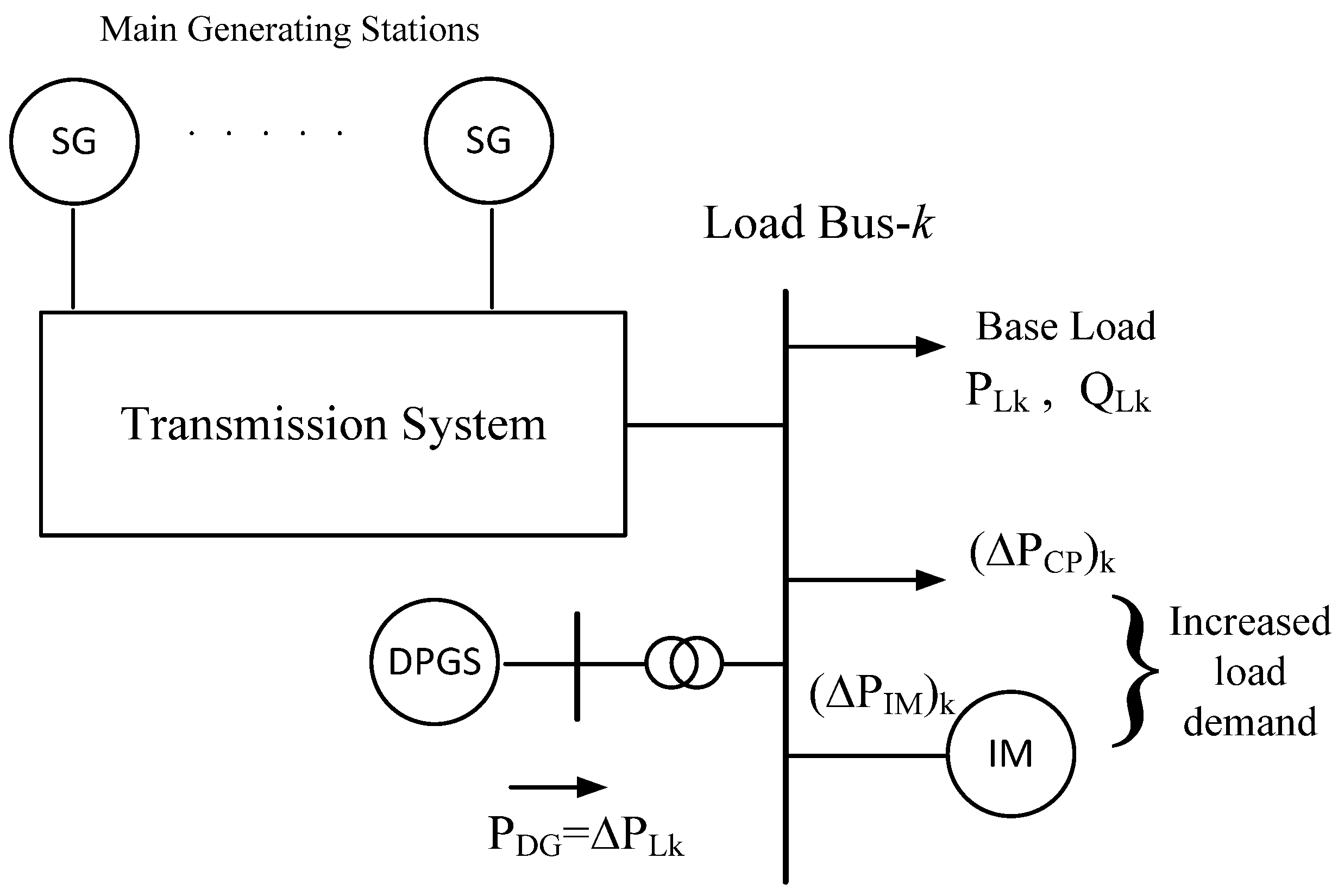
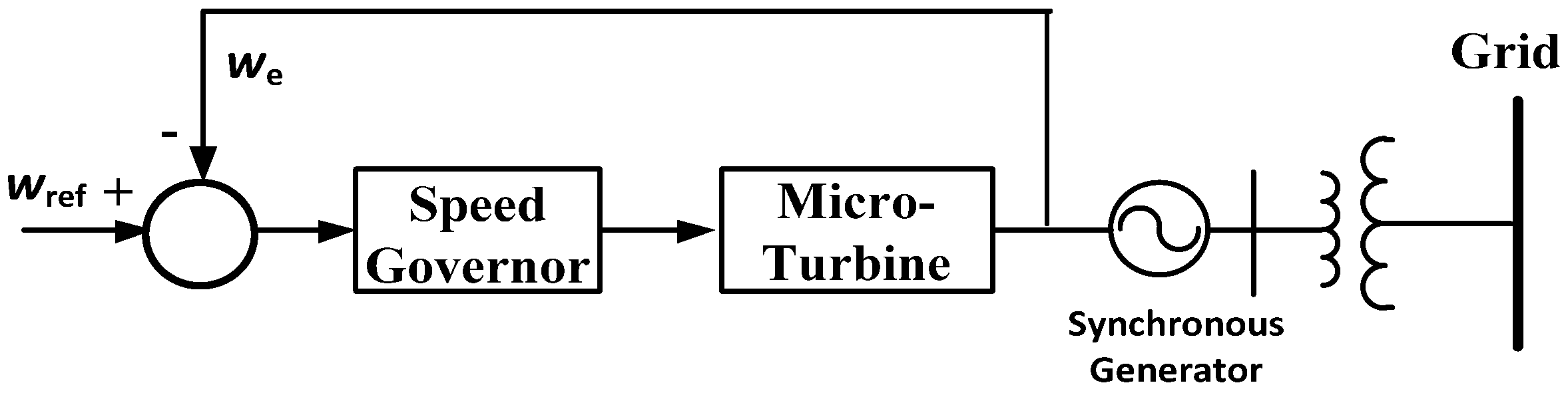
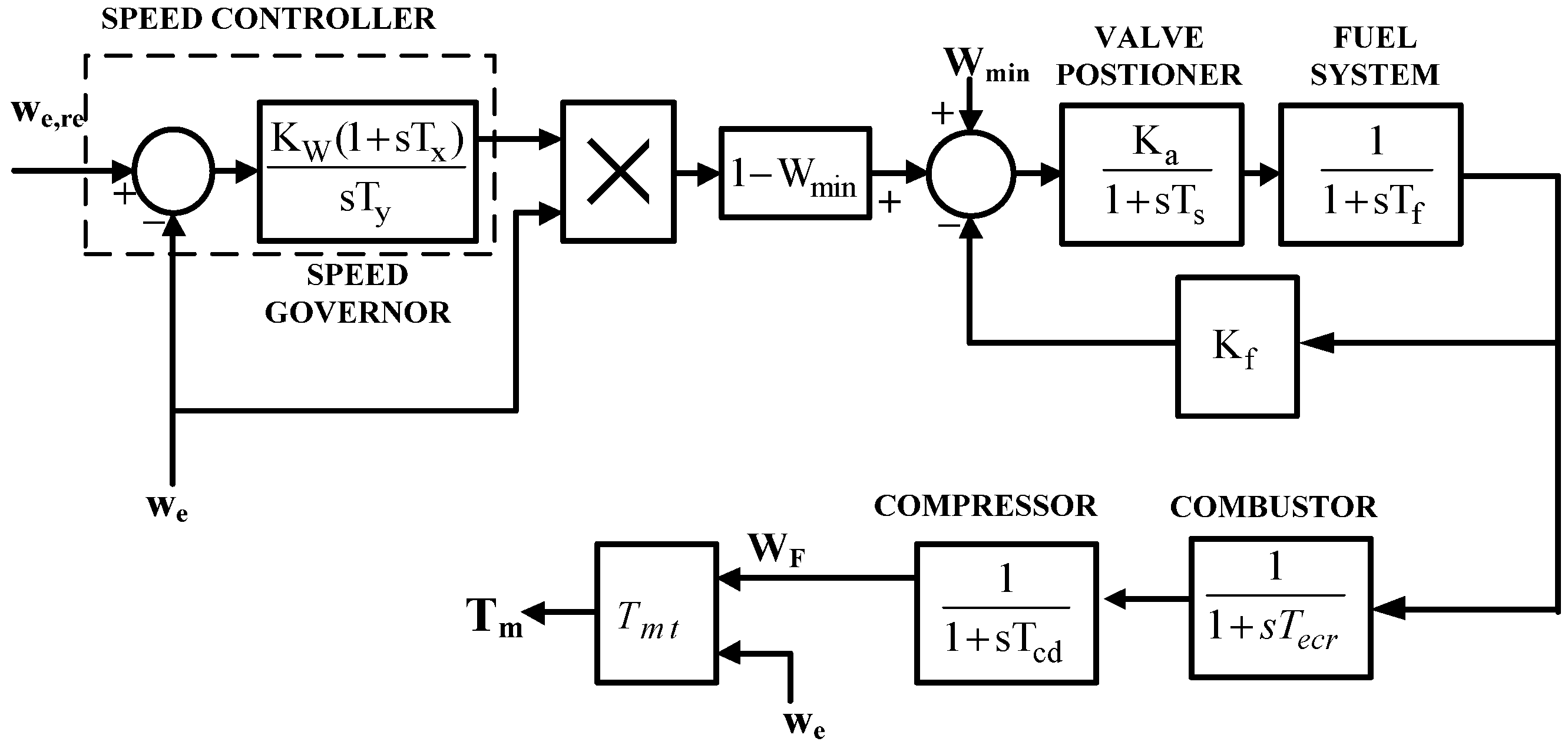
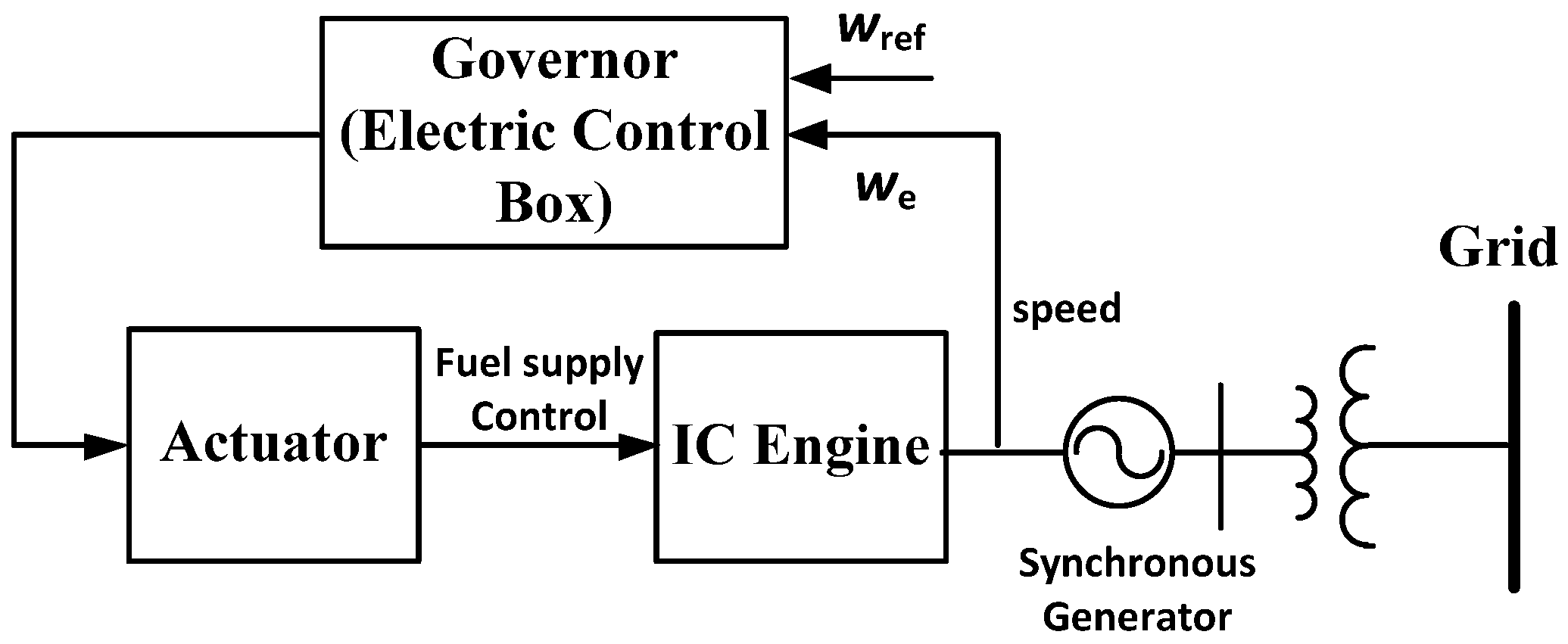
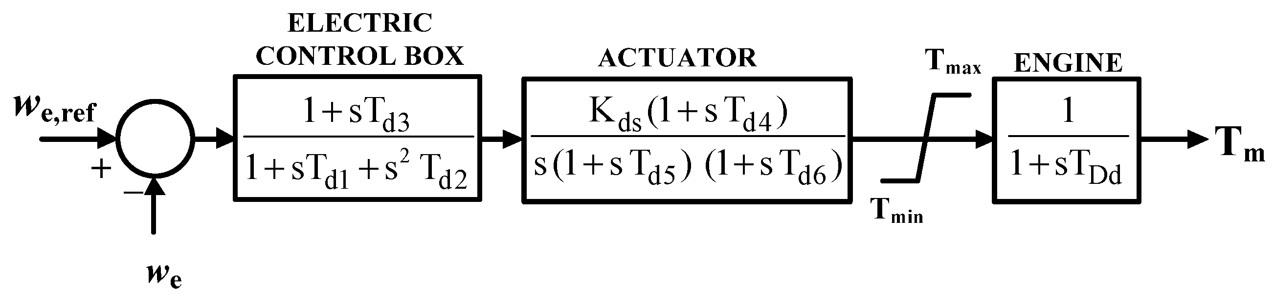
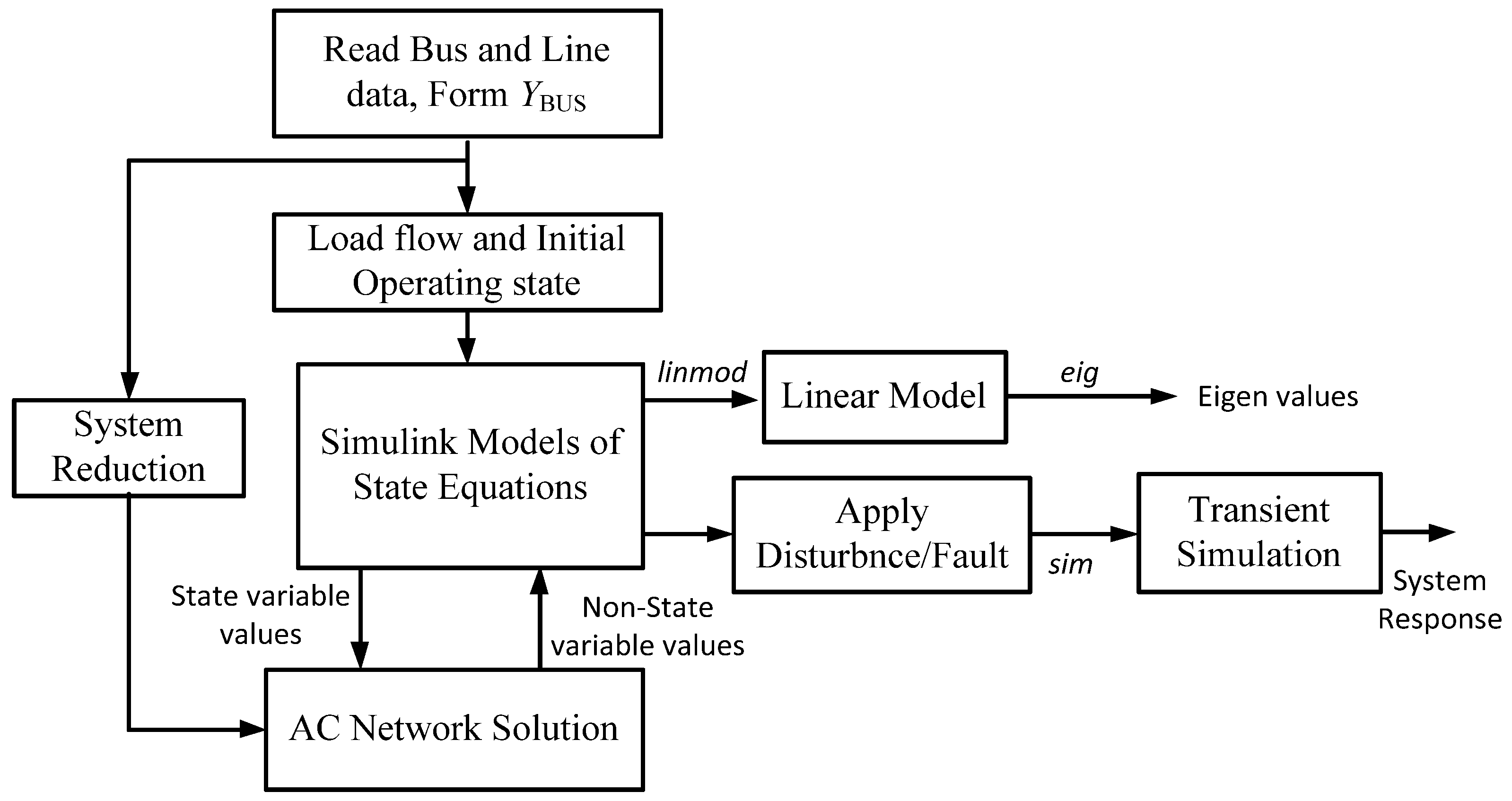

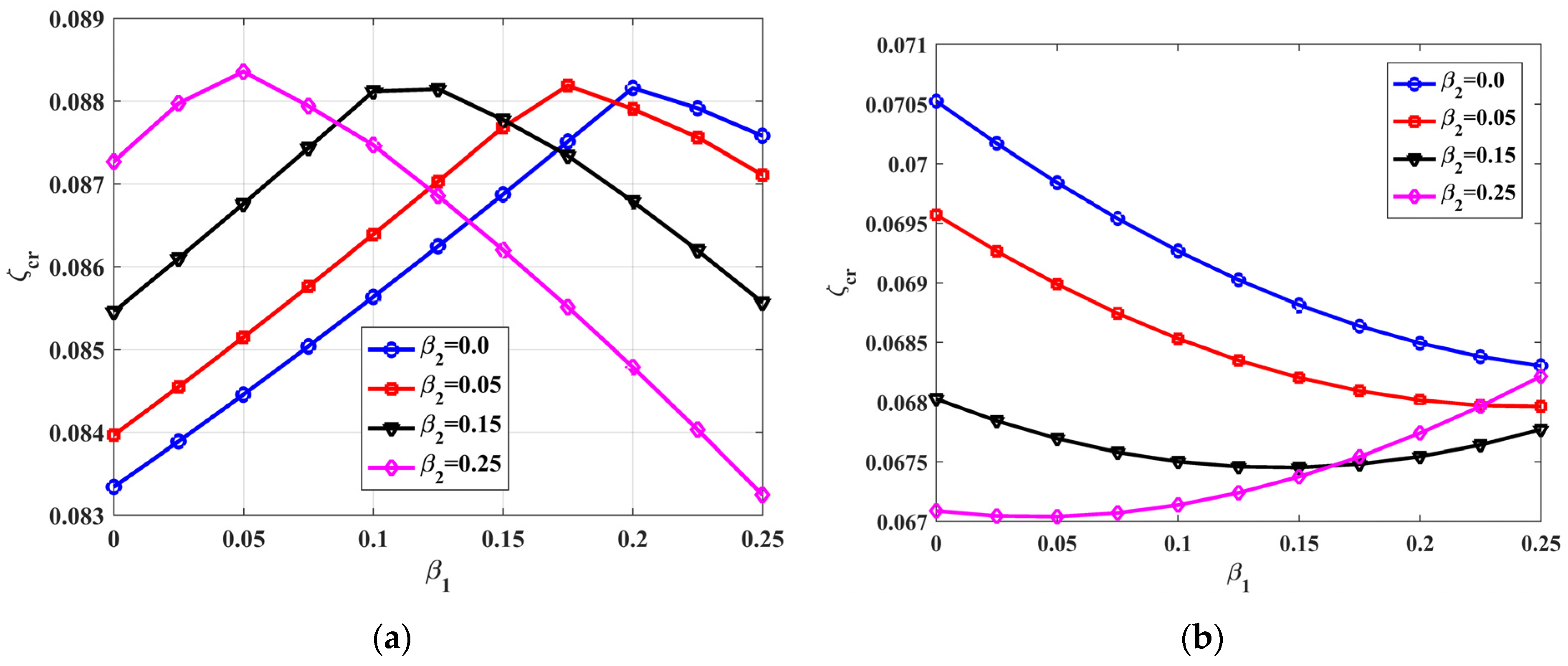

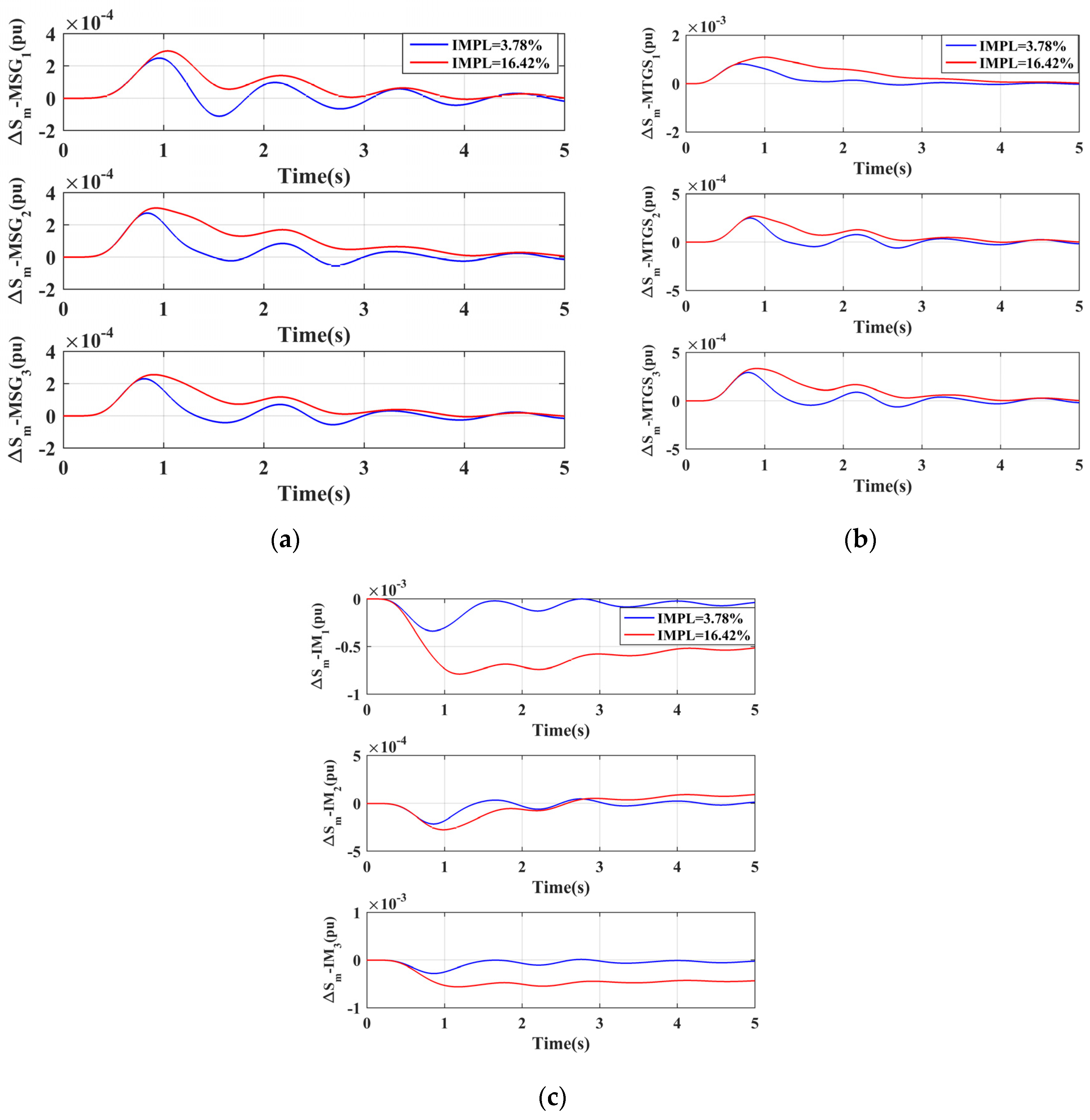
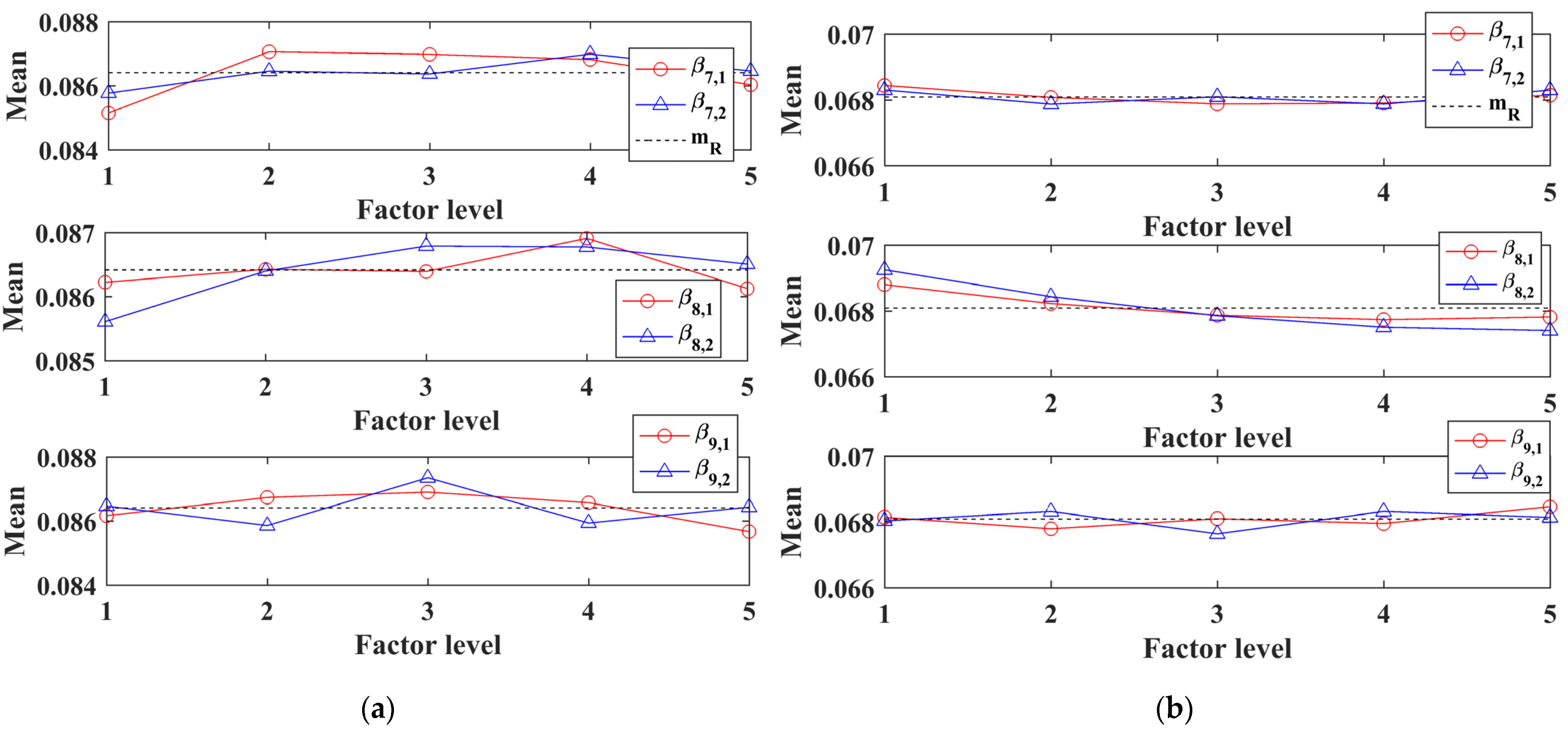
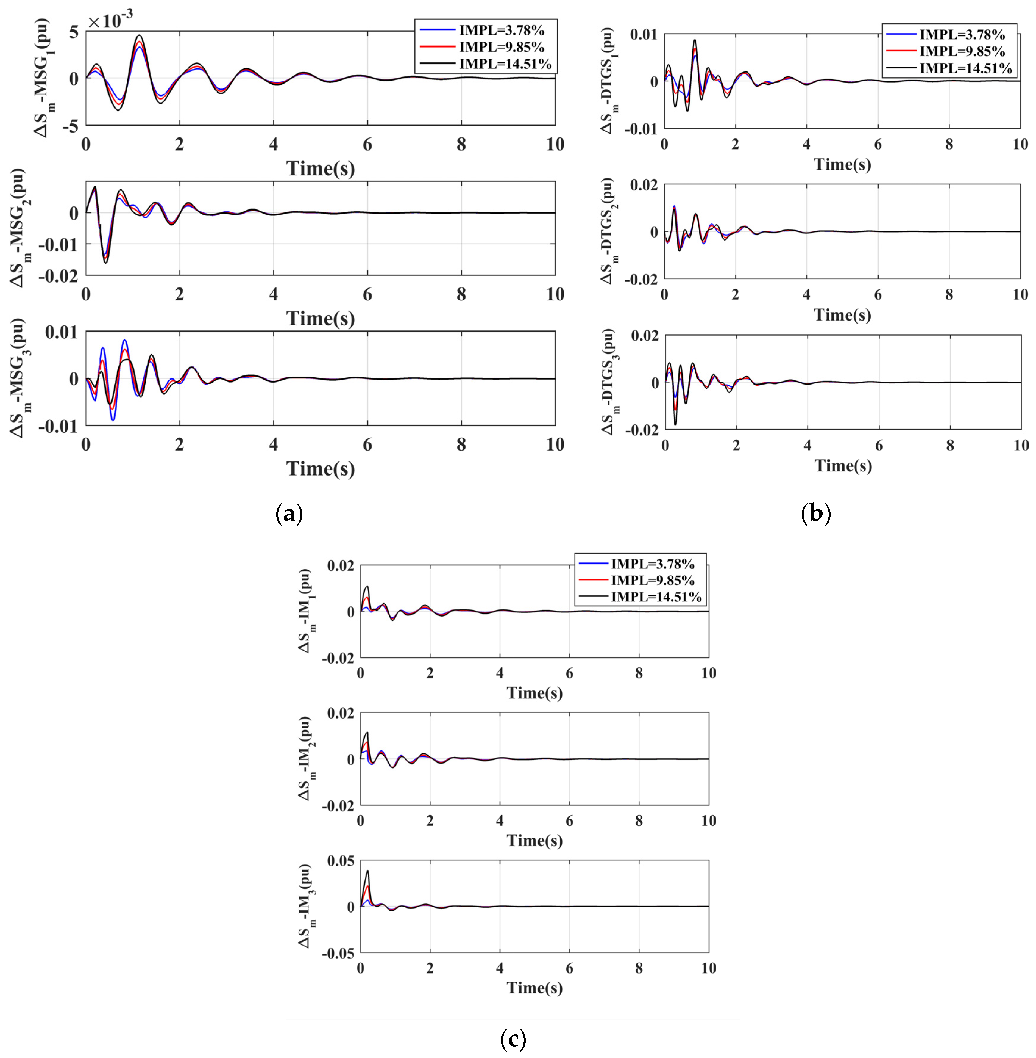
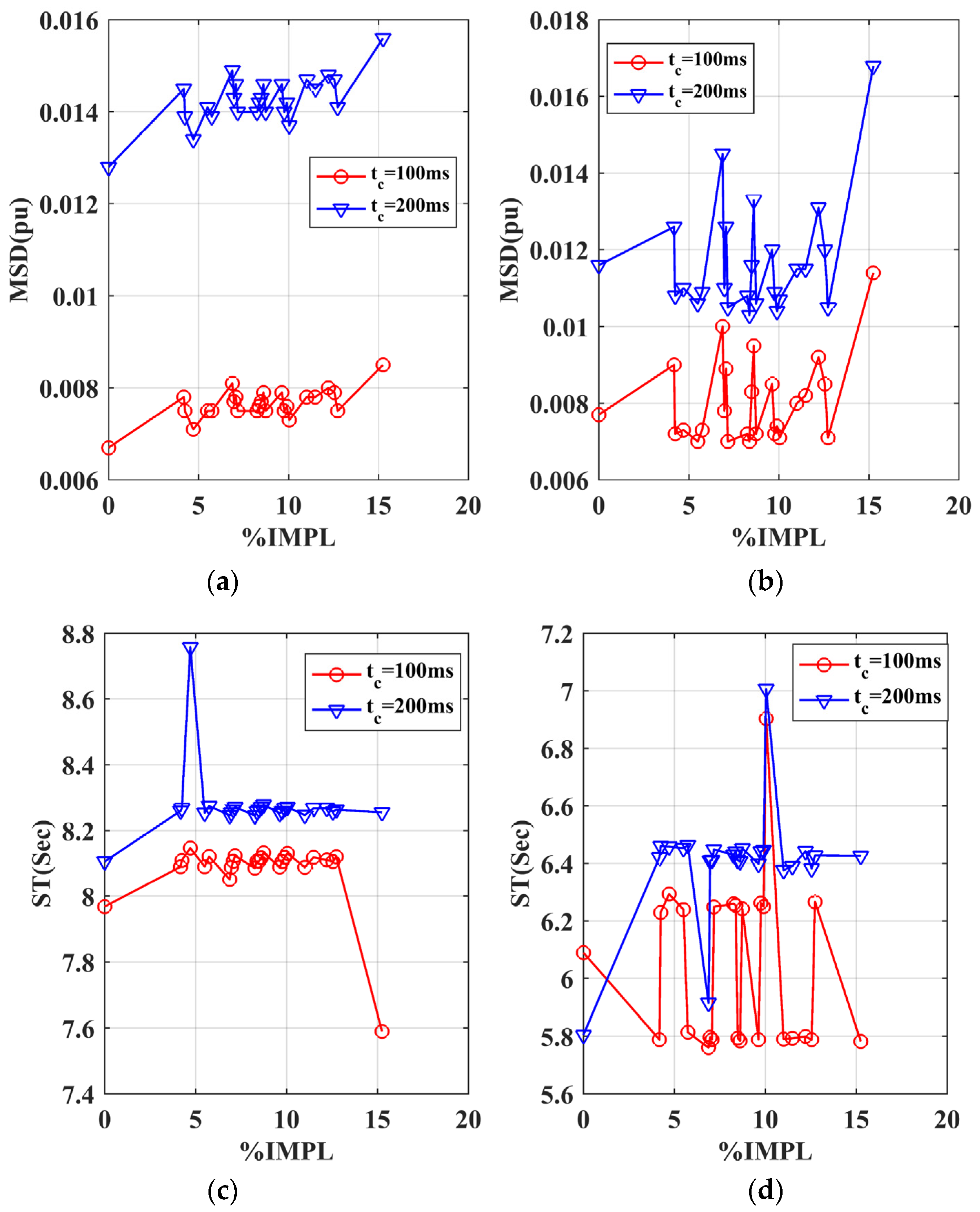
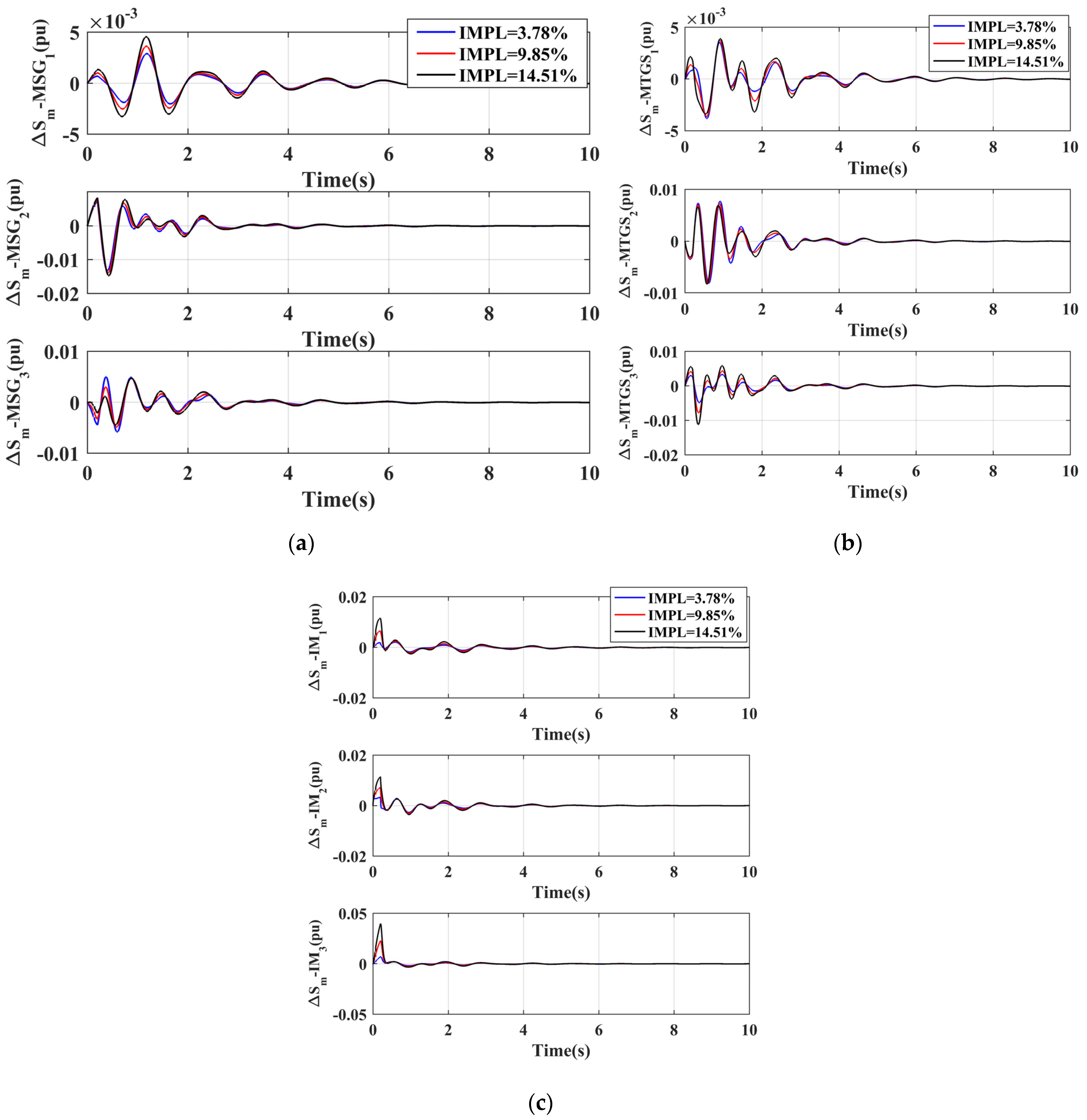
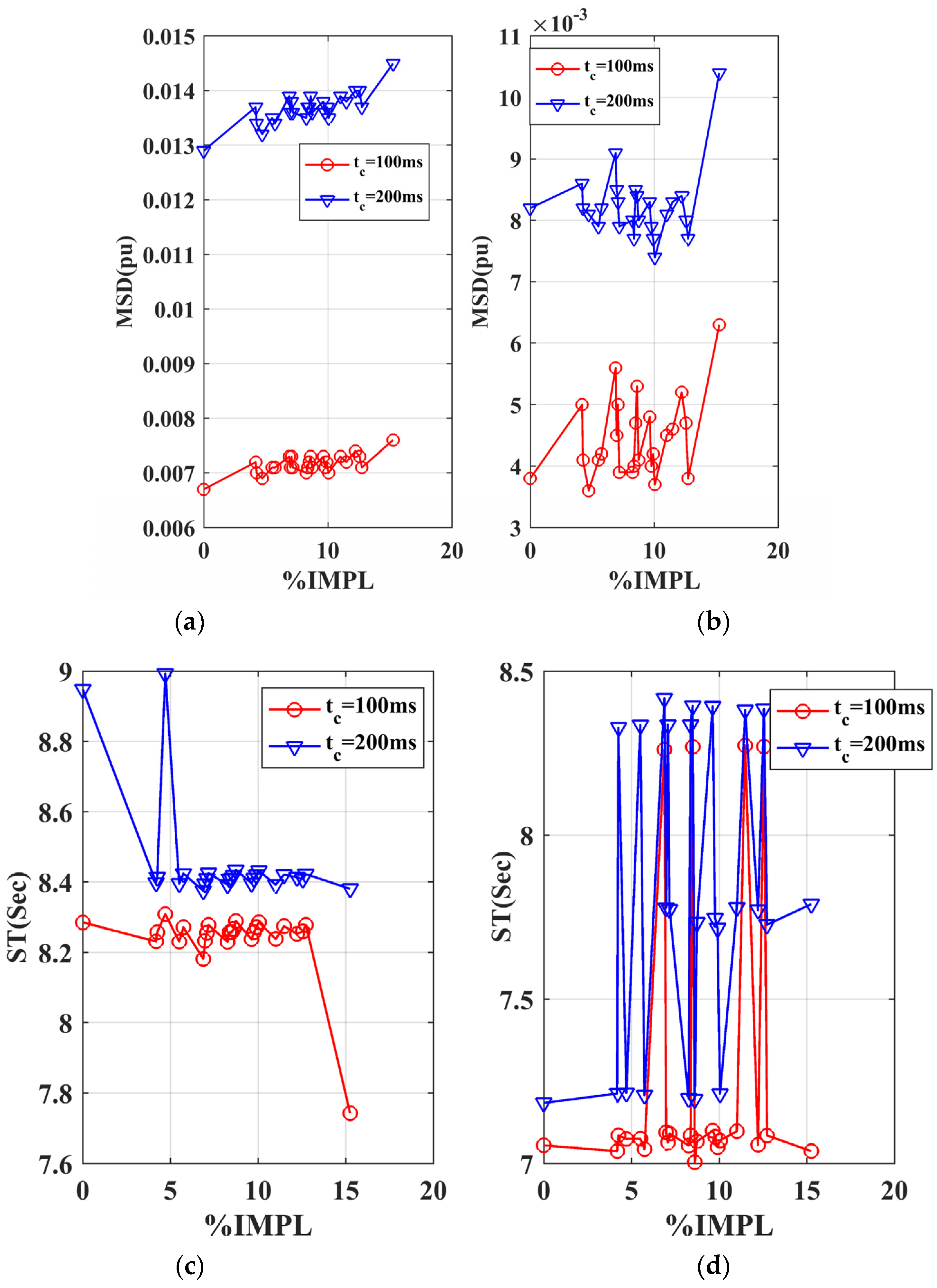
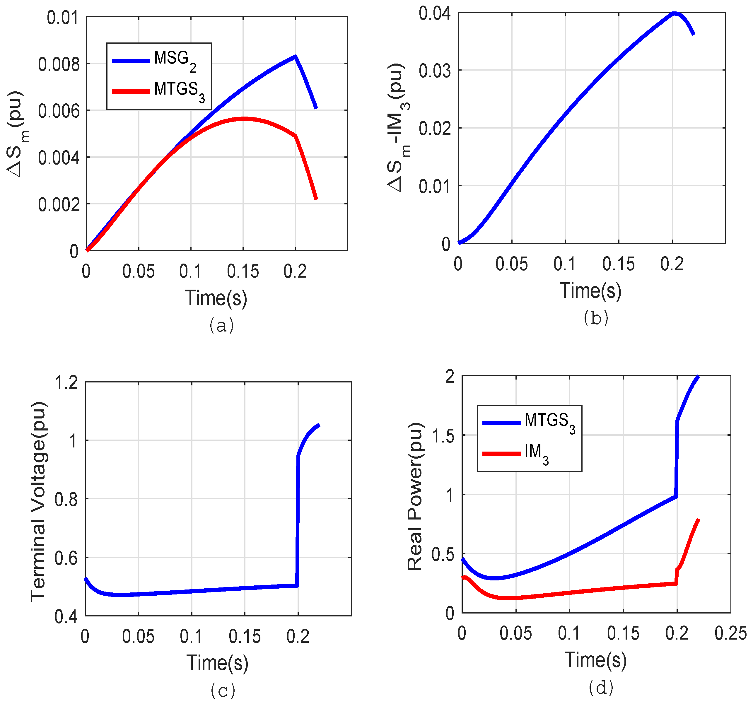
