GSA-KELM-KF: A Hybrid Model for Short-Term Traffic Flow Forecasting

Abstract

Short-term traffic flow forecasting, an essential enabler for intelligent transportation systems, is a fundamental and challenging task for dramatically changing traffic flow over time. In this paper, we present a gravitational search optimized kernel extreme learning machine, named GSA-KELM, to avoid manually traversing all possible parameters to improve the potential performance. Furthermore, with the interference of heavy-tailed impulse noise, the performance of KELM may be seriously deteriorated. Based on the Kalman filter that cleverly combines observed data and estimated data to perform the closed-loop management of errors and limit the errors within a certain range, we propose a combined model, termed GSA-KELM-KF. The experimental results of two real-world datasets demonstrate that GSA-KELM-KF outperforms the state-of-the-art parametric and non-parametric models.

1. Introduction

Accurate traffic flow forecasting is essential for many intelligent transportation systems. It not only participates in dynamic traffic management (DTM) but also provides routing information for the public traffic plans [1]. Therefore, it has attracted close attention from public institutions, commercial organizations, and individual travellers. Despite all that, short-term traffic flow forecasting is challenging because of the uncertainty of the seasonality that emerged from noise and the randomness of exogenous elements [2].

Short-term traffic flow is traffic flow with a sampling interval not exceeding 15 min. Parametric Regression (PR) and Non-Parametric Regression (NPR) are two kinds of short-term traffic flow forecasting methods [3]. PR includes moving average [4], spectral analysis [5,6], time series method [7,8], combined forecasting method [9], and Kalman filtering [10]. Parametric models with finite parameters presume that traffic flow is subordinated to a certain distribution, e.g., Gaussian distribution. It is difficult to capture the complex nonlinear relationship of traffic flow for this kind of model with the functions of finite parameters, which are prone to insufficient fitting. Non-parametric models for short-term traffic flow forecasting contain fuzzy logic systems [11], support vector regression [12], artificial neural networks [13], extreme learning machines [14,15], long short-term memory [16,17], etc.

In recent years, more and more researchers have demonstrated their interest in short-term traffic flow forecasting. A simple yet efficient learning method for complex nonlinear structures has been established based on a neural network that occupies incalculable superiority for strong learning capacity. The most popular neural networks—single-hidden layer feed-forward neural networks—have been widely utilized for traffic flow forecasting. Nevertheless, they still has the drawbacks of a slower learning speed than required, easily converging to a local minimum and over-fitting.

Extreme Learning Machine (ELM) is an improved single-hidden layer feedforward neural network learning algorithm. In ELM, the input weights and the biases are randomly generated, which is useful for overcoming the shortcomings of the above forecasting models [18]. ELM has the advantages of strong adaptability to nonlinear systems and fast speed. Wang et al. [19] proposed an ELM based on fuzzy C-means (FCM). Chen et al. [20] apply the maximum mixture correntropy criterion (MMCC) to ELM for function approximation and data regression. For all that, the method needs to set the number of hidden layer neurons. To further enhance the performance of ELM and satisfy some particular application requirements, the implicit mappings defined by the kernel could be employed to replace the explicit feature mappings. Along this line of thought, KELM provides a junction point for ELM with several classical learning methods, e.g., the radial basis function network [21] and the least squares support vector machine [22].

It is noteworthy that KELM finds the optimal parameters suitable for the model via the grid search method, which causes a small learning rate, an overly long learning time, over-fitting, degradation of generalization performance, etc. Furthermore, the minimum mean square error is dependent on the assumption that the data are noise-free or the noise is of Gaussian distribution. The performance may deteriorate seriously when some heavy-tailed impulsive noises disturb the distribution of data in KELM.

Many algorithms have been reformulated to address these issues, such as the genetic algorithm and gravitational search algorithm [23,24,25,26]. In this paper, the kernel extreme learning machine optimized by GSA is proposed, which does not need to manually traverse all possible parameter combinations of $\gamma$ and $\sigma$ to achieve more accurate forecasting performance. And, the GSA-KELM combined Kalman filter model effectively reduces the interference of heavy-tailed impulse noise.

The major contributions of this work are shown as follows.

• First, we retain the advantages of KELM’s implicit mapping and optimize the KELM through the GSA to avoid manually traversing all possible parameters and improve potential accuracy.
• Second, the GSA-KELM combined Kalman filter model effectively reduces the interference of heavy-tailed impulse noise.
• Third, the outperformance of our model is demonstrated on two benchmark datasets via comparison with several benchmark methods for traffic flow forecasting.

The rest of this paper is organized as follows. The second part is the methodology, the third part is the experiment, and the fourth part is the conclusion.

2. Methodology

This section briefly introduces the gravitational search algorithm, kernel extreme learning machine, and Kalman filter as shown in Figure 1. Then, we employ GSA-KELM and KF to forecast traffic flow. Lastly, we detail the combination of GSA-KELM and KF.

2.1. Gravitational Search Algorithm

The gravitational search algorithm (GSA) [27] is a heuristic search algorithm inspired by Newtonian laws of gravity. Its main idea is that any two particles attract each other through the force connecting the centre line direction.

Assuming k particles in d-dimensional search space, the position of the i-th particle can be expressed as ${\mathit{X}}_i=(x_i^1,x_i^2,\dots ,x_i^d)$ for $\mathit{i}=1,2,\dots ,k$. And the velocity can be expressed as ${\mathit{V}}_i=(v_i^1,v_i^2,\dots ,v_i^d)$. The inertial mass of particles can be updated by

$$\begin{array}{cc}\hfill {fit}_i& \left(t\right)={fv}_i\left(t\right)-{fv}_i(t-1),\hfill \\ \hfill m_i\left(t\right)& =\frac{\left|{fit}_i\left(t\right)\right|-max|{fit}_i\left(t\right)|}{min|{fit}_i\left(t\right)|-max|{fit}_i\left(t\right)|},\hfill \\ \hfill & M_i\left(t\right)=\frac{m_i\left(t\right)}{{\sum }_{j=1}^k{m}_j\left(t\right)},\hfill \end{array}$$

(1)

where $f{v}_i\left(t\right)$ is the fitness value of the i-th particle at iteration t. And the initial value is set to 0. The gravitation force exerted by the j-th particle to i-th particle at tth iteration is defined by

$$F_{ij}^d\left(t\right)=G\left(t\right)\frac{M_j\left(t\right)\times M_i\left(t\right)}{D_{ij}\left(t\right)+r}(x_j^d\left(t\right)-x_i^d\left(t\right)),$$

(2)

where $M_j\left(t\right)$ and $M_i\left(t\right)$ are the inertial masses of the particle j, which exerts the gravity and the acted particle i, respectively; $D_{ij}\left(t\right)$ denotes the Euclidian distance between i-th particle and j-th particle; and r is a small constant. $G\left(t\right)$ is a gravity constant that controls the search accuracy, indicated by

$$G\left(t\right)=G_0{e}^{-v\frac{t}{T}},$$

(3)

where $G_0$ denotes the initial value of the gravity constant, v is the manually adjusted constant, and T is the utmost iteration. Similarly, the  acceleration is expressed by

$$a_i^d\left(t\right)=\frac{F_i^d\left(t\right)\times {fit}_i\left(t\right)}{M_i\left(t\right)\times \left|{fit}_i\left(t\right)\right|},$$

(4)

In each iteration, the particle updates its position and speed, which can be represented as

$$\begin{array}{c}\hfill v_i^d(t+1)=rando{m}_i\times v_i^d\left(t\right)+a_i^d,\\ \hfill x_i^d(t+1)=x_i^d+v_i^d(t+1).\end{array}$$

(5)

Obviously, given the initial value of particle position and velocity, the optimal position of the particle is obtained after a series of update calculations and after the optimal fitness value is figured out.

2.2. Kernel Extreme Learning Machine

The Extreme Learning Machine (ELM) is a single hidden layer feed-forward neural network, whose general form with L hidden layer neurons is described in Equation (6).

$$f_L\left(X\right)={\displaystyle \sum _{i=1}^L}{\beta }_i{g}_i\left(X\right)={\displaystyle \sum _{i=1}^L}{\beta }_{i}g(a_i,b_i,X),$$

(6)

where ${\beta }_1,{\beta }_2,\dots ,{\beta }_L$ are the output weights between the hidden layer with L neurons and the output layer, and $g_i$ is activation function, whose parameters $a_i$ and $b_i$ are randomly assigned [28]. The output weight of the ELM is directly computed by minimizing the approximation error described in Equation (7).

$$\underset{\beta ϵR_{L\times N}}{min}{\parallel H\beta -Y\parallel }^2,$$

(7)

where H is the output of the hidden layer with L neurons, N is the number of neurons in the output layer, and Y is the target matrix of training data. The solution to Equation (8) is

$$\beta ={(\gamma \mathbf{I}+H^{T}H)}^{-1}{H}^{T}Y),$$

(8)

where $\mathbf{I}$ is an identity matrix. For a new input $\mathbf{x}$, the output can be expressed as

$$f\left(x\right)=h\left(\mathbf{x}\right)\beta .$$

(9)

After introducing the kernel function [29,30], the explicit feature mappings can be replaced by implicit mappings, which means that $h\left(\mathbf{x}\right)$ does not need to be known. In this paper, the Gaussian kernel [31], the most popular kernel, is chosen. The expression is

$$\kappa ({\mathbf{x}}_1,{\mathbf{x}}_2)=exp(-\frac{\parallel {\mathbf{x}}_1-{\mathbf{x}}_2\parallel }{2{\sigma }^2}),$$

(10)

where $\sigma$ is the kernel size. Therefore, the trouble of manually adjusting the number of hidden nodes and randomly generating the input weights and biases is omitted [32]. Then, the expression is converted to

$$\begin{array}{cc}\hfill f\left(\mathbf{x}\right)& =\phi \left(\mathbf{x}\right)\beta \hfill \\ \hfill & =\phi \left(\mathbf{x}\right){(\gamma \mathbf{I}+{\varphi }^T\varphi )}^{-1}{\varphi }^{T}Y\hfill \\ \hfill & =\phi \left(\mathbf{x}\right){\varphi }^T{(\gamma \mathbf{I}+{\varphi }^T\varphi )}^{-1}Y\hfill \\ \hfill & =\mathbf{k}\left(\mathbf{x}\right)\alpha ,\hfill \end{array}$$

(11)

where $\alpha ={(\gamma \mathbf{I}+{\varphi }^T\varphi )}^{-1}Y$ is the coefficient matrix and $\mathbf{k}\left(\mathbf{x}\right)=\phi \left(\mathbf{x}\right){\varphi }^T$. The kernel trick [33] can be described by $\phi \left({\mathbf{x}}_1\right)\phi {\left({\mathbf{x}}_2\right)}^T$=$\kappa ({\mathbf{x}}_1,{\mathbf{x}}_2)$. Therefore, having

$$\begin{array}{cc}\hfill \phi \left(\mathbf{x}\right){\varphi }^T& =\phi \left(\mathbf{x}\right)[\phi {\left({\mathbf{x}}_1\right)}^T,\dots ,\phi {\left({\mathbf{x}}_N\right)}^T]\hfill \\ \hfill & =[\kappa (\mathbf{x},{\mathbf{x}}_1),\dots ,\kappa (\mathbf{x},{\mathbf{x}}_N)],\hfill \end{array}$$

(12)

and

$$\varphi {\varphi }^T=\left[\begin{array}{cccc}& \kappa ({\mathbf{x}}_1,{\mathbf{x}}_1)& \cdots & \kappa ({\mathbf{x}}_1,{\mathbf{x}}_N)\\ & ⋮& \ddots & ⋮\\ & \kappa ({\mathbf{x}}_N,{\mathbf{x}}_1)& \cdots & \kappa ({\mathbf{x}}_N,{\mathbf{x}}_N)\end{array}\right]$$

(13)

2.3. Kalman Filter

The Kalman filter (KF) [34], a kind of prediction method based on the filtering principle proposed by Kalman in 1960, is suitable for estimating the optimal state of a dynamic system. Before being applied to short-term traffic flow prediction, it has been successfully applied in traffic demand prediction with high prediction accuracy.

The basic principle of the Kalman filter is to establish the state space model of the sampled signal, and its mathematical model is expressed as

$${\mathbf{x}}_{t+1}=F{\mathbf{x}}_t+{\omega }_t,$$

(14)

$${\mathbf{y}}_{(t+1)}=H{\mathbf{x}}_t+{\nu }_t.$$

(15)

Equation (14) is the state of the system, and Equation (15) is the system observation. F is state transfer matrix, and H is the observation matrix. ${\omega }_t$ is random variables for the process noise, and ${\nu }_t$ is the observation noise, both of which obey independent Gaussian distribution.

$$\begin{array}{cc}\hfill p\left(\omega \right)& \sim \mathit{N}(0,Q),\hfill \\ \hfill p\left(\nu \right)& \sim \mathit{N}(0,R)\hfill \end{array}$$

(16)

where Q and R are processed error covariance and observation error covariance.

The Kalman filter estimates the prior state ${\widehat{x}}_t^{-}$ and $P_t^{-}$ by recursively updating the a posteriori estimation ${\widehat{x}}_t^{+}$ of the state and the covariance of the estimation error $P_t^{+}$ by the following equations:

$${\widehat{x}}_t^{-}=F{\widehat{x}}_{t-1}^{+},$$

(17)

$$P_t^{-}=F{P}_{t-1}^{+}{F}^T+Q,$$

(18)

$$K_t=P_t^{-}{H}_t^T{(H_t{P}_t^{-}{H}_t^T+R)}^{-1},$$

(19)

$${\widehat{x}}_t^{+}={\widehat{x}}_t^{-}+K_t(x_t-H_t{\widehat{x}}_t^{-}),$$

(20)

$$P_t^{+}=(I-K_t{H}_t)P_t^{-},$$

(21)

where $K_t$ is the Kalman filter gain, I is the identity matrix, and $x_t$ is Observation.

2.4. GSA-KELM for Traffic Flow Forecasting

It is a tremendous project in KELM using the grid search method to manually operate potential values of $\gamma$ and $\sigma$. However, massive parameter values are vital to achieving the expected performance.

To settle the aforementioned problems, the gravitational search algorithm takes the place of the grid search method to search for more suitable network parameters for the KELM, termed GSA-KELM. First, the particles are initialized by setting the spatial dimensions, number of particles, gravity constant, gravitational force constant, value of fit, and maximum iteration number. Then, the positions and velocities of particles are generated randomly, and the initial fit value is zero. After that, the fitness value of particles is calculated in KELM. Later, the positions and velocities of particles are updated for optimum fitness until the ultimate criteria are met. The algorithm of GSA-KELM is shown in Algorithm 1.

Algorithm 1: Framework of GSA-KELM

Input: Training set S = ${\{x_j,y_j\}}_{j=1}^N$

Output: The value of fitness

1 Parameters setting: spatial dimensions d, the number of particles k in a d-dimensional search space, gravity constant G, constant r for the gravitational force, and maximum iteration number T.

2 Initialization: Positions x and velocities v of randomly generated Q groups of particles.

3 for t = 1 to T do

2.5. Kalman Filter for Traffic Flow Forecasting

Kalman filter is a good predictor for the near future with a basic implementation process as follows. First, the forecast period data are input, and the model is initialized. Then, the prior estimate ${\widehat{x}}_t^{-}$ and prior covariance of the estimation error $P_t^{-}$ are calculated by Equation (17) and Equation (18), respectively. In Equation (19), the Kalman filter gains $K_t$ are calculated. Later, the posterior estimate ${\widehat{x}}_t^{+}$ is acquired by Equation (20), and the posterior covariance $P_t^{+}$ is obtained by Equation (21) to predict the next time. The algorithm is shown in Algorithm 2.

Algorithm 2: Framework of KF.

Input: $F,H,Q,R,P_{T_0}^{+},{\widehat{x}}_{t_0}^{+}$

Output: ${\widehat{x}}_{t+1}$, t = $T_0,\dots ,T_c$

1 for t = $T_0$ to $T_c$ do

2.6. GSA-KELM-KF Model for Traffic Flow Forecasting

In reality, most data are collected by instruments. Heavy-tailed impulsive noises are unavoidable, disturbing data distribution in GSA-KELM. The reason the Kalman filter is widely used in traffic flow prediction is not that its estimation deviation is small. The observation data and estimation data are skillfully combined in the KF, which conducts closed-loop management of error and limits the error to a certain range. Thus, combining the Kalman filter with GSA-KELM can effectively reduce the influence of heavy-tailed pulse noise. In this paper, the linear combination method is adopted, and it can be expressed as

$$\widehat{y}=\eta {\widehat{y}}_{gk}+(1-\eta ){\widehat{y}}_{kf},$$

(22)

where ${\widehat{y}}_{gk}$ and ${\widehat{y}}_{kf}$ are the prediction results of GSA-KELM and KF, respectively. $\eta$ is the weight, and the value range is $(0,1)$.

The prediction process can be described as follows. Firstly, calculate the forecast results of GSA-KELM and KF. Then, select the weight value. Finally, obtain the forecast results of the GSA-KELM-KF through Equation (22). The algorithm is shown in Algorithm 3. The flow chart is shown in Figure 1.

Algorithm 3: Framework of GSA-KELM-KF

Input: Training set S = ${\{x_j,y_j\}}_{j=1}^N$

Output: The forecast results of the Emsemble

1 Initialize parameters.

2 Use GSA-KELM and KF to predict the traffic flow of the selected period, and the results are stored as ${\widehat{y}}_{gk}$ and ${\widehat{y}}_{kf}$, respectively.

3 The results $\widehat{y}$ are obtained by Equation (22).

3. Experiments

In this section, the performance of the GSA-KELM-KF model is evaluated on two publicly benchmark datasets for short-term traffic flow forecasting, e.g., the Amsterdam high-way dataset and England M25 highway dataset. More specific details are given below.

3.1. Datasets Description

The Amsterdam highway dataset was collected on four motorways, namely, A1, A2, A4, and A8, in Amsterdam, the Netherlands. The basic conditions of the four expressways are shown in Figure 2. The four benchmark datasets, each of which consists of five weeks of data collected by the MONICA annular detector from 20 May to 24 June 2010, are aggregated by vehicles per minute and hour. Traffic flow data of 1 min are aggregated into 10-min aggregation in the same method. In the raw data, erroneous data are mixed, e.g., zero or negative for a long time. The average of the measurements at the same time in other weeks is used to revise them.

England M25 highway dataset was collected from seven stations, namely, D1, D2, D3, D4, D5, D6, and P in England. Each station contains four weeks of data, collected per 15 min from 1 August 2019 to 31 August 2019. The measurement positions are near Heathrow Airport on the M25 expressway, as shown in Figure 3.

3.2. Evaluation Criteria

In this paper, some frequently used criteria are employed to evaluate the performance of the GSA-KELM-KF model. The root means square error (RMSE) measures the average differences between the predictions of a model and the system being modelled, while the mean absolute percentage error (MAPE) is the percentage expression of the differences. Their expression is as follows:

$$RMSE=\sqrt{\frac{1}{N}{\displaystyle \sum _{k=1}^N}{(\widehat{y}\left(k\right)-y\left(k\right))}^2},$$

(23)

$$MAPE=\frac{1}{N}{\displaystyle \sum _{k=1}^N}\left|\frac{\widehat{y}\left(k\right)-y\left(k\right)}{y\left(k\right)}\right|\times 100\%,$$

(24)

where $y\left(k\right)$ is the groundtruth, and $\widehat{y}\left(k\right)$ is the prediction at the time k.

3.3. Experimental Setup

All experiments are compiled and tested on a Linux cluster (CPU: Intel(R) Xeon(R) Platinum 8255C CPU @ 2.50GHz, GPU: NVIDIA GeForce RTX 3070).

For KF, this paper adopts the prediction strategy of predicting the current time from the previous time, so H is set to $\left[1\right]$. F is the identity matrix. And the initialization covariance matrix is consistent with Q.

Amsterdam highway dataset is divided into two parts: the first four weeks for training and the last week for testing. Each input vector contains 12 consecutive data values to forecast the value of the 13th data value. The ranges of the positions and velocities of $\gamma$ are set to $[{10}^{-3},{10}^{-1}]$ and $[-{10}^{-4},{10}^{-1}]$, while the ranges of positions and velocities of $\theta$ are $[0.1,15]$ and $[-2,2]$. In KF, the R is set as $0.2$. Q of dataset A1 is set $4\times {10}^{-2}I$, and the other settings are ${10}^{-2}I$. The value of $\eta$ of dataset A1 and dataset A2 is $0.9$, and the others are $0.7$.

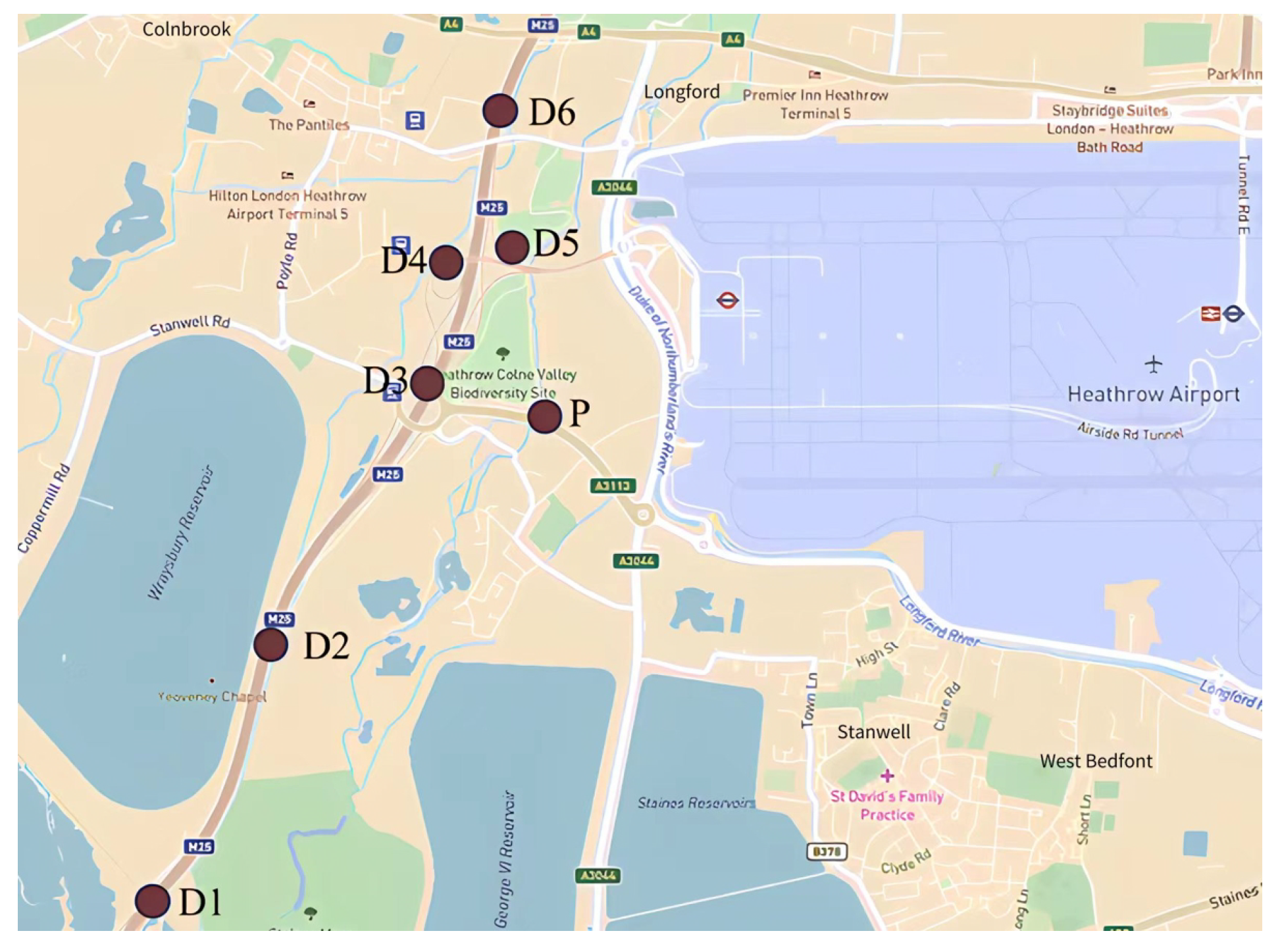
England M25 highway dataset is also split into two parts: the first week for training and the second week for testing. The dimensions of the network are set to 12. In the gravity search algorithm, the maximum number of iterations is set to 50. The ranges of the positions and velcocities of $\gamma$ are set to $[{10}^{-3},{10}^{-1}]$ and $[{-10}^{-4},{10}^{-1}]$. $[0.5,30]$ and $[-5,5]$ are the ranges of the positions and velocities of $\theta$. In KF, R and $\eta$ are set to $0.1$ and $0.9$. Q of datasets D4 and P is set ${10}^{-3}I$ and ${10}^{-4}I$, respectively, while the other settings are ${10}^{-2}I$.

To evaluate the performance of the GSA-KELM-KF framework, we compared it with the support vector machine regression, decision tree, artificial neural network, k-nearest neighbour, long short-term memory, noise-immune long short-term memory, extreme learning machine, and kernel extreme learning machine frameworks.

Support vector machine regression (SVR): SVR adds the tolerance deviation of ∈ between the estimated value and the real value to minimize the total deviation of all sample points from the hyperplane. The radial basis function is used as the kernel type, whose regression horizon and the width parameter are set to 8 and $3\times {10}^{-6}$. The cost parameter is set to the maximum difference for short-term traffic flow forecasting.

Decision tree (DT): Based on classification and regression tree, DT has strong robustness for missing data and noise without any prior hypothesis [35].

Artificial neural network (ANN): ANN, a learning model, is generated by the interconnection of a large number of neurons. The number of hidden layers, the mean squared error goal, the spread of radial basis functions, the maximum number of neurons in the hidden layer, and the number of neurons to add between displays based on a default values are set to 1, $0.001$, 2000, 40, and 25, respectively [36].

k-nearest neighbor (kNN) [37]: kNN is a machine learning algorithm with a high tolerance for outliers and noise. Predict the properties of a query vector by using the properties of the few vectors closest to the query vector.

Long short-term memory (LSTM) [38]: LSTM is a special kind of recurrent neural network. It is developed to capture time dependence over a long period for traffic flow forecasting. Optimized by grid search, the validation split, the epochs, the batch size, and the hyperparameter units are $0.05$, 50, 32, and 256, respectively.

Noise-immune long short-term memory (NiLSTM) [39]: A noise immunity loss function is derived through the maximum correlation entropy of long short-term memory networks. Compared with conventional LSTM, the loss of maximum correlation entropy is a local similarity measure and is not immune to non-Gaussian noise. The length of the input sequence is set to 12, and the range of kernel size is $[0.1,0.2,0.5,1.0,2.0,3.0]$.

Extreme learning machine (ELM) [40]: ELM is a single-hidden layer feed-forward neural network, which can be directly applied to regression, classification, clustering, and other learning tasks. Both the input weights and the biases of the hidden layer are generated randomly.

Kelnel extreme learning machine (KELM): KELM, as a variety of extended ${ELM}_s$, improves the generalization of ELM, in which the explicit feature mappings are replaced by kernels according to the kernel method. It is unnecessary to allocate the input weights and biases [41,42]. In KELM, the parameters $\gamma$ and $\sigma$ are set to $\{{10}^{-5},{10}^{-4},{10}^{-3},{10}^{-2},{10}^{-1}\}$ and {0.01, 0.05, 0.1, 0.3, 0.5, 0.7, 1, 3, 5, 7, 10, 15, 30, 60, 120}.

3.4. Experimental Result

To verify the effectiveness of the proposed models for the randomness and nonlinearity of traffic flow, the experimental scenario in Amsterdam’s ring road dataset is introduced.

Table 1. The ${RMSE}_s$ of different forecasting models on Amsterdam high way dataset.

Models	A1	A2	A4	A8
SVR	329.09	259.74	253.66	190.30
DT	316.57	224.79	243.19	238.35
ANN	299.64	212.95	225.86	166.50
kNN	289.33	211.79	231.79	166.39
LSTM	294.52	211.31	224.68	168.91
NiLSTM	285.54	203.69	223.72	163.25
ELM	294.10	201.67	222.07	169.15
KELM	284.83	193.58	221.36	162.84
GSA-KELM-KF	283.67	192.25	216.78	162.21

Bold indicates optimal value.

and

Table 2. The ${MAPE}_s$ of different forecasting models on Amsterdam highway dataset.

Models	A1	A2	A4	A8
SVR	14.34	12.22	12.23	12.48
DT	12.08	10.86	12.34	13.62
ANN	12.61	10.89	12.49	12.53
kNN	11.57	10.42	12.19	11.70
LSTM	12.82	11.06	13.71	12.56
NiLSTM	12.00	10.14	11.57	11.76
ELM	11.82	10.34	12.05	12.42
KELM	11.76	9.75	11.37	12.79
GSA-KELM-KF	11.57	9.58	11.20	12.15

Bold indicates optimal value.

indicate the results of ${RMSE}_s$ and ${MAPE}_s$ separately.

Table 1 shows the comparison of different methods on the A1, A2, A4, and A8 datasets. Our GSA-KELM-KF outperforms typical parametric and non-parametric methods on the ${RMSE}_s$ of all datasets, whose results are $283.67$, $192.25$, $216.78$, and $162.21$, respectively. For example, compared with LSTM, the RMSE of the GSA-KELM-KF on the A1, A2, A4 and A8 datasets are decreased by $3.68\%$, $9.01\%$, $3.51\%$, and $3.96\%$, respectively. As for ELM, the RMSE of our GSA-KELM-KF are reduced by $3.54\%$, $4.67\%$, $2.38\%$, and $4.10\%$, respectively. Similarly, the RMSE of our GSA-KELM-KF are lower than KELM $0.41\%$, $0.68\%$, $2.07\%$, and $0.38\%$, respectively.

Although RMSE is more suitable for showing larger deviations, MAPE has the simplest interpretation and can be used to compare accuracy between different volumes studied [43]. Furthermore, MAPE is more suitable for the comparison of long-time series. From Table 2, we know that our GSA-KELM-KF achieves the best performance on MAPE except for the A8 dataset, with results of $11.57$, $9.58$, $11.20$, and $12.15$, respectively. Compared with LSTM, the MAPE of the GSA-KELM-KF decreases by $10.06\%$, $13.38\%$, $18.30\%$, and $3.26\%$ on the A1, A2, A4, and A8 datasets, respectively. Compared with ELM, the MAPE of our GSA-KELM-KF on the A1, A2, A4, and A8 datasets decreases by $2.03\%$, $7.35\%$, $7.05\%$, and $2.17\%$, respectively. Similarly, the MAPE of our GSA-KELM-KF is lower than KELM by $1.53\%$, $1.74\%$, $1.49\%$ and $5.00\%$, respectively.

The above shows that ELM has the advantages of overcoming the local minimum, and overfitting, while KELM uses the kernel learning function to effectively solve the problem of reduced generalization and stability caused by hidden layer neurons.

Figure 4 shows the visualization result of GSA-KELM-KF. The red line represents the actual truth, and the blue line represents the predicted value of our GSA-KELM-KF. Obviously, our GSA-KELM-KF has excellent fit ability. The related error can be denoted as:

$$re\_error=\frac{\widehat{Y}-Y}{Y}.$$

(25)

In the early morning and late night, the traffic flow is low, and the error between the predicted value and the actual measured value is small, but the related error becomes larger.

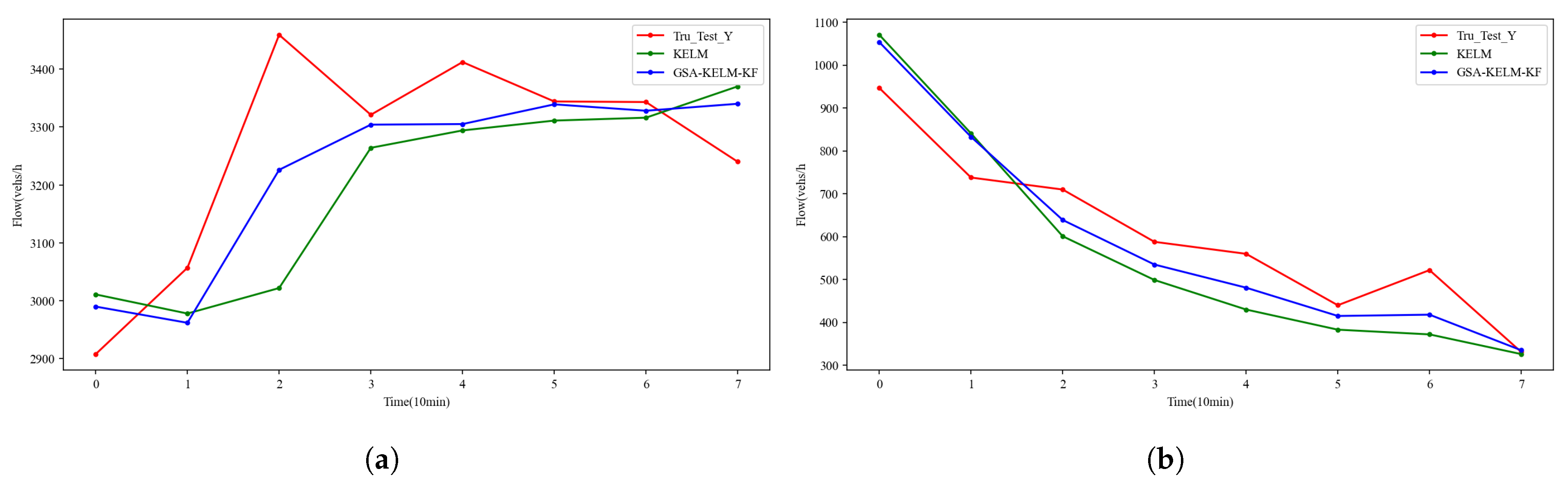
To further illustrate the performance of our model, we also conduct an intuitive comparison with KELM in two representative stages of morning peak passenger flow and nighttime low peak passenger flow in dataset A4.

In Figure 5a, the morning peak traffic flow ranges from 2900 to 3500 vehicles per hour. Traffic flow fluctuates greatly during this stage, and it is difficult for KELM to capture these rapid fluctuations. In this case, our GSA-KELM-KF prevents KELM from falling behind, effectively mitigating the shortcomings of sudden performance drops due to drastic traffic changes. This is extremely important in intelligent transportation systems and is a key issue in traffic management and traffic information release.

In Figure 5b, traffic flow gradually decreases at night. In this case, the traffic flow dropped relatively smoothly from 1100 vehicles per hour to 300 vehicles per hour. In this case, our GSA-KELM-KF can predict this change more accurately, prevent KELM from overshooting, and achieve more reasonable predictions.

To sum up, our method has better performances than other state-of-the-art models.

To further confirm the effectiveness of the proposal in different short-term traffic flow prediction tasks, we also compare it with several extreme learning methods on the M25 highway dataset, as summarized in

Table 3. The ${RMSE}_s$ of traffic flow datasets from D1 to D6 and P on England $M25$ highway dataset.

Models	D1	D2	D3	D4	D5	D6	P
ELM	161.49	116.81	124.22	51.52	19.44	149.33	29.17
GA-ELM	101.31	110.74	118.90	48.99	18.55	145.18	28.18
KELM	96.04	107.26	112.96	48.47	18.25	138.29	25.93
GSA-KELM(ours)	95.73	106.33	110.90	47.82	17.57	132.02	25.43
GSA-KELM-KF(ours)	94.58	106.08	109.81	47.75	17.48	129.98	25.39

Bold indicates optimal value.

.

Due to the zero values of traffic flow at some time on the dataset, the criterion of MAPE is unsuitable as an evaluation criterion. Under the criterion of RMSE, the GSA-KELM-KE achieves the best representation effects on all datasets, whose results are $94.58$, $106.08$, $109.81$, $47.75$, $17.48$, $129.98$, and $25.39$ on the D1, D2, D3, D4, D5, D6, and P datasets, respectively. Compared with KELM, the RMSE of our GSA-KELM-KF decreases by $1.52\%$, $1.10\%$, $2.78\%$, $1.48\%$, $4.21\%$, $6.00\%$, and $2.08\%$. Similarly, the RMSE of GSA-KELM decreases by $0.32\%$, $0.86\%$, $1.82\%$, $1.34\%$, $3.72\%$, $4.53\%$, and $1.92\%$. 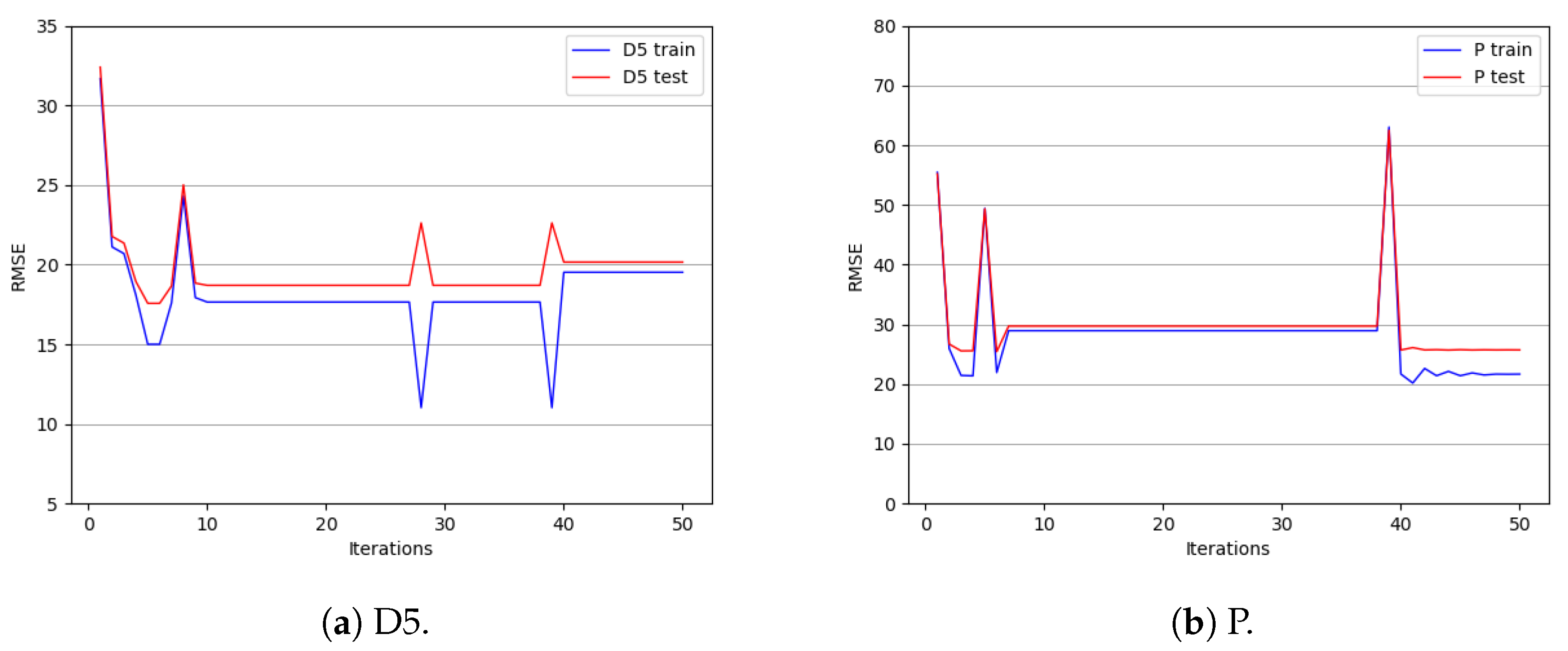Our GSA-KELM-KF model outperforms the ELM, KELM, and GSA-KELM on the England M25 highway dataset, showing the potential for accurate and reliable traffic flow prediction. 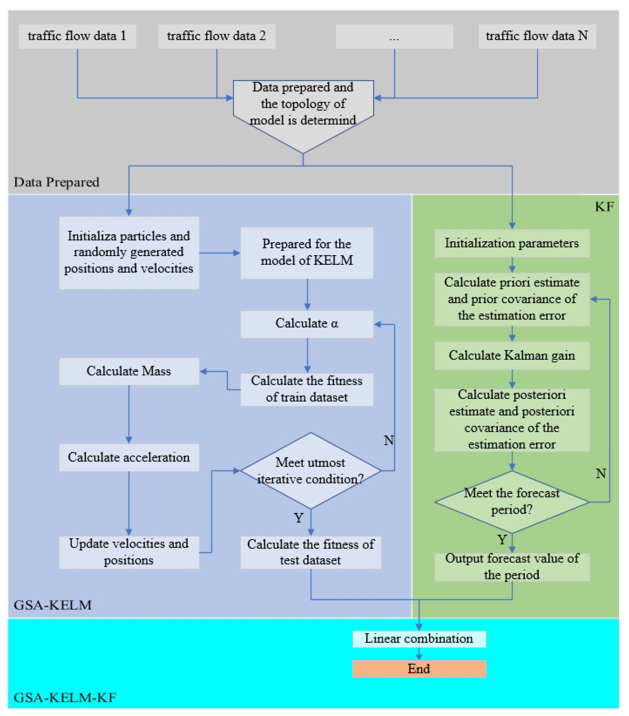It can be seen from Figure 6 that GSA can automatically break the convergence state after reaching a stable state to reach a new stable state, which provides the possibility of breaking away from the local optimal solution. When particles tend to converge, the state is broken by Equation (1).

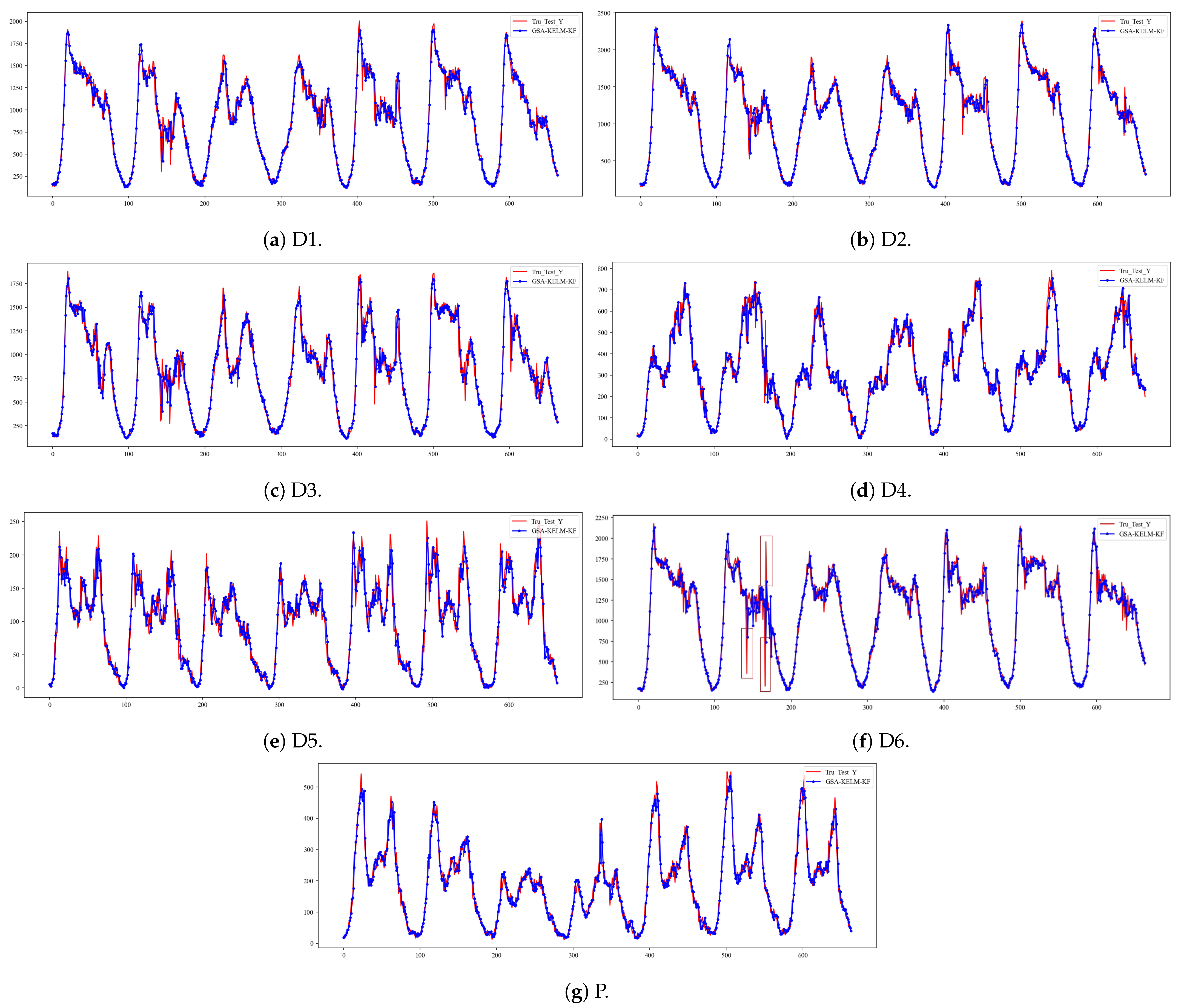
From Figure 7, our model also has a good fit on the England M25 highway dataset. Particularly, there are three outliers in Figure 7f, marked by red boxes. However, there is almost no fluctuation in the predicted values for outlier locations, indicating the strong robustness of our model.

3.5. Ablation Study

To verify the effectiveness of different components in our GSA-KELM-KF, we performed ablation experiments on the A1 and A4 datasets, as summarized in

Table 4. Component analysis of GSA-KELM-KF.

Dataset	Model and Variants	MAPE (%)	RMSE (vehs/h)
	GSA-KELM-KF	11.57	283.67
	GSA-KELM	11.63	284.93
A1	KELM-KF	11.61	284.40
	GSA-KELM-KF	11.20	216.78
	GSA-KELM	11.39	221.76
A4	KELM-KF	11.28	219.30

Bold indicates optimal value.

.

We compare the GSA-KELM-KF with the following several variants: (1) GSA-KELM, in which the variant removes the Kalman filter, which means we optimize KELM using the gravity search algorithm alone; (2) KELM-KF, in which the variant removes the gravity search algorithm, which means we use a grid traversal search algorithm.

From the experimental results, we can see that GSA-KELM-KF outperforms all ablation variants. Compared with the GSA-KELM, the MAPE and RMSE of GSA-KELM-KF on A4 decrease by $2.24\%$ and $1.66\%$, respectively. Correspondingly, the RMSE and MAPE of GSA-KELM-KF are $1.14\%$ and $0.71\%$ lower than those of KELM-KF, respectively. The above illustrates the effectiveness of the gravity search algorithm and Kalman filter components. The gravity search algorithm not only avoids manual traversal operations but also automatically searches for better solutions. The Kalman filter module can further reduce the impact of heavy-tail pulse noise interference.

In reality, traffic data always arrives chunk by chunk. We further divide the datasets of A1 and A4 into multiple mini-batches. For the convenience of experiments, we divide the datasets into several mini-batch sizes of 200. We use the first two batches of data for training and test the results on the third batch.

Table 5. The ${RMSE}_s$ and ${MAPE}_s$ of GSA-KELM-KF and KELM on A1 and A4 datasets.

Model	A1		A4
	RMSE (vehs/h)	MAPE (%)	RMSE (vehs/h)	MAPE (%)
KELM	288.54	11.37	223.78	9.65
GSA-KELM-KF	278.24	10.76	220.57	9.40

Bold indicates optimal value.

shows that GSA-KELM-KF achieves real-time prediction. In Figure 8, it shows excellent fitting effects. Overall, these findings suggest that our GSA-KELM-KF has promising potential in real-time traffic flow prediction applications.

4. Conclusions

In this paper, we propose a new KELM-based model (GSA-KELM-KF) for short-term traffic flow prediction. Our GSA-KELM-KF achieves the best performance in two real-world datasets, is insensitive to outliers, and exhibits strong robustness. Our model also has good fitting results on small batch data sets and has good application prospects in future work. Our model also has good fitting results on small-batch data sets. At the same time, the proposed method has some limitations. The basic datasets used in the article to train the traffic flow prediction model are relatively simple and come from highways. The application of more diverse traffic scenarios such as urban main roads will be included in our future research scope. We will also explore using additional data sources such as weather.