Stochastic Simulations of Casual Groups

Abstract

Free-forming or casual groups are groups in which individuals are in face-to-face interactions and are free to maintain or terminate contact with one another, such as clusters of people at a cocktail party, play groups in a children’s playground or shopping groups in a mall. Stochastic models of casual groups assume that group sizes are the products of natural processes by which groups acquire and lose members. The size distributions predicted by these models have been the object of controversy since their derivation in the 1960s because of the neglect of fluctuations around the mean values of random variables that characterize a collection of groups. Here, we check the validity of these mean-field approximations using an exact stochastic simulation algorithm to study the processes of the acquisition and loss of group members. In addition, we consider the situation where the appeal of a group of size i to isolates is proportional to $i^{\alpha }$. We find that, for $\alpha \le 1$, the mean-field approximation fits the equilibrium simulation results very well, even for a relatively small population size N. However, for $\alpha >1$, this approximation scheme fails to provide a coherent description of the distribution of group sizes. We find a discontinuous phase transition at ${\alpha }_c>1$ that separates the regime where the variance of the group size does not depend on N from the regime where it grows linearly with N. In the latter regime, the system is composed of a single large group that coexists with a large number of isolates. Hence, the same underlying acquisition-and-loss process can explain the existence of small, temporary casual groups and of large, stable social groups.

1. Introduction

Finding and explaining patterns in the ebb and flow of people in a public gathering have been challenging tasks for the mathematically inclined social scientist [1,2]. People constantly join and leave groups, so at any moment, the gathering appears as a collection of social clusters. The stochastic models proposed in the 1960s to explain the size distribution of these free-forming or casual groups ignore any prior knowledge of the individuals present in the gathering and use only a couple of parameters to represent people’s average tendencies to join and leave groups [3,4]. Here, we evaluate the suitability of these models to reproduce the empirical size distribution of casual groups.

In fact, the equilibrium group-size distributions resulting from these null models, viz., the zero-truncated Poisson distribution and the logarithmic distribution, well describe the observed size distributions of collections of small groups, such as pedestrians on a sidewalk, playgroups in a playground and shopping groups [3]. However, these distributions were derived using a mean-field approximation to solve equations for the expected number of groups of a given size, which prompted the criticism that they were not actual outcomes of the models but artifacts of the approximation scheme [4,5,6]. Here, we attempt to settle this long-standing (and likely forgotten) issue using Gillespie’s stochastic algorithm to exactly simulate the group dynamics [7,8].

In addition, we extend the null models proposed in the 1960s to consider the situation where the appeal of a group of size i to isolates (i.e., individuals who are not members of any group) is proportional to $i^{\alpha }$, where $\alpha \in (-\infty ,\infty )$ is the attractiveness exponent. Large negative values of $\alpha$ describe situations where a predominance of couples and isolates is expected, whereas large positive values of $\alpha$ foster the formation of a single large group that coexists with isolates. In time, the truncated Poisson distribution is obtained for $\alpha =0$ [3], and the logarithmic distribution is obtained for $\alpha =1$ [4], which have been the only cases studied so far. The stochastic simulations of the group dynamics indicate that the mean-field approximation yields the exact results for $\alpha \le 1$ and a large population size N. However, the approximation fails for $\alpha >1$ since it violates the fixed-population constraint.

The variation in the attractiveness exponent $\alpha$ allows the modeling of collections of small, temporary groups as well as of large, stable groups. We find that these two scenarios are separated by a discontinuous phase transition at $\alpha ={\alpha }_c>1$. The probability of observing large groups vanishes exponentially with increasing group size i for $\alpha <{\alpha }_c$. For $\alpha >{\alpha }_c$, the probability mass function concentrates around $i=1$ and $i=N-n_1$, where $n_1$ is the number of isolates. Hence, the acquisition-and-loss process of group dynamics does not produce a power-law decay for the probability of finding large groups observed in face-to-face interaction networks [9]. Long-tailed group-size distributions are outputs of agent-based models where the individuals are ascribed distinct degrees of attractiveness [10,11], so it seems that some knowledge of the individuals present in the gathering is necessary to produce these power-law distributions. In fact, the natural tendency of people to gravitate toward others who share similar interests or backgrounds is an important factor in explaining the formation of social groups [12,13,14]. Nevertheless, it is noteworthy that the stochastic null models can explain the empirical size distribution of collections of small groups.

A more recent and fruitful approach to the characterization of social groups or, more precisely, social networks—networks of friends or other acquaintances—is based on the complex networks framework [15]. In particular, a group of individuals (nodes) with a high density of internal links but with a comparatively lower density of external links is called a community [16,17]. Communities are ubiquitous in social and biological systems and are believed to represent real social groupings assembled by interest or background. We note that, although there are a variety of public repositories of animal social networks (see, e.g., [18,19]), the detection of communities in the real world as well as in artificial networks is a challenging computational task [20,21]. From an evolutionary perspective, the community organization of social networks is considered optimal if it boosts communication and decision making at the group level while keeping a minimum number of connections between individuals [22,23]. However, social network communities are relatively stable groups and thus are not good models for fleeting casual groups, which can be described by the less popular face-to-face interaction networks [24].

The rest of this paper is organized as follows: In Section 2, we describe the group dynamics and derive the exact equations for the expected number of groups of a given size. In Section 3, we present a brief overview of Gillespie’s algorithm and study the group dynamics using this stochastic simulation algorithm. In Section 4, we solve the equations derived in Section 2 for the equilibrium regime using the mean-field approximation and present explicit analytical expressions for the cases $\alpha \to -\infty$, $\alpha =0$ and $\alpha =1$, which are then compared with the simulation results. In Section 5, we study the equilibrium regime for $\alpha >1$ using stochastic simulations and show that in the limit $N\to \infty$, there is a discontinuous phase transition separating the scenarios where the variance of the group size is finite and where it diverges linearly with increasing N. Finally, in Section 6, we review our main results and present some concluding remarks.

2. The Model

We consider a fixed number of individuals N that organize themselves into a variable number of groups of size $i=1,\dots ,N$ in a closed system. We denote by $n_i$ the number of groups of size i at time t. These random variables satisfy the constraint ${\sum }_{i=1}^{N}i{n}_i=N$ and determine the total number of groups in the system, viz., ${\sum }_{i=1}^N{n}_i=M$, which is also a random variable. The processes of joining and leaving the groups are as follows.

Each individual in a group of size $i>1$ has a probability $\mu \delta t$ of leaving the group during the time interval $\delta t$. When an individual leaves a group, it becomes an isolate, i.e., a group of size $i=1$. An isolate has a probability $\lambda \delta t$ of joining a group (including other isolates) in the time interval $\delta t$.

We assume that the attractiveness of a group of size i to isolates is proportional to $i^{\alpha }$. The case $\alpha =0$ describes the situation where isolates join any group in the system at the same rate, whatever its size [3]. For $\alpha >0$, we have a contagious scenario that favors the formation of large groups [4], whereas, for $\alpha <0$, we have an aversion scenario that disfavors the formation of groups. In the 1960s, approximate analytical expressions for the expected values of $n_i$ were derived for the cases $\alpha =0$ and $\alpha =1$ only [3,4].

The understanding of the processes by which groups acquire and lose individuals is facilitated if we write down the conditional expected values of the random variables $n_i(t+\delta t)$ given that the system is in the state $\overrightarrow{n}\left(t\right)=\left(n_1\left(t\right),\dots ,n_N\left(t\right)\right)$ at time t. Let us begin with the conditional expectation of the number of isolates,

$$\mathbb{E}\left[n_1(t+\delta t)|\overrightarrow{n}\left(t\right)\right]=n_1+\mu \delta t\left(2n_2\right)+\mu \delta t(N-n_1)-\lambda \delta t{n}_1\frac{N_{\alpha }-n_1}{N_{\alpha }-1}-2\lambda \delta t{n}_1\frac{n_1-1}{N_{\alpha }-1},$$

(1)

where we have omitted the dependence of the variables $n_i\left(t\right)$ on t that appear on the right-hand side (RHS) of the equation. In addition, we have introduced the notation

$$N_{\alpha }\left(t\right)=1^{\alpha }{n}_1\left(t\right)+2^{\alpha }{n}_2\left(t\right)+\dots +N^{\alpha }{n}_N\left(t\right),$$

(2)

so that $N_0\left(t\right)=M\left(t\right)$ and $N_1\left(t\right)=N$. The third term on the RHS of Equation (1) takes into account the fact that any individual who is not isolated may become an isolate with a probability of $\mu \delta t$. The second term corrects the third term by reckoning with the fact that whenever an individual leaves a group of two individuals, two isolates are created. The fourth term on the RHS of Equation (1) accounts for the event that an isolate joins any group with $i>1$ individuals, whereas the fifth term accounts for the aggregation of two isolates.

Next, we consider the conditional expectation of the number of couples, viz.,

$$\mathbb{E}\left[n_2(t+\delta t)|\overrightarrow{n}\left(t\right)\right]=n_2+3\mu \delta t{n}_3-2\mu \delta t{n}_2-\lambda \delta t{n}_1\frac{2^{\alpha }{n}_2}{N_{\alpha }-1}+\lambda \delta t{n}_1\frac{n_1-1}{N_{\alpha }-1}.$$

(3)

The second and third terms on the RHS of Equation (3) account for the facts that a group of two individuals is created when an individual leaves a group of three individuals, and it is destroyed when an individual leaves a group of two individuals. The fourth term accounts for the event that isolates attracted by groups of two individuals produce groups of three individuals, and the fifth term accounts for the joining of two isolates to produce a group of two individuals.

For groups with $i=3,\dots ,N$ individuals, we can write the general expression

$$\mathbb{E}\left[n_i(t+\delta t)|\overrightarrow{n}\left(t\right)\right]=n_i+(i+1)\mu \delta t{n}_{i+1}-i\mu \delta t{n}_i-\lambda \delta t{n}_1\frac{i^{\alpha }{n}_i}{N_{\alpha }-1}+\lambda \delta t{n}_1\frac{{(i-1)}^{\alpha }{n}_{i-1}}{N_{\alpha }-1},$$

(4)

with $n_{N+1}\equiv 0$. The interpretation of the terms in this equation follows straightforwardly from the interpretations of the terms in Equations (1) and (3).

We stress that Equations (1), (3) and (4) for the conditional expectations of $n_i(t+\delta t),i=1,\dots ,N$ are exact. Adding these equations yields the conditional expectation for the number of groups,

$$\mathbb{E}\left[M(t+\delta t)|\overrightarrow{n}\left(t\right)\right]=M\left(t\right)+\mu \delta t[N-n_1\left(t\right)]-\lambda \delta t{n}_1\left(t\right),$$

(5)

from which we can see that the isolates play a key role in driving the casual group dynamics.

Averaging Equations (1), (3)–(5) over the states $\overrightarrow{n}\left(t\right)$ and taking the limit $\delta t\to 0$ yield

$$\begin{array}{ccc}\hfill \frac{d\langle n_1\rangle }{dt}& =& 2\mu \langle n_2\rangle +\mu (N-\langle n_1\rangle )-\lambda \mathbb{E}\left[\frac{n_1(N_{\alpha }-n_1)}{N_{\alpha }-1}\right]-2\lambda \mathbb{E}\left[\frac{n_1(n_1-1)}{N_{\alpha }-1}\right],\hfill \end{array}$$

(6)

$$\begin{array}{ccc}\hfill \frac{d\langle n_2\rangle }{dt}& =& 3\mu \langle n_3\rangle -2\mu \langle n_2\rangle -2^{\alpha }\lambda \mathbb{E}\left[\frac{n_1{n}_2}{N_{\alpha }-1}\right]+\lambda \mathbb{E}\left[\frac{n_1(n_1-1)}{N_{\alpha }-1}\right],\hfill \end{array}$$

(7)

$$\begin{array}{ccc}\hfill \frac{d\langle n_i\rangle }{dt}& =& (i+1)\mu \langle n_{i+1}\rangle -i\mu \langle n_i\rangle -i^{\alpha }\lambda \mathbb{E}\left[\frac{n_1{n}_i}{N_{\alpha }-1}\right]+{(i-1)}^{\alpha }\lambda \mathbb{E}\left[\frac{n_1{n}_{i-1}}{N_{\alpha }-1}\right]\hfill \end{array}$$

(8)

for $i=2,\dots ,N$, and

$$\frac{d\langle M\rangle }{dt}=\mu N+(\lambda -\mu )\langle n_1\rangle ,$$

(9)

where $\langle n_{N+1}\rangle \equiv 0$, and we have introduced the notation $\langle n_i\left(t\right)\rangle \equiv \mathbb{E}\left[n_i\left(t\right)\right]$. We note that by rescaling the time $\tau =\mu t$, these equations depend on the aggregation and disaggregation rates only through their ratio,

$$\kappa \equiv \frac{\lambda }{\mu }.$$

(10)

Of course, Equations (6)–(8) do not form a closed set of equations since there are quantities (e.g., $\mathbb{E}[n_1^2/(N_{\alpha }-1)]$) that are left undefined. Somewhat surprisingly, however, in the equilibrium regime, i.e., $d\langle n_i\rangle /dt=0$ for $i=1,\dots ,N$, Equation (9) yields the exact mean number of isolates,

$${\langle n_1\rangle }_{eq}=\frac{N}{1+\kappa },$$

(11)

which does not depend on the attractiveness exponent $\alpha$.

3. The Gillespie Algorithm

Here, we offer a brief overview of Gillespie’s algorithm for simulating continuous-time stochastic models [7,8]. In the time interval $\delta t$, the probability that aggregation occurs is $\lambda n_1\left(t\right)\delta t$, and the probability that an individual leaves a group is $\mu [N-n_1\left(t\right)]\delta t$. Since these two events decrease and increase the number of groups by one unity, respectively, their probabilities appear on the RHS of Equation (5). Given the state $\overrightarrow{n}\left(t\right)$ at time t, the probability that the next event will occur in the infinitesimal time interval $(t+t^{\prime },t+t^{\prime }+\delta t^{\prime })$ is $P\left(t^{\prime }\right)\delta t^{\prime }$, where $P\left(t^{\prime }\right)$ is the exponential distribution,

$$P\left(t^{\prime }\right)=\upsilon exp\left(-t^{\prime }\upsilon \right).$$

(12)

and

$$\upsilon =\mu N+(\lambda -\mu )n_1\left(t\right)$$

(13)

is the total rate of events. The event that occurs in the time interval $(t+t^{\prime },t+t^{\prime }+\delta t^{\prime })$ is an aggregation with a probability $\lambda n_1\left(t\right)/\upsilon$ and a disaggregation with a probability $\mu [N-n_1\left(t\right)]/\upsilon$. In the case that aggregation occurs, there are two possibilities: an isolate can join a group of size $i>1$, which is an event that happens with a probability

$$\frac{i^{\alpha }{n}_i\left(t\right)}{n_1\left(t\right)-1+2^{\alpha }{n}_2\left(t\right)+\dots +N^{\alpha }{n}_N\left(t\right)},$$

(14)

or two isolates can join together to form a couple, which has a probability

$$\frac{n_1\left(t\right)-1}{n_1\left(t\right)-1+2^{\alpha }{n}_2\left(t\right)+\dots +N^{\alpha }{n}_N\left(t\right)}.$$

(15)

In the case that disaggregation occurs in the time interval $(t+t^{\prime },t+t^{\prime }+\delta t^{\prime }),$ a single individual leaves a group of size $i>1$, which is an event that happens with a probability

$$\frac{i{n}_i\left(t\right)}{2n_2\left(t\right)+\dots +N{n}_N\left(t\right)}=\frac{i{n}_i\left(t\right)}{N-n_1\left(t\right)}.$$

(16)

In sum, given the state of the system $\overrightarrow{n}\left(t\right)$ at time t, the stochastic simulation of the casual-group model begins with the choice of the time $t^{\prime }$ when the next event will occur using the distribution in (12), followed by the choice of the type of event—aggregation with a probability $\lambda n_1\left(t\right)/\upsilon$ and disaggregation with a probability $\mu [N-n_1\left(t\right)]/\upsilon$. Finally, the specific aggregation and disaggregation events are chosen with probabilities given by Equations (14)–(16). We note that, with the exception of the determination of the time of the next event, the aggregation and disaggregation rates always appear in the form of the ratio $\lambda /\mu$. This numerical algorithm produces the exact trajectories of the states $\overrightarrow{n}\left(t\right)$, which, when properly averaged over many independent runs, offers the only way to verify the validity of the approximation schemes used to solve high-dimensional master equations [7,8].

Here, we use the bracket notation $\langle \dots \rangle$ to indicate the average over independent runs. In fact, because the number of runs is very large (typically ${10}^6$), we can safely equate the average over independent runs to the expected values of the random variables $n_1\left(t\right),\dots ,n_N\left(t\right)$, hence the choice of the same bracket notation used in Section 2.

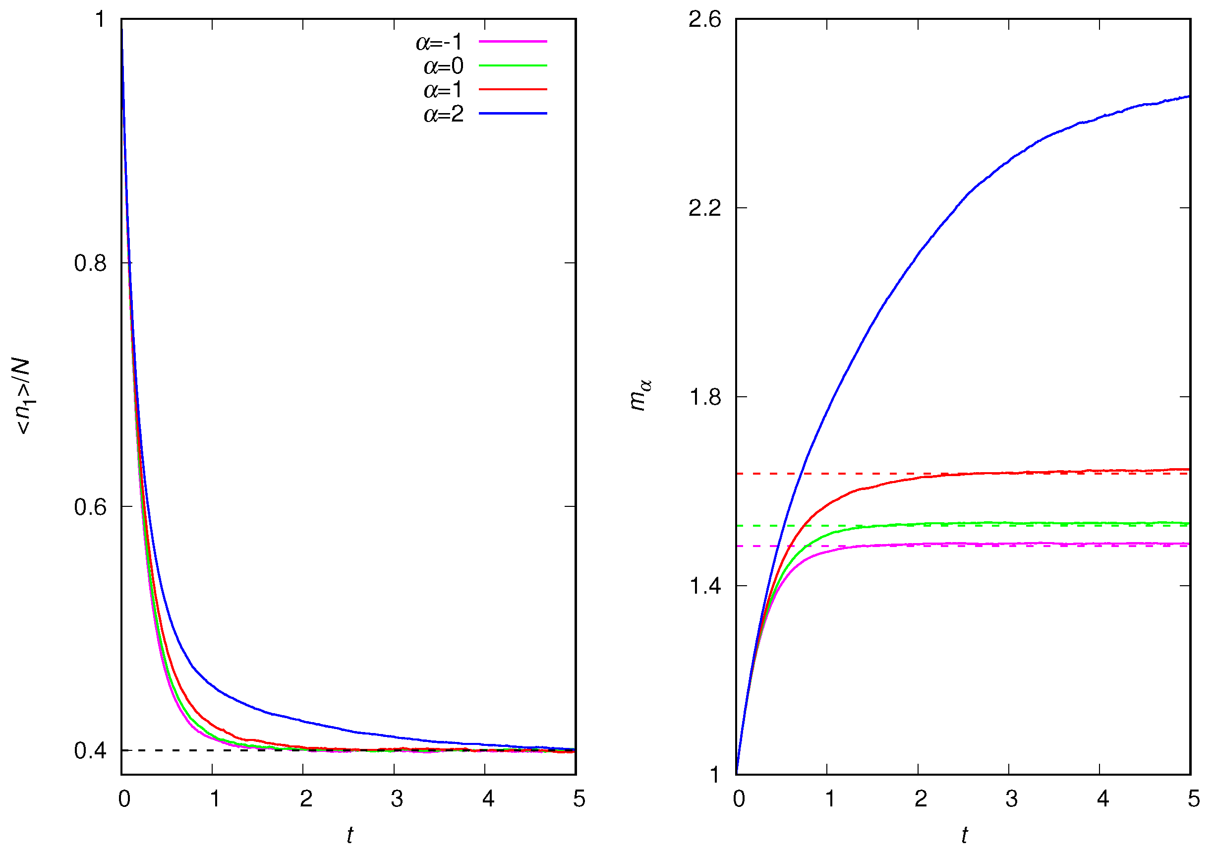
Figure 1 shows the time evolution of the mean density of isolates, $\langle n_1\left(t\right)\rangle /N$, and the mean number of individuals per group $m_{\alpha }\equiv \langle N/M\left(t\right)\rangle$ for different values of the attractiveness exponent $\alpha$. At time $t=0$, all N individuals are isolates (i.e., $n_1\left(0\right)=N$ and $n_i\left(0\right)=0,i>1$). Interestingly, although the mean density of isolates does not depend on $\alpha$ in the equilibrium regime, as shown in Equation (11), the transient regime is affected by the attractiveness exponent: the increase in $\alpha$ favors the production of isolates. This is so because $\alpha >0$ hinders the formation of couples, which requires the annihilation of two isolates, whereas the formation of groups of size $i>2$ requires the annihilation of only one isolate. In addition, an increase in $\alpha$ increases the transient period, as well as the mean size of the groups.

Figure 2 shows the effect of the population size N on the density of isolates and on the mean group size for $\alpha =0$. The results are qualitatively similar to other values of the attractiveness exponent. We note the remarkable unresponsiveness of the density of isolates to changes in N. In fact, although the decrease in N results in a reduction in the rate of events $\upsilon$, given by Equation (13), the effect of a single event on the density of isolates is enhanced. These two effects compensate for each other, resulting in a system size invariance of $\langle n_1\left(t\right)\rangle /N$. However, the mean group size decreases with increasing N and converges very rapidly to the infinite system size limit. For $\alpha \le 1$, this limit is described very well by the analytical approximation for the equilibrium solutions of Equations (6)–(8) that we will derive in the next section.

4. Analytical Approximation for the Equilibrium Regime

Here, we derive the controversial approximate analytical results for the expectations $\mathbb{E}\left[n_i\left(t\right)\right]\equiv \langle n_i\left(t\right)\rangle$ that motivated the present contribution [4,5,6]. In the following, we will focus only on the equilibrium regime, i.e., $d\langle n_i\rangle /dt=0$ for $i=1,\dots ,N$. To solve the equilibrium equations for ${\langle n_i\rangle }_{eq}$ with $i>1$, we make the assumption

$$\mathbb{E}\left[f\left(n_1,\dots ,n_N\right)\right]=f\left({\langle n_1\rangle }_{eq},\dots ,{\langle n_N\rangle }_{eq}\right),$$

(17)

where f is an arbitrary rational function. Such a strong assumption is valid if the random variables $n_i$ are self-averaging, i.e., $n_i/N\to {\langle n_i\rangle }_{eq}/N$ for all i in the limit $N\to \infty$. This neglect of fluctuations is the basis of the popular mean-field approximation of statistical physics [25]. With this assumption, we can easily write ${\langle n_i\rangle }_{eq}$ for $i>1$ in terms of ${\langle n_1\rangle }_{eq}$ and ${\langle N_{\alpha }\rangle }_{eq}$,

$${\langle n_i\rangle }_{eq}=\frac{{[(i-1)!]}^{\alpha -1}}{i}{\left[\kappa \frac{{\langle n_1\rangle }_{eq}}{{\langle N_{\alpha }\rangle }_{eq}-1}\right]}^{i-1}({\langle n_1\rangle }_{eq}-1)$$

(18)

where ${\langle N_{\alpha }\rangle }_{eq}={\sum }_{i=1}^N{i}^{\alpha }{\langle n_i\rangle }_{eq}$, and ${\langle n_1\rangle }_{eq}$ is given by Equation (11). These equations must be solved self-consistently: for an arbitrary value of ${\langle N_{\alpha }\rangle }_{eq}$, we calculate ${\langle n_i\rangle }_{eq}$ for $i>1$, which we then use to update the estimate of ${\langle N_{\alpha }\rangle }_{eq}$. The process is repeated until convergence. At this point, we can already see that the assumption in (17) leads to nonphysical results for $\kappa >N-1$, where ${\langle n_1\rangle }_{eq}<1$ (see Equation (11)), since it implies ${\langle n_i\rangle }_{eq}<0$ for $i>1$. This breakdown of the mean-field approximation is expected because a necessary condition for the self-averaging property to hold is that ${\langle n_1\rangle }_{eq}\gg 1$ for large N.

In addition, and more importantly, Equation (18) holds for $\alpha \le 1$ only. Although for finite N, the self-consistent strategy yields a solution for any value of $\alpha$, in which ${\langle N_{\alpha }\rangle }_{eq}$ scales with $N^{\alpha }$, the solution does not satisfy the constraint ${\sum }_{i=1}^{N}i{\langle n_i\rangle }_{eq}=N$ for $\alpha >1$. The reason is that Equation (18) yields a non-negligible value for ${\langle n_N\rangle }_{eq}$, resulting in a net flow of individuals to nonphysical group sizes and the consequent violation of the constant-population-size constraint. This effect is negligible for $\alpha \le 1$ because ${\langle n_N\rangle }_{eq}$ is vanishingly small (provided that N is not too small), so the flow of individuals to nonphysical regions is inconsequential. We stress that the exact simulations of the group dynamics result in negligible values of ${\langle n_N\rangle }_{eq}$ for any $\alpha$, as we will show in Section 5.

A relevant quantity that is usually observed in empirical investigations [1,2,3] is the mean fraction of groups of size $i=1,\dots ,N$ at equilibrium, defined as

$$p_i={\langle \frac{n_i}{M}\rangle }_{eq}\approx \frac{{\langle n_i\rangle }_{eq}}{{\langle M\rangle }_{eq}},$$

(19)

where the approximation is justified by the assumption in (17). Of course, $p_i$ can be interpreted as the probability of observing a group of size i. It is interesting that empirical studies typically clump together groups of the same size that are observed on many different occasions (e.g., pedestrians on a sidewalk during Spring mornings in Eugene, Oregon [3]), so they report the total number of observations of groups of a given size. Summing over the different sizes yields the total number of groups observed. Hence, the ratio between the two averages ${\langle n_i\rangle }_{eq}/{\langle M\rangle }_{eq}$ is actually the correct measure to describe the empirical results. However, in stochastic simulations, we calculate the ratios $n_i/M$ for each run and then average the results over the many independent runs, so we measure ${\langle n_i/M\rangle }_{eq}$.

In the following, we present explicit analytical expressions of $p_i$ for $\alpha =0$, $\alpha =1$ and the limit $\alpha \to -\infty$. In addition, we present the numerical solution of Equation (18) obtained with the self-consistent method for general $\alpha \le 1$.

4.1. Case $\alpha =0$

In this case, ${\langle N_{\alpha }\rangle }_{eq}={\langle M\rangle }_{eq}$, and Equation (18) reduces to

$${\langle n_i\rangle }_{eq}=\frac{1}{i!}{\left[\kappa \frac{{\langle n_1\rangle }_{eq}}{{\langle M\rangle }_{eq}-1}\right]}^{i-1}({\langle n_1\rangle }_{eq}-1)$$

(20)

for $i>1$, with

$$\begin{array}{ccc}\hfill {\langle M\rangle }_{eq}& =& \sum _{i=1}^N{\langle n_i\rangle }_{eq}\hfill \\ & \approx & 1+\frac{1}{\kappa }({\langle M\rangle }_{eq}-1)(1-\frac{1}{{\langle n_1\rangle }_{eq}})[exp\left(\kappa \frac{{\langle n_1\rangle }_{eq}}{{\langle M\rangle }_{eq}-1}\right)-1],\hfill \end{array}$$

(21)

from which we obtain an explicit expression for the mean number of groups in the equilibrium regime,

$${\langle M\rangle }_{eq}\approx \frac{\kappa }{1+\kappa }\frac{N}{ln(1+\kappa )}.$$

(22)

In deriving Equation (21), we have assumed that $N\to \infty$ in order to carry out the sum over the group sizes, whereas, in deriving Equation (22), we have assumed that ${\langle n_1\rangle }_{eq}$ is on the order of N, which means that $\kappa \ll N$. As already pointed out, these are the necessary conditions for the validity of the self-averaging property that underlies the mean-field approximation.

Hence,

$$p_i=\frac{1}{e^a-1}\frac{a^i}{i!},$$

(23)

where $a=ln(1+\kappa )$, which we identify as the zero-truncated Poisson distribution. Interestingly, this distribution fits a wide variety of data of small groups [3]. The mean and the variance of the group size are

$$m_0=\sum _{i=1}^{N}i{p}_i=(1+1/\kappa )ln(1+\kappa )$$

(24)

and

$${\sigma }_0^2=\left(1+1/\kappa \right)\left[ln(1+\kappa )+{ln}^2(1+\kappa )\right]-{\left(1+1/\kappa \right)}^2{ln}^2(1+\kappa ).$$

(25)

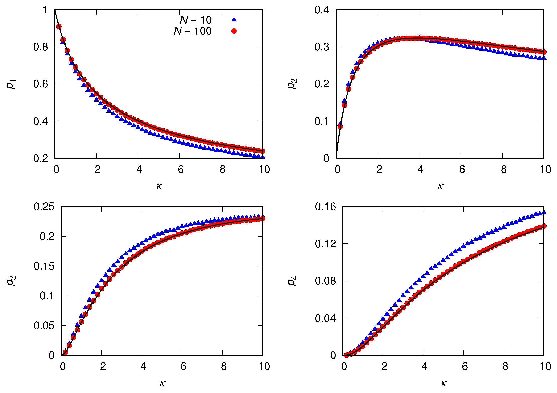
Figure 3 exhibits the comparison between the stochastic simulations and the truncated Poisson distribution (23) for $N=10$ and $N=100$. As expected, the mean-field approximation fails to describe the size distribution for $N=10$, but for $N=100$, its predictions are indistinguishable from the simulation results. This finding validates the use of that approximation, provided that the number of individuals is not too small.

4.2. Case $\alpha =1$

In this case, ${\langle N_{\alpha }\rangle }_{eq}=N$, and Equation (18) reduces to

$${\langle n_i\rangle }_{eq}=\frac{1}{i}{\left[\kappa \frac{{\langle n_1\rangle }_{eq}}{N-1}\right]}^{i-1}({\langle n_1\rangle }_{eq}-1)$$

(26)

with ${\langle n_1\rangle }_{eq}$ given in Equation (11). As before, assuming that $N\gg 1$ and ${\langle n_1\rangle }_{eq}\gg 1$, we obtain an explicit expression for the mean number of groups:

$${\langle M\rangle }_{eq}\approx N\frac{1}{\kappa }ln(1+\kappa ).$$

(27)

Thus, the fraction $p_i$ of groups of size $i>0$ is

$$p_i=\frac{1}{ln(1+\kappa )}\frac{1}{i}{\left(\frac{\kappa }{1+\kappa }\right)}^i,$$

(28)

which we identify as the logarithmic distribution used to model relative species abundance [26]. Hence, the mean group size is

$$m_1=\frac{\kappa }{ln(1+\kappa )}$$

(29)

and the variance of the group size is

$${\sigma }_1^2=\frac{-{\kappa }^2+\kappa (1+\kappa )ln(1+\kappa )}{{ln}^2(1+\kappa )}.$$

(30)

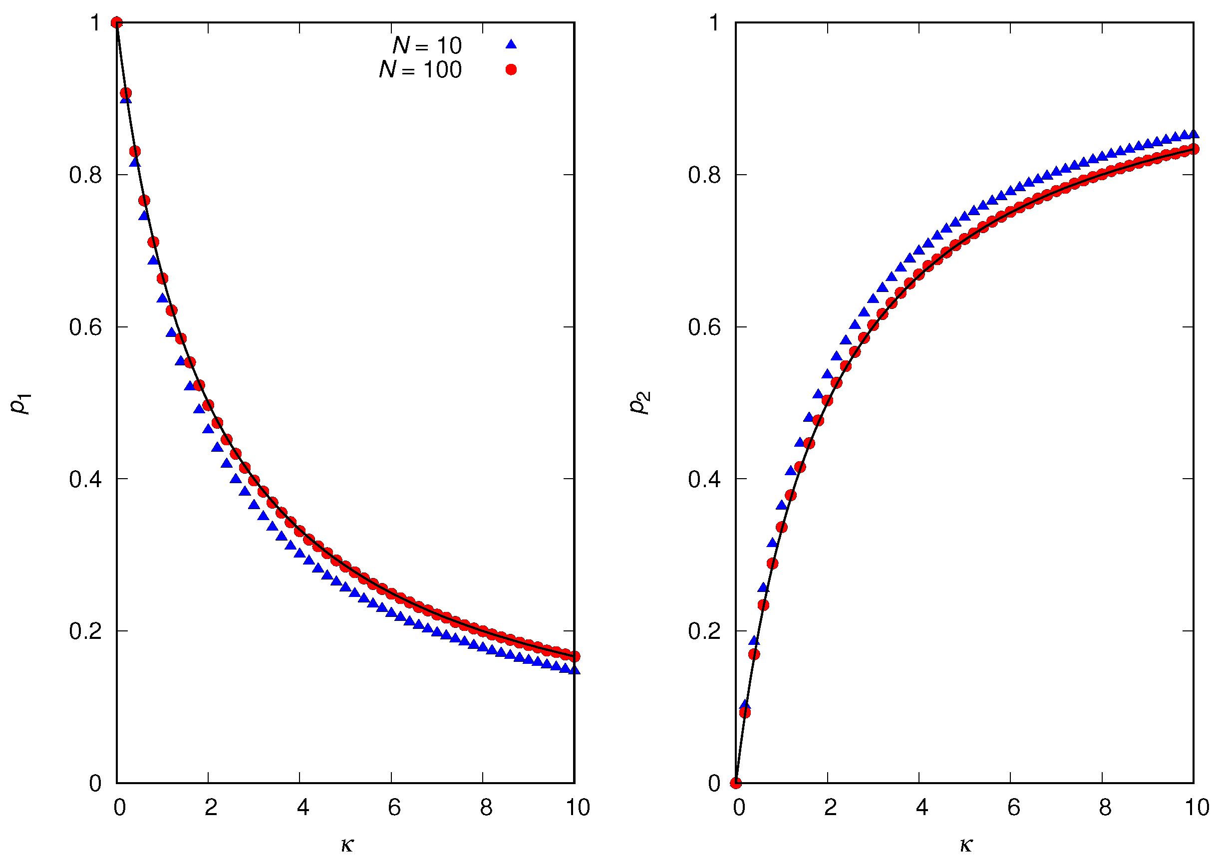
Figure 4 exhibits the comparison between the stochastic simulations and the logarithmic distribution (28) for $N=10$ and $N=100$. As before, the results validate the use of the mean-field approximation if the number of individuals is not too small.

4.3. The Limit $\alpha \to -\infty$

In the limit $\alpha \to -\infty$, we have ${\langle N_{-\infty }\rangle }_{eq}={\langle n_1\rangle }_{eq}$, ${\langle n_2\rangle }_{eq}=\kappa {\langle n_1\rangle }_{eq}/2$ and ${\langle n_i\rangle }_{eq}=0$ for $i>2$. Hence, the fraction of groups of size i is

$$\begin{array}{ccc}\hfill p_1& =& \frac{1}{1+\kappa /2}\hfill \end{array}$$

(31)

$$\begin{array}{ccc}\hfill p_2& =& \frac{\kappa /2}{1+\kappa /2}\hfill \end{array}$$

(32)

and $p_i=0$ for $i>2$. Figure 5 shows the simulation results for $N=10$ and $N=100$. We have verified that $p_i=0$ for $i>2$ in the simulations. As before, although the mean-field approximation fails for $N=10$, it yields the exact result for $N=100$.

The mean group size is

$$m_{-\infty }=\frac{1+\kappa }{1+\kappa /2}$$

(33)

and the variance of the group size is

$${\sigma }_{-\infty }^2=\frac{\kappa /2}{{(1+\kappa /2)}^2}.$$

(34)

The limit $\alpha \to -\infty$ is instructive because we can solve Equations (6)–(8) exactly for any value of $N>1$ using the fact that $i^{\alpha }\to 0$ for $i>1$. We find

$$\langle n_1\left(t\right)\rangle =\langle n_1\left(0\right)\rangle e^{-2(1+\kappa )\tau }+\frac{N}{1+\kappa }\left(1-e^{-2(1+\kappa )\tau }\right)$$

(35)

where $\tau =\mu t$. From this equation, we can easily obtain $\langle n_2\left(t\right)\rangle =(N-\langle n_1\left(t\right)\rangle )/2$ and $\langle M\left(t\right)\rangle =(N+\langle n_1\left(t\right)\rangle )/2$. The reason that Equations (31) and (32) are only approximate and thus fail to fit the data for $N=10$ in Figure 5 is that, although we can calculate $\langle n_1\rangle$ and $\langle M\rangle$ exactly for all $N>1$, we do not know how to calculate $p_1=\langle n_1/M\rangle$, which is the quantity measured in the simulations.

4.4. General $\alpha \le 1$

Except for the three cases discussed before, it is not possible to obtain explicit analytical expressions for ${\langle n_i\rangle }_{eq}$ because we cannot carry out the summation necessary to compute ${\langle N_{\alpha }\rangle }_{eq}$ in a closed form. However, the use of the self-consistent method allows us to easily obtain these quantities numerically. 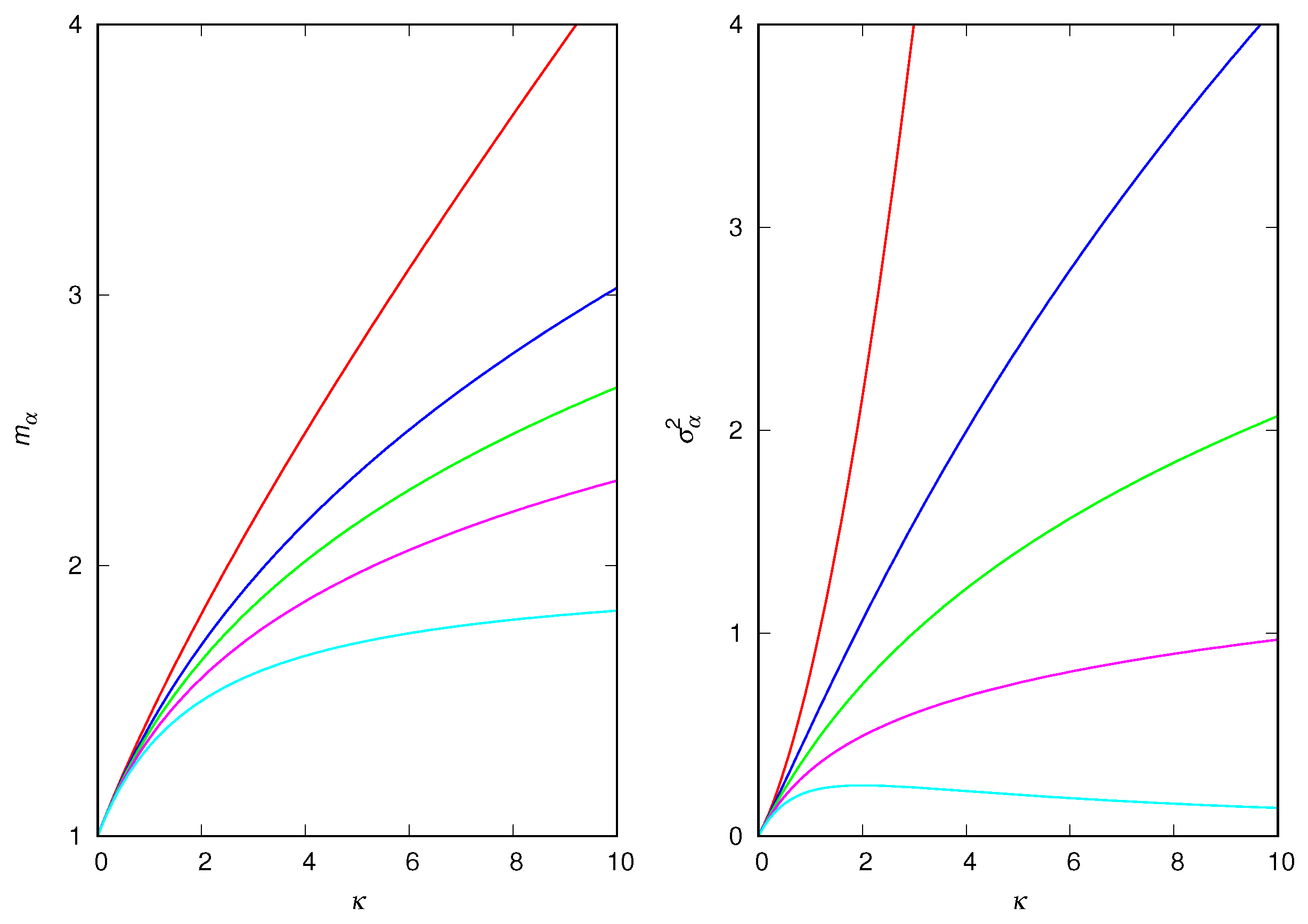Since we have already established that the mean-field approximation is very accurate, even for $N=100$, in Figure 6, we present only the approximate theoretical results for $m_{\alpha }$ and ${\sigma }_{\alpha }^2$.

As expected, decreasing the value of the attractiveness exponent decreases the mean and the variance of the group sizes. We note that these quantities have explicit analytical expressions in the cases $\alpha =0$ (Equations (24) and (25)), $\alpha =1$ (Equations (29) and (30)) and $\alpha \to -\infty$ (Equations (33) and (34)).

5. Equilibrium Regime for $\alpha >1$

This is by far the most interesting situation because of the complete failure of the mean-field approximation. As already pointed out, the reason is that the solution of Equation (18) violates the fixed-population constraint for $\alpha >1$. However, we can still obtain some useful analytical information by considering the limit of very large $\alpha$. In this limit, the system is composed of ${\langle n_1\rangle }_{eq}$ isolates and a single group of $N-{\langle n_1\rangle }_{eq}$ individuals on average. Hence, the mean number of groups is ${\langle M\rangle }_{eq}={\langle n_1\rangle }_{eq}+1$, and we have

$$m_{\infty }\approx \frac{{\langle n_1\rangle }_{eq}+(N-{\langle n_1\rangle }_{eq})}{{\langle n_1\rangle }_{eq}+1}\approx 1+\kappa$$

(36)

and

$${\sigma }_{\infty }^2\approx \frac{{\langle n_1\rangle }_{eq}+{(N-{\langle n_1\rangle }_{eq})}^2}{{\langle n_1\rangle }_{eq}+1}-m_{\infty }^2\approx N\frac{{\kappa }^2}{1+\kappa },$$

(37)

so that the mean group size is finite, but the variance diverges in the limit $N\to \infty$. The mean size of the large group is

$$N-{\langle n_1\rangle }_{eq}=\frac{N\kappa }{1+\kappa }.$$

(38)

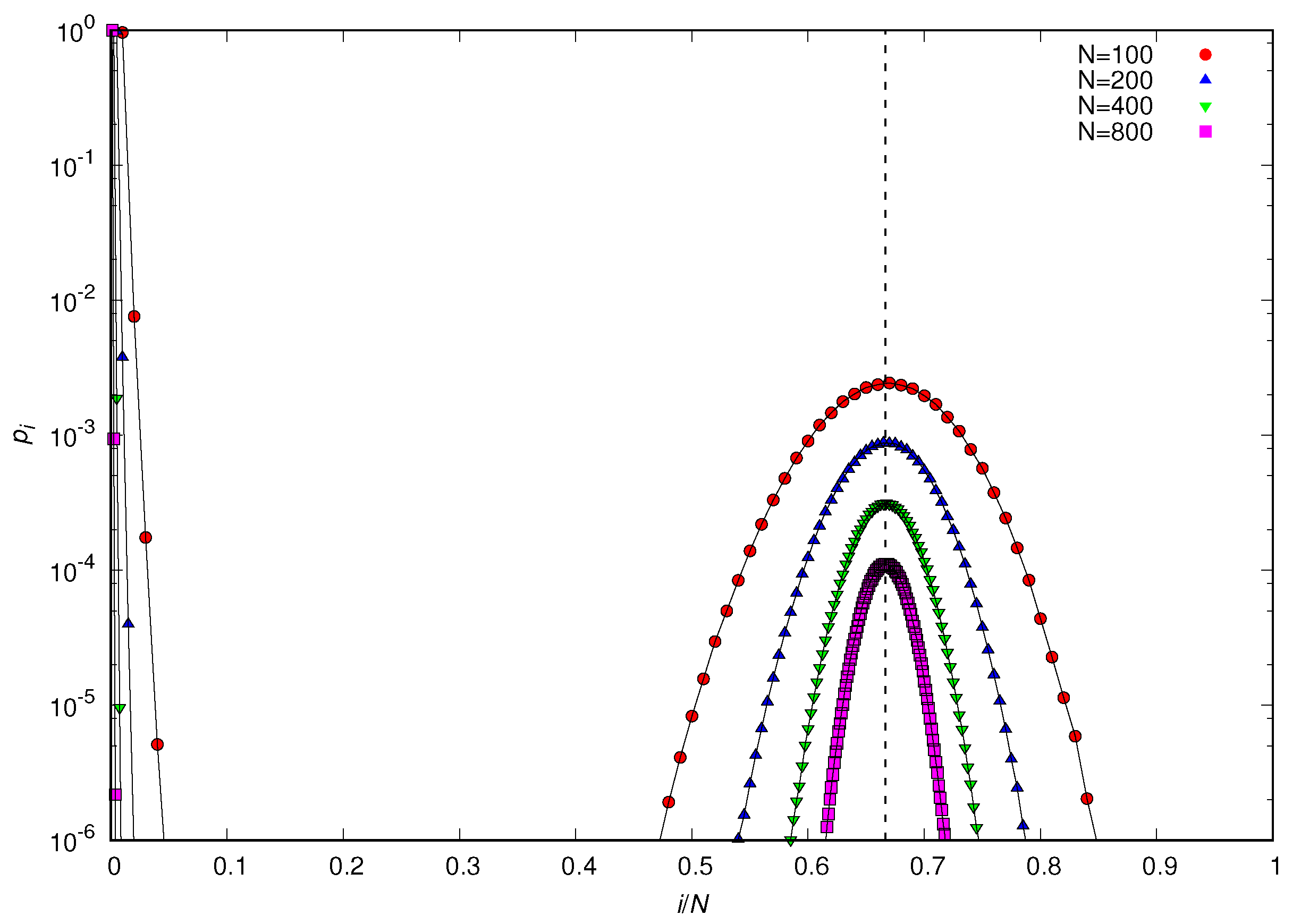
Interestingly, Figure 7 shows that this scenario—a single large group coexisting with isolates—describes the case $\alpha =2$ very well for large N. Figure 8 corroborates this finding by showing that $p_i$ tends to a bimodal distribution characterized by sharp peaks at $i=1$ and $i=N-n_1$ in the limit of large N. In addition, this figure shows that $p_N$ (or ${\langle n_N\rangle }_{eq}$) is negligibly small for $\alpha >1$, in disagreement with the prediction (17) of the mean-field approximation.

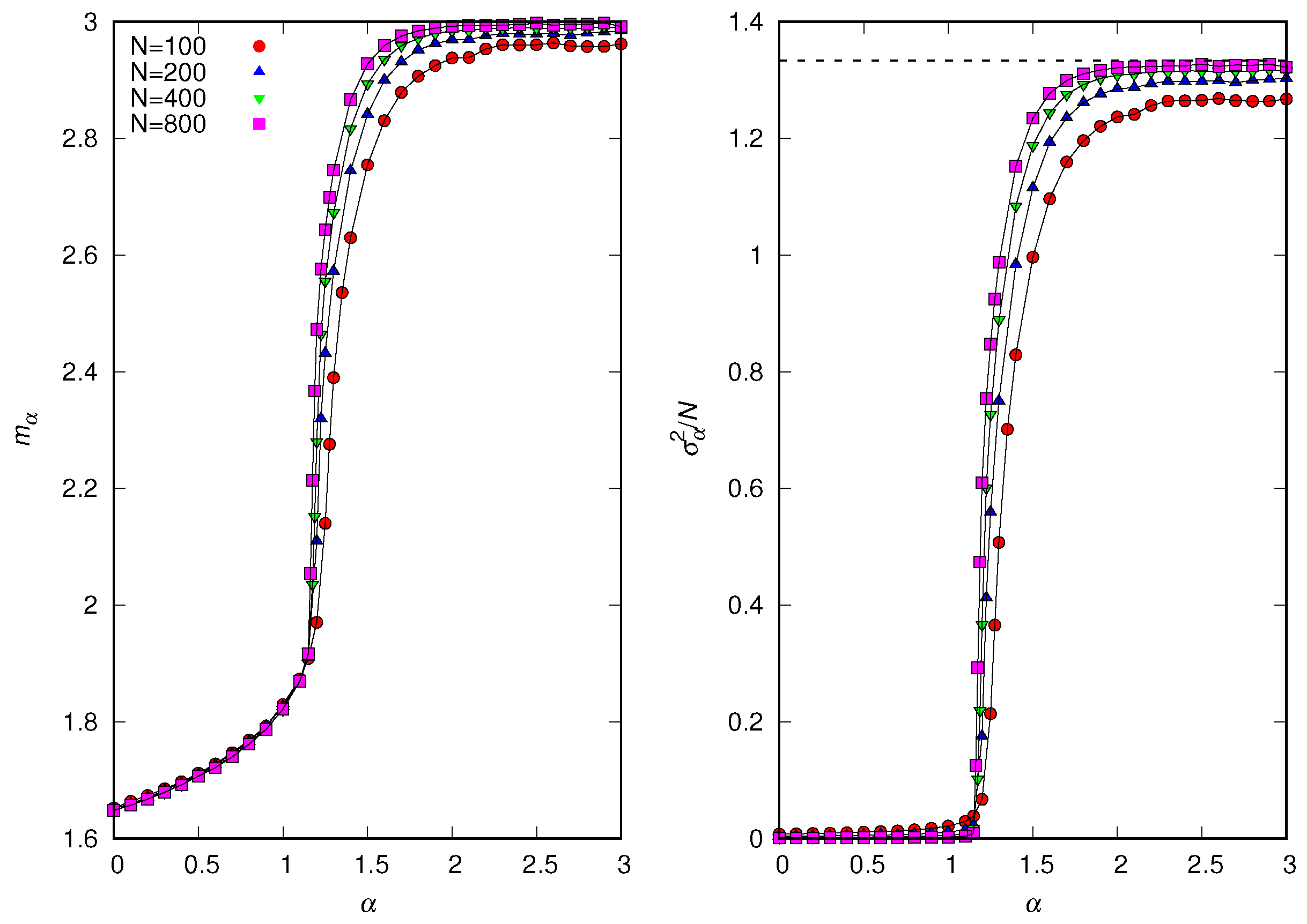
In order to better understand the transition between the equilibrium regime characterized by a finite variance ${\sigma }_{\alpha }^2$ and the regime where ${\sigma }_{\alpha }^2$ diverges linearly with N as $N\to \infty$, in Figure 9, we show the influence of the attractiveness exponent $\alpha$ on $m_{\alpha }$ and ${\sigma }_{\alpha }^2/N$. The results indicate the existence of a discontinuous transition between these two regimes that takes place at a critical value ${\alpha }_c={\alpha }_c\left(\kappa \right)>1$. In addition, ${lim}_{\alpha \to {\alpha }_c^{+}}{m}_{\alpha }<m_{\infty }$, so the regime of infinite variance but finite $\alpha$ is not perfectly described by the $\alpha \to \infty$ scenario. In particular, for $\kappa =2$, we find ${\alpha }_c\approx 1.105$. This estimate was obtained by considering population sizes up to $N=12800$ and noticing that, for $\alpha =1.10$, the variance ${\sigma }_{\alpha }^2$ tends to a fixed value, whereas, for $\alpha =1.11$, it increases with N. As $\kappa$ increases, we find that ${\alpha }_c\to 1$. We note that from the statistical physics perspective, the scaled variance ${\sigma }_{\alpha }^2/N$ is the order parameter of the casual-group model since it is zero for $\alpha <{\alpha }_c$ and nonzero otherwise.

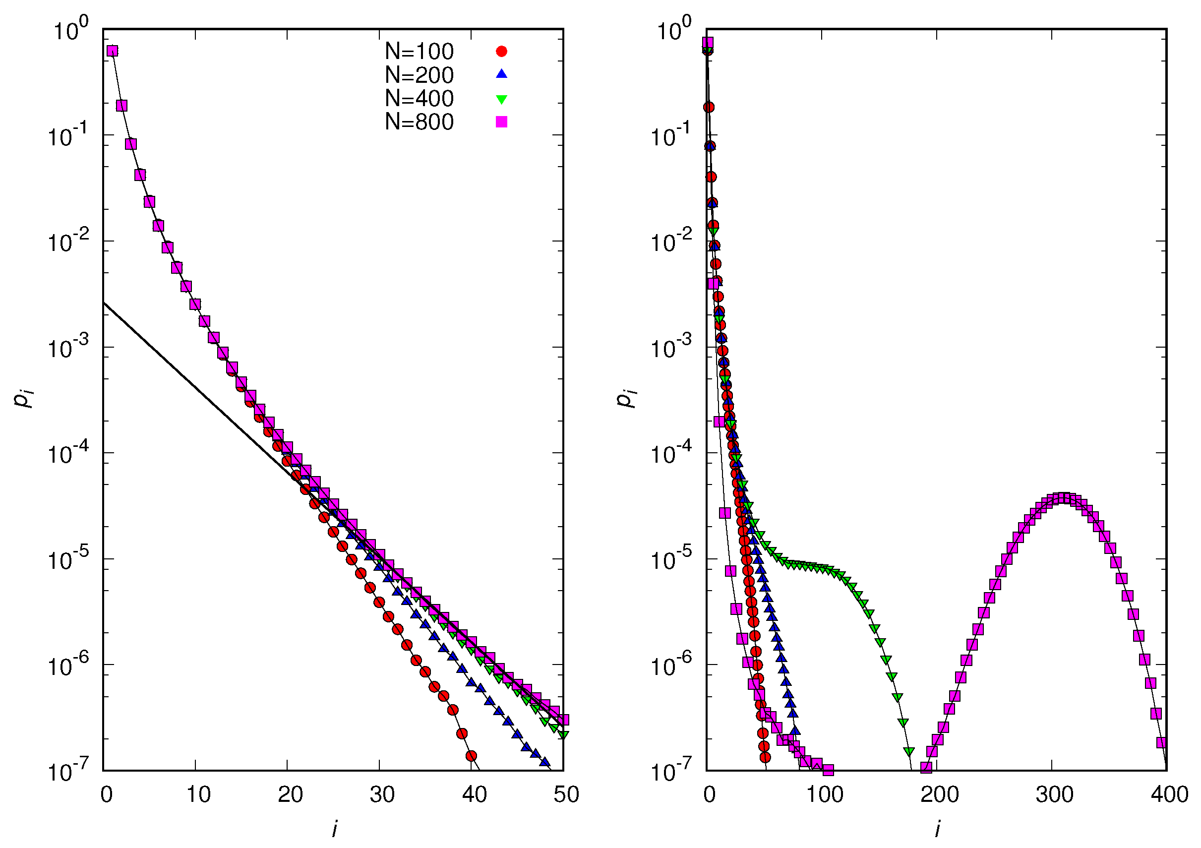
Somewhat disappointingly, the acquisition-and-loss process underlying our model does not produce a power-law decay for the probability of finding large groups. In fact, Figure 10 shows that in the vicinity of the transition point ${\alpha }_c$, where a scale-free behavior is more likely to be observed [27], the probability of observing large groups vanishes exponentially with increasing group size for $\alpha <{\alpha }_c$ or exhibits two peaks for $\alpha >{\alpha }_c$. It remains a challenge to find a simple acquisition-and-loss process that leads to a power-law distribution of group sizes as observed in face-to-face interaction networks [10,11].

6. Discussion

The distribution of sizes is likely the simplest quantitative information we can derive from the observation of freely forming groups. Of course, if the interrelations of the people present were known a priori, we could most certainly predict the formation and composition of some groups. However, here, we follow an alternative and more fruitful approach that ignores any prior knowledge of the individuals present and attempts to explain the observations using stochastic models characterized by a few parameters that represent people’s average tendencies to join and leave a group of a certain size [3,4]. Because the models considered here do not take into account individual idiosyncrasies, we refer to them as null models.

The null models assume that the total number of individuals N is fixed, i.e., that the system is closed, but this assumption is rarely satisfied in field studies of casual groups. For instance, the number of pedestrians on a sidewalk observed on distinct days varies greatly, and it is likely bounded by the city population. However, by taking the limit $N\to \infty$, the fixed-population constraint becomes inconsequential. Of course, when considering this limit, we must focus only on the ratios of the number of groups, as applied in Equation (19). In fact, this was the approach used in the pioneer paper that introduced the mathematical modeling of casual groups [5]. In any event, our results indicate that even for $N=100$, the group-size distribution is practically indistinguishable from the distribution derived in the infinite population limit. Regarding the connection between the field studies and the mathematical models, it is assumed that the acquisition-and-loss process takes place at the time of the formation of the groups and that the system is at equilibrium at the moment of the observation. In addition, it is assumed that the observation happens on a time scale that is much faster than the acquisition-and-loss process, so the groups maintain their sizes during the period of observation [3].

Here, we extend previous models of casual groups by assuming that the appeal of a group of size i to isolates is proportional to $i^{\alpha }$, where $\alpha \in (-\infty ,\infty )$ is the attractiveness exponent. The control of the appeal of groups of different sizes to isolates, which is obtained by tuning the exponent $\alpha$, allows us to consider some interesting scenarios. For instance, large negative values of $\alpha$ could describe people on the sidewalk walking to a dance party, where a predominance of couples is expected, which cannot be explained by the truncated Poisson distribution (see [28] for an alternative, more complex model of couples and isolates). Large positive values of $\alpha$ result in a bimodal distribution of group sizes, corresponding to a scenario where a single large group coexists with a number of isolates. Interestingly, in both cases, the proportion between the number of individuals in the large group or the number of individuals forming couples and the number of isolates is given by the ratio $\kappa$ between the rates of aggregation and disaggregation.

Our main result is that the mean-field approximation used to derive the distribution of group sizes in the case that the attractiveness of a group does not depend on its size (i.e., $\alpha =0$) and in the case that it increases linearly with the group size (i.e., $\alpha =1$) actually yields the exact result for $N\to \infty$. This conclusion, which is drawn from the agreement between the exact stochastic simulations of the group dynamics and the mean-field results, dismisses the suspicion of the inadequacy of the mean-field approximation to describe the equilibrium size distribution of casual groups [6]. (Of course, neither Gillespie’s algorithm [7,8] nor the computational resources to implement it were available in the 1960s to settle this issue.) In fact, for $\alpha \le 1$, the mean-field approximation yields very good predictions, even for a relatively small population size (e.g., $N=100$). However, the approximation fails spectacularly for $\alpha >1$, since it violates the fixed-population constraint. In this case, Gillespie’s stochastic simulation algorithm emerges as the only resource to study the dynamics of casual groups.

In addition, we find that the variation in the attractiveness exponent $\alpha$ produces scenarios where the group sizes are typically small, which is the situation addressed in the literature on casual groups [2], and scenarios where most of the population is confined to a single group. The latter scenario corresponds to the large and stable groups formed by gregarious animals, whose sizes are determined by a variety of selective pressures, such as defense against predation and foraging success [29]; the cognitive load that constrains the number of individuals with whom it is possible to maintain stable relationships [30]; competence in problem solving [31]; and individual distance preservation [32]. Remarkably, in our model, these distinct scenarios are separated by a discontinuous phase transition that takes place at $\alpha ={\alpha }_c>1$, indicating that both types of aggregation behavior can be explained by the same underlying acquisition-and-loss process.

The biological and sociological implication of the success of the null models to produce the empirical distribution of sizes for small groups (i.e., the truncated Poisson distribution) is that prior knowledge of the individuals present in the gathering, as well as individual idiosyncrasies, is not necessary to explain the size distribution of casual groups.

There are at least two research avenues to pursue in order to further improve our understanding of the fleeting clusters of people observed in public gatherings. First, different forms of group attractiveness to isolates can be explored so as to fit the data available from the SocioPatterns collaboration [24], which suggests that the group-size distribution decays as a power law for large group sizes [9,10,11]. Second, the individual-based model that reproduces the SocioPatterns collaboration data [10,11] can be used to fit the small groups’ data available in the seminal works on casual groups [2,3]. If any of these pursuits is successful, one would be able to reproduce all available data on casual groups with a single model.