ConvGRU-RMWP: A Regional Multi-Step Model for Wave Height Prediction

Abstract

Accurate large-scale regional wave height prediction is important for the safety of ocean sailing. A regional multi-step wave height prediction model (ConvGRU-RMWP) based on ConvGRU is designed for the two problems of difficult spatial feature resolution and low accuracy of multi-step prediction in ocean navigation wave height prediction. For multi-step prediction, a multi-input multi-output prediction strategy is used, and wave direction and wave period are used as exogenous variables, which are combined with historical wave height data to expand the sample space. For spatial features, a convolutional gated recurrent neural network with an Encoder-Forecaster structure is used to extract and resolve multi-level spatial information. In contrast to time series forecasting methods that consider only backward and forward dependencies in the time dimension and a single assessment of the properties of the predictor variables themselves, this paper additionally considers spatial correlations and implied correlations among the meteorological variables. This model uses the wave height information of the past 24 h to predict the wave height information for the next 12 h. The prediction results in both space and time show that the model can effectively extract spatial and temporal correlations and obtain good multi-step wave height prediction results. The proposed method has a lower prediction error than the other five prediction methods and verifies the applicability of this model for three selected sea areas along the global crude oil transportation route, all of which have a lower prediction error.

1. Introduction

The influence of the external environment on the ship in the sea voyage comes from two aspects, which are the hydrological environment of the ocean and the meteorological environment of the atmosphere. The elements that have a direct influence on the ship include wind, waves, current, fog, ice, and tide [1]. The wind mainly affects the drift and deflection of the ship, and the waves formed by wind drive will affect the safety and navigation efficiency of the ship [2]. Along with the progress of science and technology, communication between countries is more and more frequent. Shipping is an important means of communication and trade in the world, and sea navigation is tested by waves all the time [3]. The irregularity of sea waves poses a great challenge to maritime navigation safety, maritime scientific research, maritime operations, and the exploitation of ocean energy [4,5]. Therefore, high-precision wave height prediction is helpful in understanding the wave conditions in advance, helping offshore workers plan ahead, maintain the safety of marine navigation, and guarantee smooth and safe marine transportation and offshore operations.

Wave height prediction provides services for ship meteorological and hydrological protection. It takes time for a ship to reach the target area, and multi-step wave height prediction data within a few hours are needed, which are short-term predictions [6]. The wave height prediction data are a time series data of the whole sea area rather than a time series data of a single location. Therefore, the wave height prediction problem is a multi-step spatio-temporal prediction problem.

Numerical wave forecasting methods aim to derive wave characteristics, such as height and period, by solving the wave spectral equations that describe physical processes occurring in the ocean [7]. The mainstream approach for regional wave height prediction is based on numerical models that simulate the physical processes of wave generation and dissipation. The third-generation wave model SWAN [8,9,10] have been developed to accurately simulate wave generation, propagation, and dissipation at various scales, from shallow water to deep water, and has been widely applied in wave simulation [11] and wave energy prediction [12,13]. However, these models require significant computational resources and time to solve the equilibrium equations of wave action, which limits their efficiency and accuracy in long-term simulations of large-scale seas. Therefore, there is a need to balance computational efficiency and simulation accuracy in the development of these models.

Statistical forecasting methods are based on mathematical and statistical approaches that build models to find the relationship between input and output variables based on a large amount of data. Statistical forecasting methods include time series forecasting methods based on traditional parametric models [14,15], time series forecasting methods based on traditional machine learning [16,17,18], and time series forecasting methods based on deep learning [19,20,21]. Among them, the traditional parametric model-based prediction methods are difficult to capture the nonlinear features in the data, and the traditional machine learning-based spatio-temporal sequence prediction methods can automatically capture the nonlinear features in the data and have good generalization ability on small samples. The deep learning-based spatio-temporal sequence prediction methods not only can effectively mine the effective information in the data and automatically capture the hidden linear and nonlinear features but also can efficiently handle large-scale spatio-temporal sequence data [22].

Deep learning algorithms achieve high prediction accuracy by using simple neurons to create nonlinear mapping relations. These models provide explicit solutions and can balance computational efficiency with prediction accuracy, making them suitable for the fast and accurate prediction of large-scale waves [23]. In related work, James et al. [24] proposed a multilayer perceptron (MLP) model for predicting regionally significant wave heights and a support vector machine (SVM) model for identifying regional feature cycles. Machine learning models were developed as accurate and computationally efficient alternatives to the SWAN model, and the alternative models showed strong accuracy in predicting regionally significant wave heights and identifying feature periods in the computational domain. However, wave prediction depends not only on the input at the current point in time but also on the output at previous points in time. This requires machine learning methods that can recognize patterns in time-series data, such as recurrent neural networks or long and short-term memory. Feng et al. [25] developed an MLP model to predict significant wave heights and crystal periods in Lake Michigan. The model considers topographic factors, such as winter icing, and achieves high prediction accuracy with much less computational time than the SWAN model. However, many existing regional wave prediction models rely on MLP models to convert regional wave information into vectors for prediction, which can result in a loss of spatial information and reduced prediction accuracy. Gao et al. [18] developed an LSTM-based model for predicting wave heights at the Bohai Sea hydrographic station. Their results showed that the LSTM model outperformed other models, such as feedforward neural network (FNN) and support vector regression (SVR). Pirhooshyaran and Snyder [26] combined LSTM networks with Bayesian hyperparametric optimization and elastic network methods to develop a sequence-to-sequence neural network for wave height prediction. This novel approach achieved superior results compared to other neural network models in validation. Jing et al. [27] proposed a convolutional neural network(CNN)-based regional wave prediction (CNN-RWP) model using a CNN to construct a mapping relationship between wind data and wave data. The CNN-RWP model and SWAN were compared using a dataset from the Gulf of Mexico. The CNN-RWP model was compared with the SWAN model using a dataset from the Gulf of Mexico, and the average absolute error of both the CNN-RWP model and the SWAN output was less than 10%, but the computational efficiency was improved by a factor of about 1000.

Considering the needs of oceanic navigation, regional wave height prediction for the ocean is of equal importance as wave height prediction for a single significant location. It is important to note that regional wave height prediction does not refer only to multi-location wave height input but rather uses both multiple neighboring location inputs and achieves simultaneous prediction of multiple locations. Regional wave height prediction presupposes that multiple locations with predictions are spatially correlated and, at the same time, temporally correlated between multiple consecutive moments, so this multi-step prediction of regional wave heights is a spatio-temporal prediction problem.

The core of regional wave height prediction is to learn spatial correlation and temporal correlation from a large amount of data, so current spatio-temporal prediction models are mainly based on CNN and RNN. Regional wave height prediction still has the following difficulties.

(1)

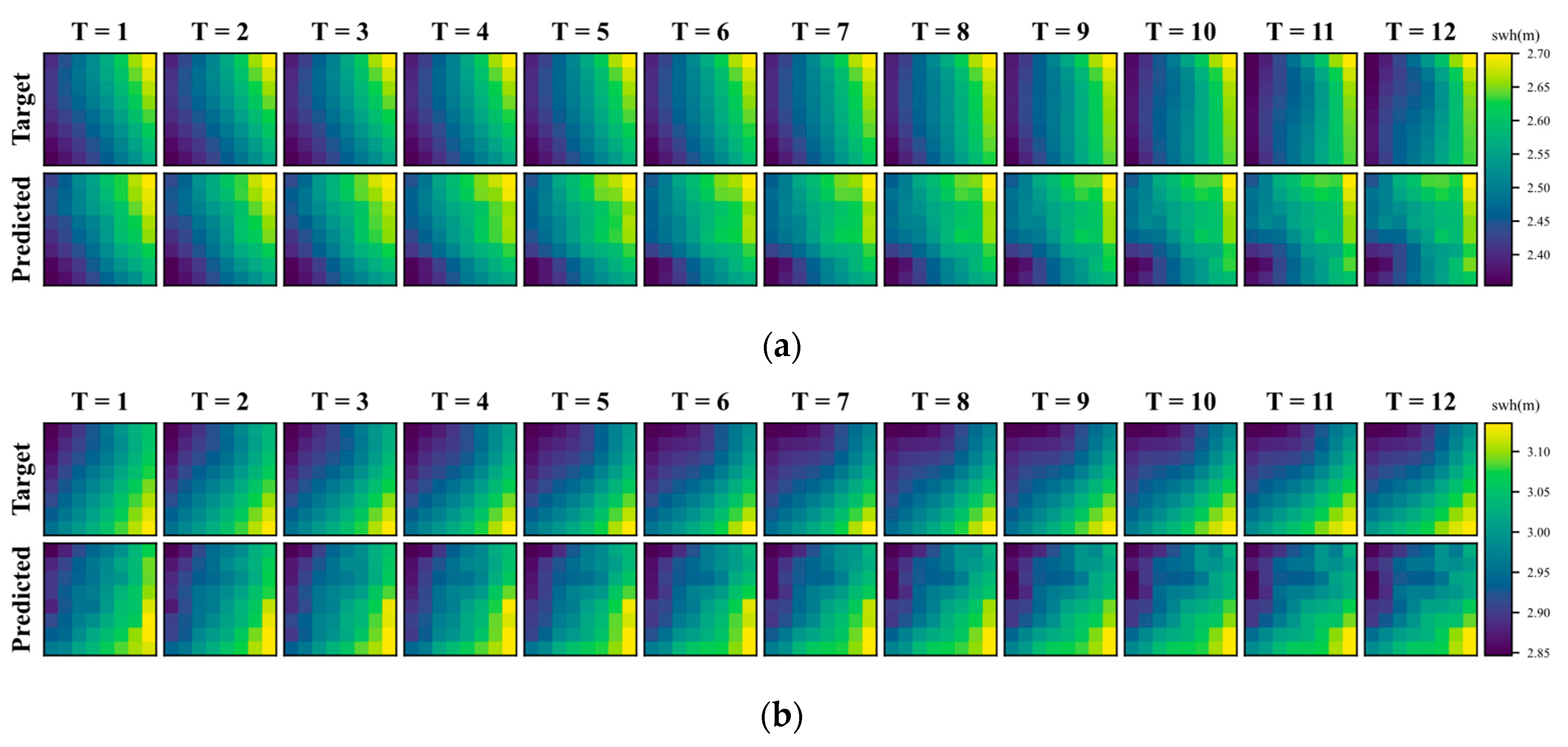
The model needs to output the predicted values of multiple locations simultaneously, which is a pixel-level prediction. Achieving accurate pixel-level spatial output not only requires the model to have strong spatio-temporal feature extraction capabilities but also needs to be able to correctly resolve the extracted deep spatial features to the output map of the same size. For the regional wave height prediction task, direct prediction from the image representation is not suitable, but the deep features should be decoded using the same network layers with gradually increasing output resolution [28]. Thus, regional wave height prediction places high demands on the model structure.

(2)

Performing multi-step prediction while guaranteeing pixel-level regional wave height output is a challenging task. Current regional wave height prediction models, especially CNN-like models, generally perform single-step prediction. Some studies also exist that use independent modeling of individual moments to achieve multi-step prediction, and this approach has difficulty in maintaining high-accuracy prediction at the more backward moments [29].

In recent years, spatio-temporal sequence learning has received more attention than time-series learning because spatio-temporal learning can effectively represent complex spatio-temporal phenomena. Shi et al. [30] proposed a convolutional LSTM (ConvLSTM) network, which combined a convolutional neural network with a recurrent neural network and proved to be able to predict rainfall well from radar images. One advantage of ConvLSTM over CNN is that the former can capture the correlation between time and space. However, ConvLSTM has too many parameters and can easily overwhelm the data [19,20].

In order to address the above problems, this paper combines convolutional neural networks and recurrent neural networks to propose a multi-step spatio-temporal prediction model for wave height based on ConvGRU and using a multi-input multi-output multi-step prediction strategy [31]. The model relies on the encoder-predictor architecture of ConvGRU to construct a mapping of the high-resolution input matrix to the same-resolution output matrix to obtain accurate multi-location prediction results.

The rest of the paper is organized as follows; in Section 2, we present the data and the multi-step spatio-temporal prediction method used in this study. In Section 3, we describe in detail the proposed ConvGRU-based multi-step wave height prediction model for the encoder-predictor region. Section 4 evaluates and discusses the model through experiments. In Section 5, we summarize the conclusions.

2. Data and Methods

2.1. Experimental Data Sources

The data used in this experiment are from the European Reanalysis Dataset Version 5 (ERA5) published by the European Centre for Medium-Range Weather Forecasts (ECMWF), which is freely available on the ECMWF website (https://cds.climate.copernicus.eu/cdsapp#!/dataset/reanalysis-era5-single-levels?tab=form (accessed on 10 August 2022)). ERA5 has provided hourly global atmospheric reanalysis data since 1950, and the experiment selects wave height data “Significant height of combined wind waves and swell (swh),” wave direction data “Mean wave direction (mwd),” and wave period data “Mean wave period (mwp).” swh represents the average height of the highest third of surface ocean/sea waves generated by wind and swell, and it is expressed in meters (m). mwd is the mean direction of waves in the first swell partition, and it is expressed in degrees (°). Mwp is the average time it takes for two consecutive wave crests on the surface of the ocean/sea to pass through a fixed point, and it is measured in seconds (s). In order to confirm the effect of the protection of ocean shipping, a rectangular sea area is selected on the main transportation route of the world crude oil trade, as shown in Figure 1, which is located in the Arabian Sea, the Arabian Sea is located between the Horn of Africa and the south of Asia, part of the Indian Ocean, and is a major transportation route worldwide [32]. Tropical cyclones often occur in summer and autumn, accompanied by strong winds and heavy rainfall [33,34]. The grid size of the selected area is 8 × 8, and the coordinates of the upper left corner are (15 N, 60 E). The spatial and temporal series of the sea area during 2020–2021 is extracted from ERA5, which contains 17,544 h of data. The maximum value of wave height in this area is 5.9778 m, the minimum value is 0.9877 m, the mean value is 2.2551 m, the variance is 0.4121 m², and the standard deviation is 0.6420 m.

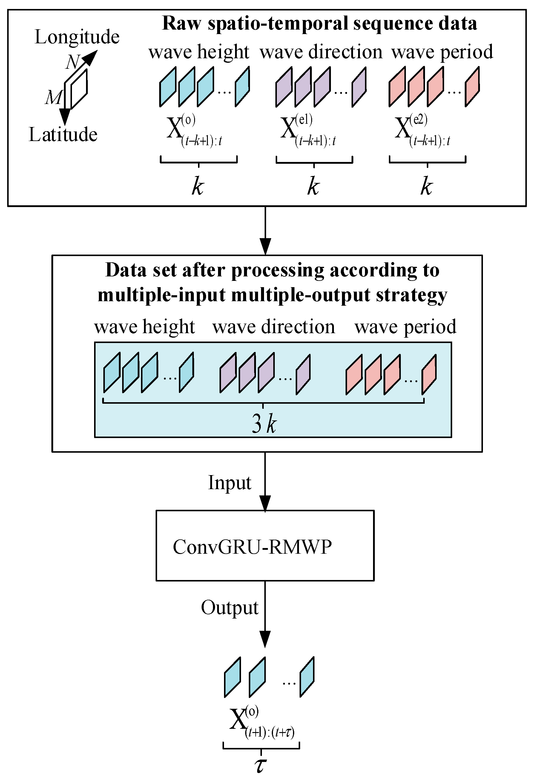
2.2. Multi-Input Multi-Output Strategy (MIMO)

The prediction problem of regional wave height is treated as a spatio-temporal sequence-to-temporal sequence regression problem. Spatiotemporal sequences can be considered as single-channel pictures at each moment, so the deep CNN-based model is well suited to handle such problems. By using the input time step as the input channel, the convolutional layer can extract features from the spatio-temporal data. In order to achieve multi-step prediction, spatio-temporal sequence prediction can be made using the Direct Multi-step strategy (DMS). DMS models the data separately for each moment to be predicted, and H-step prediction requires building H-independent models. These models use the same input data to predict variables at different moments and determine the parameters of each model by minimizing the prediction error at the corresponding moment. Currently, most CNN-based wave height prediction models use DMS, a strategy that requires the CNN model to output a single channel image as a single-step prediction and to build independent prediction models with the same structure for each output moment, with the results of all independent prediction models collectively serving as multi-step prediction values. This strategy requires very large computational resources and is not suitable for tasks with higher prediction time resolution and longer prediction time steps. At the same time, because each prediction moment is independent of the other and the historical moment only has a high correlation with the wave height at the approaching moment, this strategy can obtain better prediction results at the approaching moment, but the prediction results will deteriorate at the backward moment [30]. Since it takes some time to reach the edge of the region during the ship navigation, the regional wave height prediction requires higher prediction accuracy at the leeward moment, and DMS cannot meet the requirements well. MIMO uses a single model to obtain multiple prediction values by a single calculation, and its prediction formula is shown in Equation (1). MIMO is suitable for models that support multivariate inputs and multivariate outputs, such as vector autoregression and various types of neural networks. MIMO has the advantages of relatively small computational resources and no cumulative error and is the most suitable multi-step prediction strategy for neural networks.

$${\widehat{x}}_{(t+1):(t+H)}=f(x_{(t-L+1):t};\mathsf{\theta })$$

(1)

where $x_{(t-L+1):t}=\{x_{t-L+1},x_{t-L+2},\dots ,x_t\}\in {ℝ}^L$ is the true value of the variable at the previous $L$ moments and ${\widehat{x}}_{(t+1):(t+H)}=\{{\widehat{x}}_{t+1},{\widehat{x}}_{t+2},\dots ,{\widehat{x}}_{t+H}\}\in {ℝ}^H$ is the predicted value of the variable at the subsequent $H$ moments. The variable $f$ represents the mathematical model based on the true values of the historical variables and the variable to be predicted and $\mathsf{\theta }$ represents the model parameters. In this paper, the multi-step prediction of the wave height region uses the MIMO strategy, under which the model uses $H$ output channels to perform $H$-step prediction, and the total prediction result is a three-dimensional matrix of dimension A.

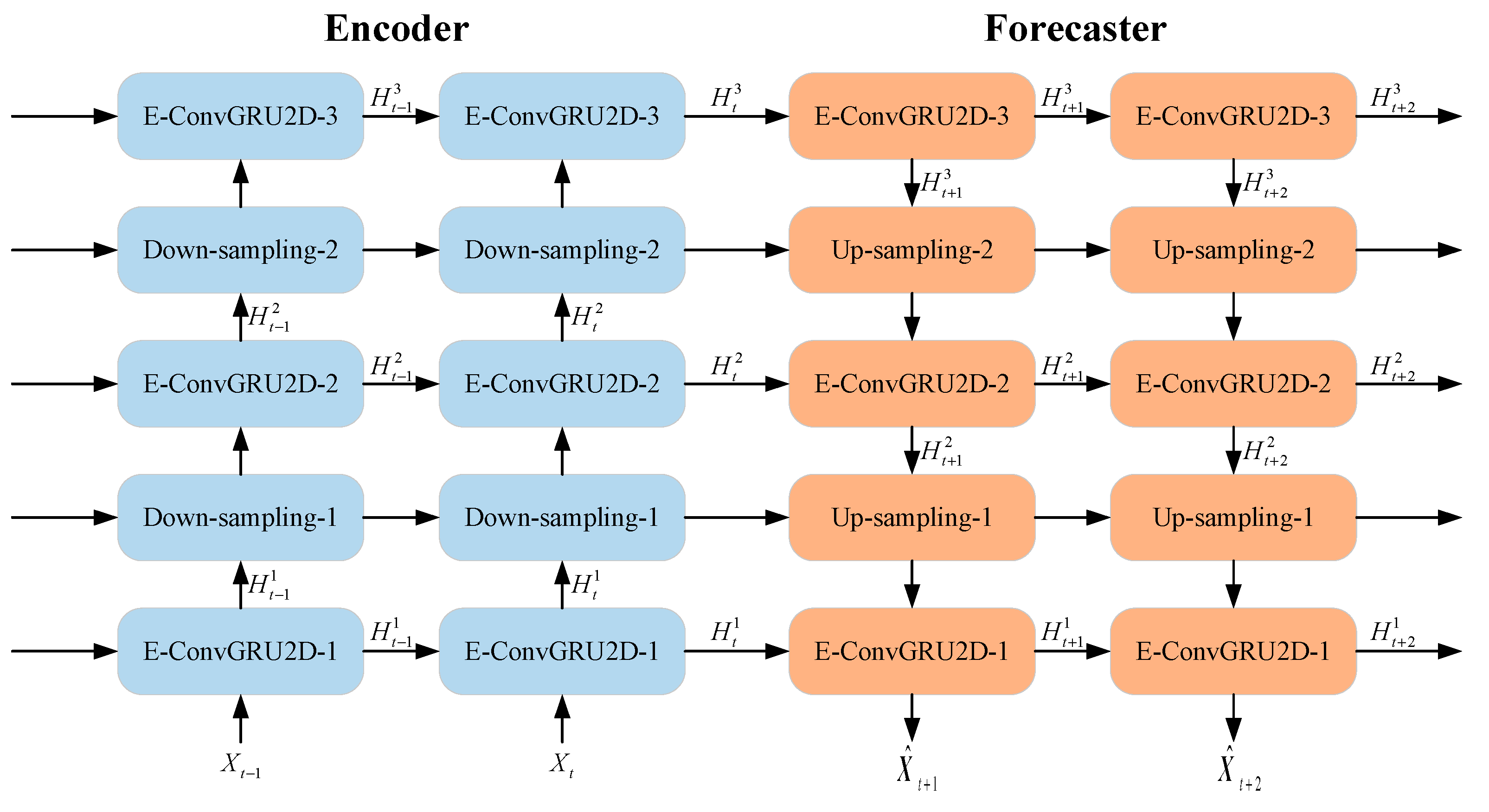
2.3. Multi-Step Spatio-Temporal Prediction Method

Wave height information for multiple locations over a long period of time is required for ocean-going vessels. The traditional single-location wave height prediction can hardly meet the information demand on a large scale. Therefore, the multi-location wave height multi-step prediction problem is defined as a spatio-temporal multi-step prediction problem. The wave height data of a sea area are suitable to be represented by a matrix, which belongs to a regular grid form. The prediction of regional wave heights requires simultaneous input and prediction of wave height values at multiple locations and is, therefore, a multi-step spatio-temporal prediction problem on a regular grid. An origin point with coordinates $(0,0)$ is specified on the map, and for $\mathrm{M}\times \mathrm{N}$ locations with this point as the upper left corner, a regular grid region is formed. The wave height prediction problem in this grid region can be expressed in the following form.

The $\mathrm{M}\times \mathrm{N}$ rectangular grid represents the prediction area, where the coordinates of each sea location are $(\mathrm{i},\mathrm{j})$. At the time $t$, $x_t(\mathrm{i},\mathrm{j})$ represents the observed value of the variable at the location $(\mathrm{i},\mathrm{j})$.

$${\mathrm{x}}_t=\left[\begin{array}{ccc}{x}_t(1,1)& \cdots & x_t(1,N)\\ ⋮& \ddots & ⋮\\ x_t(M,1)& \cdots & x_t(M,N)\end{array}\right]\in {ℝ}^{M\times N}$$

(2)

${\mathrm{X}}_{1:k}=\{{\mathrm{x}}_1,{\mathrm{x}}_2,\dots ,{\mathrm{x}}_k\}\in {ℝ}^{\mathrm{M}\times \mathrm{N}\times k}$ denotes a temporal sequence of variable matrices at $k$ moments in time order. In the univariate multi-step momentary prediction problem, the variable matrix at $\tau$ future moments is predicted using the known variable matrix at $k$ past moments.

$${\hat{\mathrm{X}}}_{(t+1):(t+\tau )}^{}=f({\mathrm{X}}_{(t-k+1):t}^{};\mathsf{\theta })$$

(3)

where $f$ is a function of the prediction model and $\mathsf{\theta }$ is a matrix composed of the model parameters.

In a practical forecasting task, to improve the accuracy of time series forecasting, it is not usual to model only the variable to be predicted with its historical data. In some cases, the error of the model can be further reduced by adding exogenous variables to the input data that are highly correlated with the variable to be predicted. The introduction of exogenous variables provides effective information for the prediction of the target variable. Letting the target variable be $o$, and the single exogenous variable be $e$, the multi-step time-series prediction can be represented by Equation (4). In this paper, the target variable is wave height, and the exogenous variables are wave direction and wave period. The schematic diagram of multi-step time series prediction based on ConvGRU-RMWP is shown in Figure 2.

$${\hat{\mathrm{X}}}_{(t+1):(t+\tau )}^{(\mathrm{o})}=f({\mathrm{X}}_{(t-k+1):t}^{(\mathrm{o})},{\mathrm{X}}_{(t-k+1):t}^{(\mathrm{e})};\mathsf{\theta })$$

(4)

3. Model Building and Experimental Setup

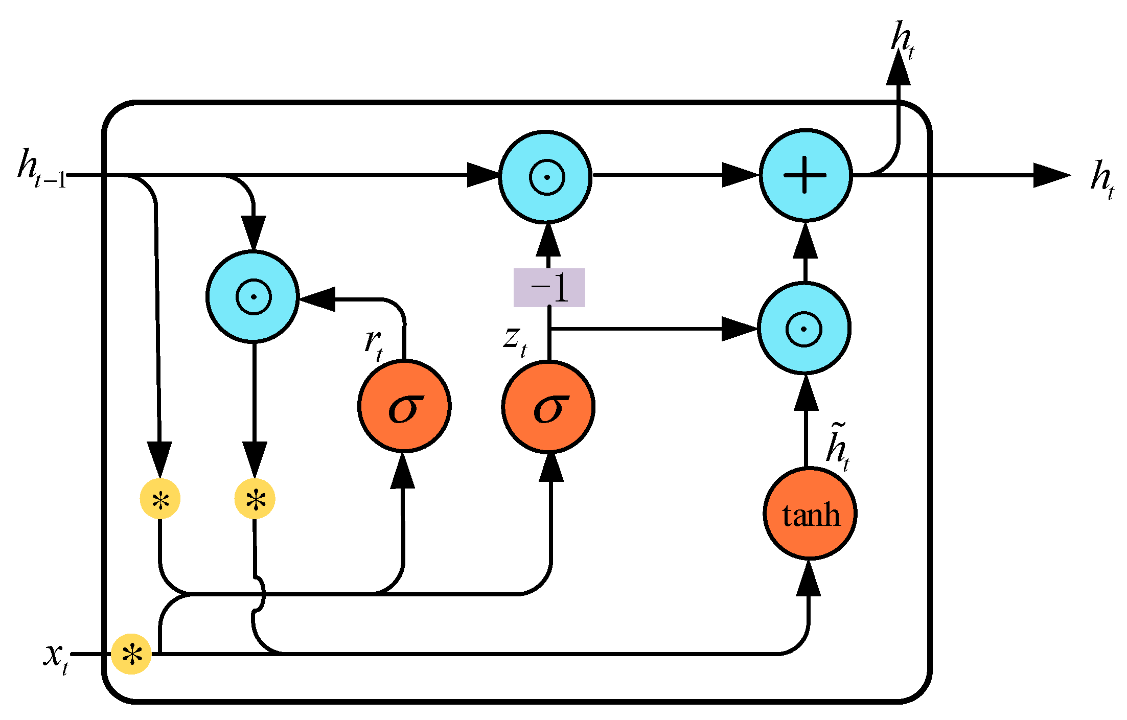
3.1. ConvGRU Network

Because the traditional recurrent neural network (RNN) cannot handle long-term dependence well due to the exploding gradient or vanishing gradient generated during training, the Gated Recurrent unit (GRU) is an improvement on the traditional recurrent neural network RNN, which is a variant of the Long Short-Term Memory Neural Network LSTM, simplifying the structure of the LSTM with only an update gate and a reset gate [35]. The GRU model has fewer parameters and is a simpler model but maintains the same performance as the LSTM with faster training convergence time. It inherits the ability of RNN to explore the intrinsic dependencies of sequence data but also solves the problems of vanishing gradient, long training time, and overfitting caused by the long sequences of traditional RNN and improves the local optimization ability and network generalization ability [36,37]. Compared with GRU networks, convolution-based gated recurrent unit (ConvGRU) neural networks have stronger learning ability, so this paper uses convolution-based GRU (ConvGRU) for modeling, and the ConvGRU structure cannot only establish temporal relationships, such as GRU, but also carve out local spatial features, such as CNN. The internal structure of ordinary LSTM and GRU adopts a nearly fully connected approach, which brings serious information redundancy problems, and this connection ignores the spatial correlation between local pixels in the data. ConvGRU extends the idea of being fully connected in GRU to the convolutional structure and replaces the dot product operation in GRU with the convolution operation, and the internal structure of ConvGRU is shown in Figure 3. A feature and advantage of this design is that all the input and output elements are three-dimensional tensors, which preserve spatial information.

With the memory feature in GRU, ConvGRU can preserve the features of historical input image sequences during training, which can also ensure the effective transfer of feature information over a longer period and improve the accuracy of prediction results, calculated as follows.

$$z_t=\sigma \left(W_{xz}\ast x_t+W_{hz}\ast h_{t-1}+b_z\right)$$

(5)

$$r_t=\sigma \left(W_{xr}\ast x_t+W_{hr}\ast h_{t-1}+b_r\right)$$

(6)

$${\tilde{h}}_t=\tanh \left(W_{xh}\ast x_t+W_{hh}\ast \left(r_t\odot h_{t-1}\right)+b_h\right)$$

(7)

$$h_t=z_t\odot {\tilde{h}}_t+\left(1-Z_t\right)\odot h_{t-1}$$

(8)

$r_t$ is the reset gate, $z_t$ is the update gate, ${\tilde{h}}_t$ is the current memory information, and $h_t$ is the final memory information. $x_t$ is the information input at the current moment, $h_{t-1}$ is the hidden layer output at the previous moment, and $b_i$ and $W_{ij}$ are the respective bias and weight matrices. The symbol “$\ast$” denotes the convolution operator, “$\odot$” denotes the Hadamard product, and “$\sigma$” denotes the Sigmoid function. The structure selects the information through a gate structure composed of Sigmoid layers and convolutional operations. Whenever a new input arrives, the reset gate controls the decision to clear the previous state, and the update gate controls the amount of new information entering the state.

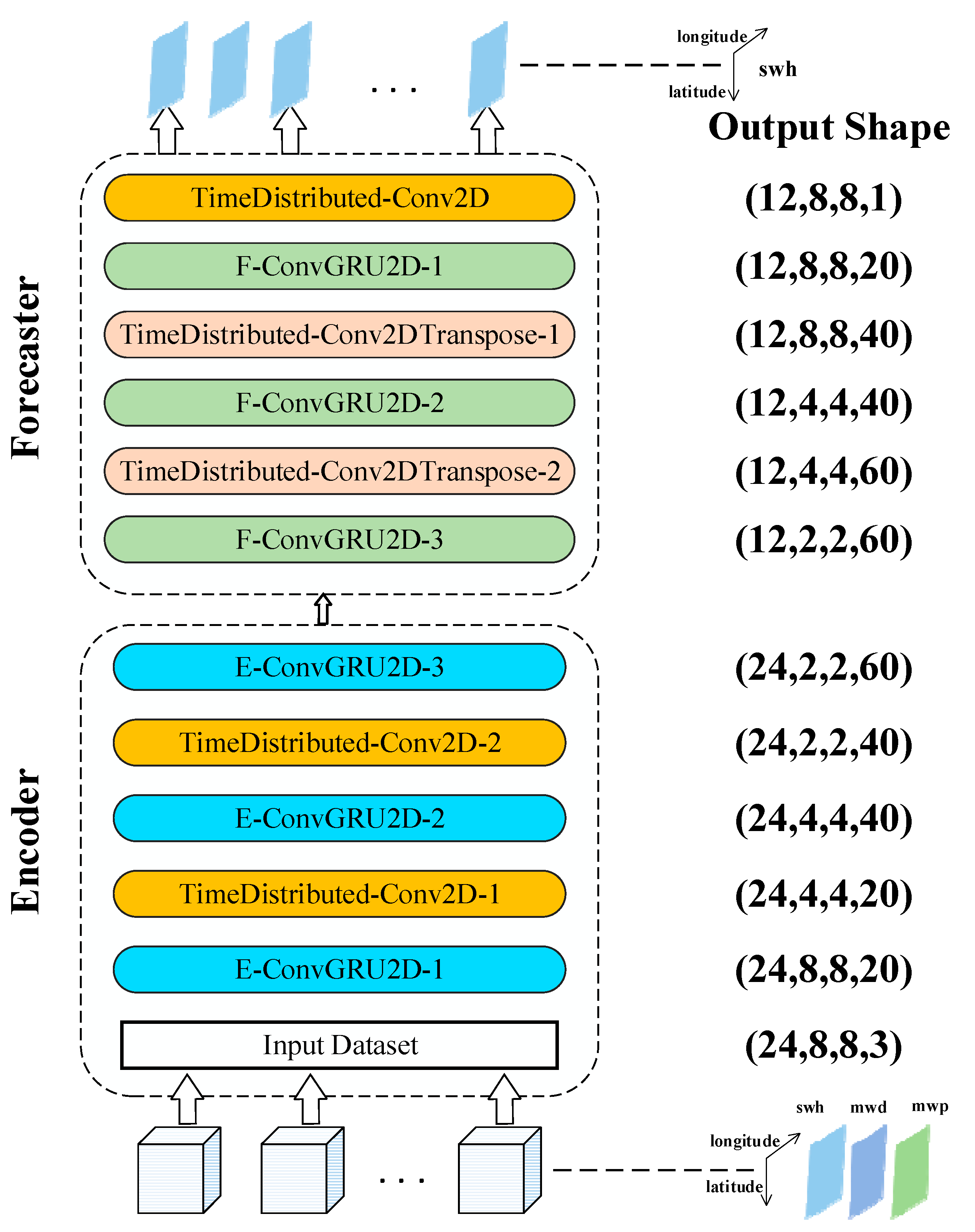
3.2. Model Building

To ensure that the model can represent spatio-temporal features well and effectively predict changes in wave height spatio-temporal sequences, an encoder-predictor structure similar to that of Shi et al. [30] is used to predict spatio-temporal sequences. The encoder module consists of two convolutional downsampling layers and three ConvGRU layers. The predictor module consists of two transposed convolutional upsampling layers and three ConvGRU layers.

Using the wave height values and wave height directions of the past 24 h, a three-layer Encoder-Forecaster model is built based on the ConvGRU framework for training to establish a spatio-temporal prediction model for wave height values and to predict the wave height values for the next 12 h. Figure 4 shows the network structure of the Encoder-Forecaster model. The Encoder module learns the image features from low-dimensional to high-dimensional, i.e., after the convolutional downsampling to reduce the image feature size and the ConvGRU unit to learn the image sequence features, the intermediate vector is obtained, and then the intermediate vector is input to the Forecaster forecasting module, and the transposed convolutional upsampling part of the Forecaster module increases the image feature size and the ConvGRU unit learns the image sequence features, and output the future region wave height values. The loss function is continuously updated during the training process so that the loss function value is continuously reduced.

Figure 5 shows the change of the feature map during the process of the model from the Encoder module to the Forecaster module. In the Encoder phase, the size of the feature map gradually becomes smaller while the number of channels gradually increases, and the extracted features gradually change from low-dimensional to high-dimensional, and in the Forecaster phase, the size of the feature map gradually becomes larger while the number of channels gradually becomes smaller, until finally the output image with the same size as the input image is obtained.

3.3. Loss Function and Model Setup

The regional wave height prediction model uses the Frobenius paradigm as the loss function and performs one gradient calculation and network parameter update using the loss function value of each batch. Compared with using the entire sample set for a single parameter update, this strategy improves the computational speed and facilitates the search for extreme value points on large data sets. The loss function on each batch is shown in Equation (9).

$$J=\frac{1}{M\times N\times C}{\displaystyle \sum _{c=1}^C{\Vert {\mathrm{x}}^{(\mathrm{o})}-{\hat{\mathrm{x}}}^{(\mathrm{o})}\Vert }_F^2}$$

(9)

where $C$ denotes the number of samples in this batch, and the size is equal to the batch size. The variable $C$ is an integer multiple of $\tau$ to ensure that a set of $\tau$-step prediction samples appear in the same batch. The variables ${\mathrm{x}}^{(\mathrm{o})}$ and ${\hat{\mathrm{x}}}^{(\mathrm{o})}$ represent the true and predicted values of the target variable (wave height) corresponding to the samples, respectively, both containing $M\times N$ elements.

The hyperparameters of the model are batch size set to 12 and learning rate set to 0.001, and the model uses Adam optimizer. (The parameter settings are explained in Section 4.1) The training process uses an Encoder-Forecaster network consisting of three layers of ConvGRU, and the information on the network structure parameters is shown in

Table 1. ConvGRU network structure parameter information.

Parts	Network Layer	Filters	Kernel_Size	Strides
Input	Input-1
Encoder	E-ConvGRU2D-1	20	2	1
	TimeDistributed-Conv2D-1	20	2	2
	E-ConvGRU2D-2	40	2	1
	TimeDistributed-Conv2D-2	40	2	2
	E-ConvGRU2D-3	60	2	1
Forecaster	F-ConvGRU2D-3	60	2	1
	TimeDistributed-Conv2DTranspose-2	60	3	1
	F-ConvGRU2D-2	40	2	1
	TimeDistributed-Conv2DTranspose-1	40	2	2
	F-ConvGRU2D-1	20	2	1
output	TimeDistributed-Conv2D	1	1	1

. The multi-layer ConvGRU can be used to obtain information on the wave height data in both temporal and spatial dimensions to better establish temporal relationships. Dropout allows each iteration to go randomly to update the network parameters. Introducing such randomness not only increases the ability to handle wave height data but also keeps the input and output neurons unchanged by randomly deleting some hidden neurons in the network layers and back propagating the errors through the modified network by the operation of forward propagation.

3.4. Experimental Setup and Evaluation Indicators

The hardware platform is equipped with NVIDIA GeForce RTX 3080, GPU configuration CUDA 11.3 parallel framework, and cuDNN8.2 acceleration library. The model is built based on Tensorflow 2.3.0 and Numpy 1.18.5, and the code is based on Python 3.8.

The first 24 h of data were used in the experiment to predict the second 12 h. The data set samples were divided into training, validation, and test sets in a 4:1:1 ratio. Standard wave height, mean wave direction, and mean wave period were subjected to [–1, 1] maximum-minimum normalization, and inverse normalization was performed before evaluating the prediction results. The models are trained using the training set, hyperparameterized using the validation set, and the prediction results are derived using the test set. The weight matrices and bias vectors of all deep learning models are initialized using normal distributions. All deep learning models are trained using batches, and the maximum training period (epochs) for the ConvGRU-based models is 30, and the optimizer is Adam.

Evaluation metrics and images are used to evaluate the prediction results. Both evaluation metrics and comparison images are used to accurately quantify the strengths and weaknesses of different models’ prediction results while enabling visual comparisons from different perspectives. In order to evaluate the results of a single prediction moment in multi-step forecasting, the average results of all locations in a single prediction moment in regional multi-step forecasting are evaluated using root mean square error ${\mathrm{RMSE}}_t$, mean absolute error ${\mathrm{MAE}}_t$, and mean absolute error percentage ${\mathrm{MAPE}}_t$, with the three indicators expressed as shown in Equations (10)–(12).

$${\mathrm{RMSE}}_t=\sqrt{\frac{1}{M\times N}{\displaystyle \sum _{\mathrm{i}=1}^M{\displaystyle \sum _{\mathrm{j}=1}^N{(x_{i,j,t}-{\widehat{x}}_{i,j,t})}^2}}}$$

(10)

$${\mathrm{MAE}}_t=\frac{1}{M\times N}{\displaystyle \sum _{\mathrm{i}=1}^M{\displaystyle \sum _{\mathrm{j}=1}^N|x_{i,j,t}-{\widehat{x}}_{i,j,t}|}}$$

(11)

$${\mathrm{MAPE}}_t=\frac{1}{M\times N}{\displaystyle \sum _{\mathrm{i}=1}^M{\displaystyle \sum _{\mathrm{j}=1}^N\frac{|x_{i,j,t}-{\widehat{x}}_{i,j,t}|}{\left|x_{i,j,t}\right|}}}\times 100\%$$

(12)

$x_{i,j,t}$ and ${\widehat{x}}_{i,j,t}$ represent the true and predicted values of wave height at the $(i,j)$ coordinate, respectively. The closer the $\mathrm{RMSE}$ and $\mathrm{MAE}$ are to 0, the lower the prediction error in meters. The $\mathrm{MAPE}$ is also closer to 0 the lower the prediction error in %. In order to evaluate the multi-step spatio-temporal prediction effect as a whole, the mean values of the above indicators at $H$ prediction time steps are taken and denoted as $\mathrm{MRMSE}$, $\mathrm{MMAE}$, and $\mathrm{MMAPE}$, respectively.

4. Results and Discussion

4.1. Optimal Setting of Hyperparameters

After determining the use of MRMSE, MMAE, and MMAPE as evaluation metrics, a hyperparameter grid search is performed for the regional wave height multi-step prediction model set up for this experiment. The training hyperparameters include the batch size and the learning rate of the Adam optimizer. The experiments were conducted, and the MRMSE, MMAE, and MMAPE under different hyperparameters were obtained, as shown in

Table 2. MRMSE, MMAE, and MMAPE under different hyperparameters.

Learning Rate	Batch Size	MRMSE	MMAE	MMAPE
0.001	12	0.0986	0.0710	3.1375
	24	0.1003	0.0742	3.3980
	36	0.1005	0.0772	3.7344
	48	0.1086	0.0781	3.4124
0.0001	12	0.1037	0.0751	3.3259
	24	0.1096	0.0796	3.5492
	36	0.1192	0.0912	4.1226
	48	0.1259	0.0924	4.0918

, and the bold entries indicate the best results and the best combination of training hyperparameters under this network setup was: a batch size of 12 and learning rate of 0.001.

4.2. Comparison of Prediction Errors for Different Input Steps

To prove that the input 24 h is the better choice. The comparison experiments with different input steps were performed under the best hyperparameters selected. 12–36 h was chosen as the input, and the results are shown in

Table 3. Prediction error results with different input steps.

Input Step	Error	1	2	3	4	5	6	7	8	9	10	11	12	Mean
12	RMSE	0.0625	0.0621	0.0710	0.0802	0.0905	0.1009	0.1112	0.1211	0.1310	0.1410	0.1513	0.1618	0.1070
	MAE	0.0521	0.0508	0.0580	0.0653	0.0731	0.0810	0.0886	0.0959	0.1032	0.1108	0.1186	0.1268	0.0853
	MAPE	2.6415	2.5395	2.8811	3.1963	3.5357	3.8824	4.2226	4.5467	4.8738	5.2075	5.5558	5.9160	4.0832
18	RMSE	0.0586	0.0613	0.0666	0.0753	0.0846	0.0943	0.1038	0.1131	0.1222	0.1314	0.1409	0.1506	0.1002
	MAE	0.0470	0.0480	0.0508	0.0567	0.0630	0.0699	0.0767	0.0833	0.0898	0.0965	0.1034	0.1105	0.0746
	MAPE	2.2392	2.2435	2.3417	2.5848	2.8528	3.1510	3.4457	3.7356	4.0225	4.3119	4.6123	4.9241	3.3721
24	RMSE	0.0446	0.0499	0.0594	0.0704	0.0819	0.0935	0.1047	0.1155	0.1258	0.1359	0.1459	0.1559	0.0986
	MAE	0.0345	0.0372	0.0428	0.0501	0.0583	0.0667	0.0748	0.0826	0.0902	0.0975	0.1049	0.1122	0.0710
	MAPE	1.6250	1.7045	1.9111	2.2194	2.5661	2.9332	3.2848	3.6306	3.9610	4.2808	4.6043	4.9291	3.1375
30	RMSE	0.0667	0.0702	0.0778	0.0872	0.0976	0.1081	0.1187	0.1292	0.1397	0.1501	0.1607	0.1712	0.1149
	MAE	0.0559	0.0590	0.0646	0.0716	0.0796	0.0874	0.0951	0.1027	0.1103	0.1179	0.1257	0.1337	0.0920
	MAPE	2.8505	2.9459	3.1930	3.5026	3.8721	4.2303	4.5832	4.9276	5.2784	5.6257	5.9892	6.3630	4.4468
36	RMSE	0.0531	0.0573	0.0645	0.0752	0.0859	0.0975	0.1088	0.1200	0.1310	0.1416	0.1522	0.1625	0.1041
	MAE	0.0390	0.0414	0.0463	0.0540	0.0614	0.0698	0.0779	0.0861	0.0942	0.1023	0.1103	0.1183	0.0751
	MAPE	1.8427	1.9254	2.1101	2.4518	2.7490	3.1248	3.4698	3.8315	4.1820	4.5358	4.8873	5.2410	3.3626

, with bold entries indicating the best results.

4.3. Predicted Results

After determining the input steps, to visualize the performance of the proposed model, the prediction results are presented from both spatial and temporal perspectives, considering that the output data are multi-step spatio-temporal prediction results. The results of the spatial perspective are shown in Figure 6, which illustrates the comparison between the target and predicted images of the sample at the 1st, 2nd, …, and 12th hour.

In Figure 6, the regional wave height prediction model obtained better results for both samples. In sample A, the prediction map is very similar to the real map in the t = 1–7 h images. In the t = 7–12 h images, in the edge region, the prediction is better, and in the middle region, the prediction is worse. The wave height in sample B changes faster, and the prediction is more difficult than that in sample A. The prediction map has a delay, but the trend of the wave height values at different locations on each time step is consistent with the true map, and the overall error is still low, which can ensure a highly accurate prediction. The changing trend of wave height in the images in both samples A and B can be better reflected, and better results are obtained in each prediction moment.

The results of the time angles on three randomly selected locations from the A and B samples selected in the test set are shown in Figure 7.

As can be seen in Figure 7, the model’s prediction results are accurate from a time perspective. As shown in (c) and (d), the model outputs the correct “up then down” variation. As shown in subfigures (a) and (e), the model outputs the correct “overall up” variation. Subplots (b) and (f) have opposite trends in some time periods, but the errors are small. This indicates that the prediction model can obtain the correct pattern of changes for most of the time periods for all types of time trends.

4.4. Ablation Experiments

Since wave height (swh), mean wave direction (mwd), and mean wave period (mwp) can jointly express wave phenomena, the regional wave height prediction model uses mwd and mwp as exogenous variables to improve the accuracy of swh prediction. The MIMO strategy has the advantages of relatively small computational resources, no cumulative errors, and small computational resource requirements and is the most suitable multi-step prediction for neural networks strategy. In order to confirm that the above two changes bring enhancements to the model, the following ablation experiments are conducted based on the control variable method.

4.4.1. Impact of Exogenous Variables

The mwd exogenous variable is added considering the need to predict wave heights at multiple proximity locations. Considering the need to predict multi-step wave heights, the mwp exogenous variable is added. To confirm the enhancement of the exogenous variables on the prediction effect, mwd, and mwp are selected as exogenous variables for comparison experiments. The results are shown in

Table 4. MRMSE, MMAE, and MMAPE under different exogenous variables.

Input Variables	MRMSE	MMAE	MMAPE
swh	0.1091	0.0802	3.5561
swh,mwd	0.1075	0.0785	3.4959
swh,mwd,mwp	0.0986	0.0710	3.1375

, and the bold entries indicate the best results.

A major improvement in the regional multi-step wave height prediction is obtained from the wave phenomenon mechanism by correlating wave direction and wave period with wave height and using them as exogenous variables in the interpretable series prediction. As shown in Table 4, the MRMSE, MMAE, and MMAPE of the prediction model are reduced by 1.47%, 2.12%, and 1.69%, respectively, by adding the mean wave direction. The addition of wave direction and wave period variables reduces the MRMSE, MMAE, and MMAPE of the prediction model by 9.62%, 11.47%, and 11.77%, respectively. Therefore, the simultaneous input of wave direction and wave period exogenous variables can effectively assist regional multi-step wave height prediction, reduce the fluctuation of the output, and improve prediction accuracy.

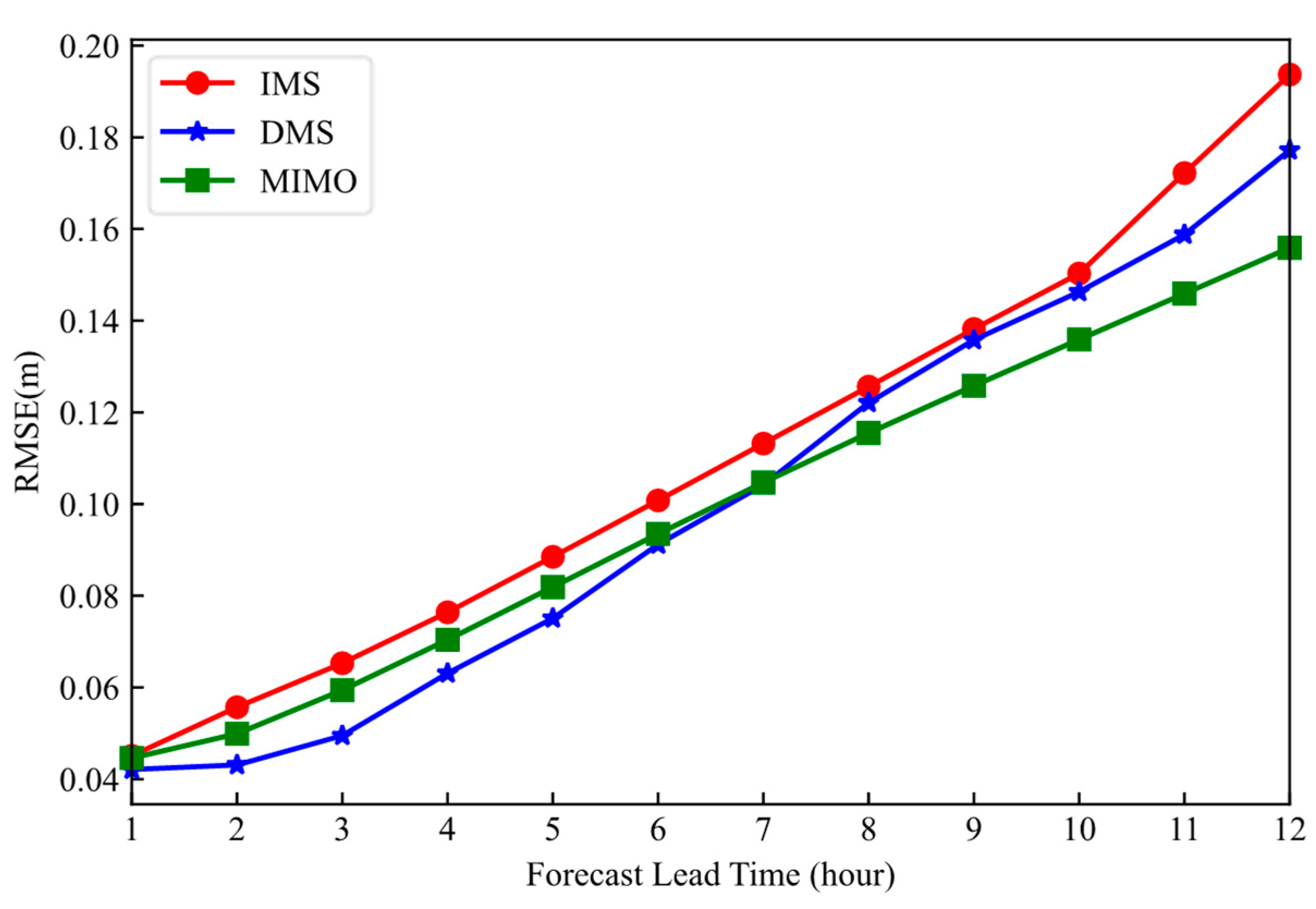
4.4.2. Impact of Multiple Input—Multiple Output Strategy (MIMO)

The prediction effectiveness of the model also depends on the forecasting strategy used. The Iterative Multi-step strategy (IMS) strategy starts with a single-step prediction, after which the single-step prediction is added to the end of the input vector, the first element is removed, and the same model is re-entered for prediction. Each prediction of the IMS still produces a single prediction, and the $H$-step prediction is obtained by iterating $H$ times. The Direct Multi-step strategy (DMS) strategy models the data separately for predicting each moment. Implementing $H$-step prediction requires building $H$ independent models that use the same input data and predict variables at different moments. To confirm the enhancement brought by the MIMO strategy, IMS, DMS, and MIMO are compared. Since the trends of RMSE, MAE, and MAPE error curves are almost the same, only the RMSE error results are shown in Figure 8.

As can be seen from Figure 8, the error of the multi-input multi-output strategy is slightly higher than that of the direct multi-step prediction strategy at the approaching moments from 1–6 h and significantly lower from 8–12 h. The error of the iterative multi-step prediction strategy gradually increases with the increase in the prediction step length, and the errors are all larger than those of the multi-input multi-output strategy. The above results demonstrate that the multi-input multi-output strategy can improve the prediction effect at a later time, and the computational resources of the multi-input multi-output strategy are relatively small compared with the direct multi-step prediction strategy. Compared with the iterative multi-step prediction strategy, the multi-input multi-output strategy has no cumulative error advantage and is the most suitable multi-step prediction strategy for the regional prediction task, which can meet the requirements of the ocean navigation regional wave height prediction for the leaning moment prediction with high accuracy.

4.5. Comparison of Different Models and Prediction Results

The regional multi-step wave height prediction model designed in this paper needs to be compared with various advanced models to confirm its superiority. The SVR, MLP, LSTM, GRU, and CNN+GRU models are selected for comparison. The SVR, MLP, LSTM, and GRU models are designed to predict the time series of a single location for spatio-temporal sequence data, and 64 wave height-wave direction-wave period prediction wave height models are established, and all prediction results are summarized as time series. The CNN+GRU model spatio-temporal Sequence data, designed to predict the spatial sequences of a single moment, built 12 wave height-wave direction-wave period prediction wave height models and aggregated all prediction results into spatial sequences. mwd and mwp exogenous variables were added to SVR, MLP, LSTM, GRU, and CNN+GRU models.

(1)

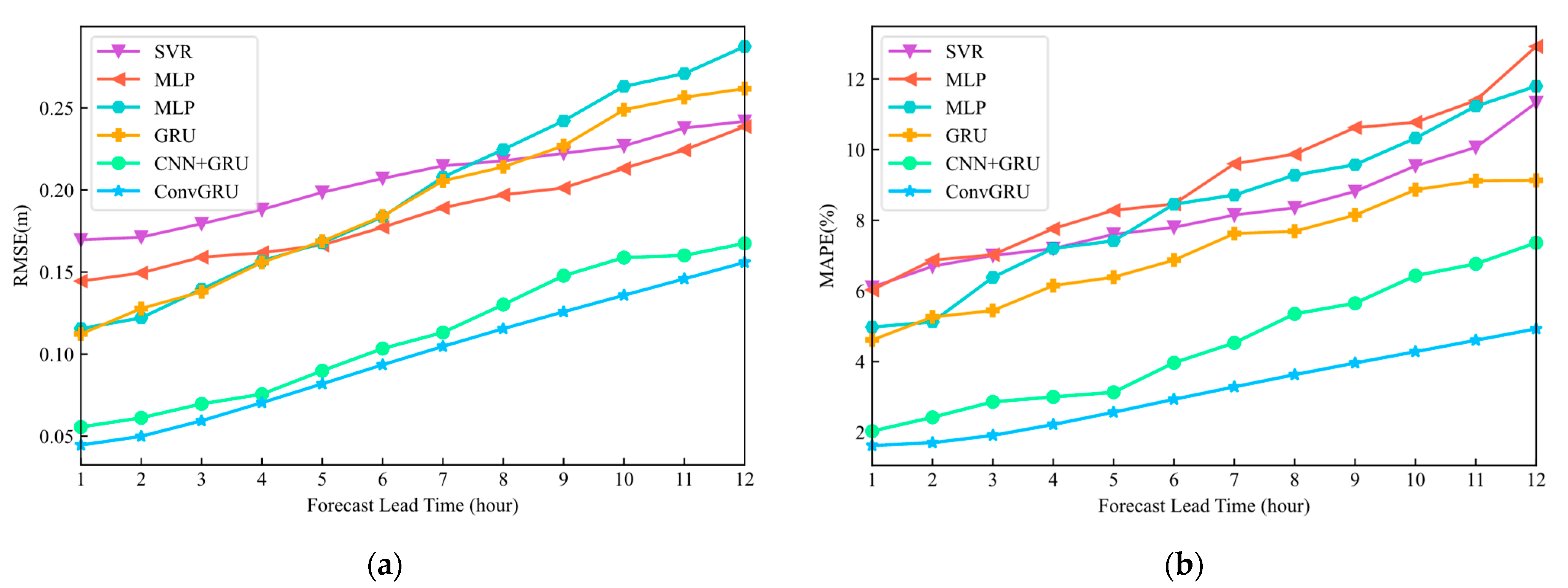
SVR is a form of SVM applied to regression problems. SVR treats the regression problem as an optimization problem by constructing a hyperplane that minimizes the distance to sample points in the sample space. However, unlike the general regression model, SVR incorporates fault tolerance for outlier samples to improve generalization [38,39]. In the experiments, SVR uses an rbf kernel with kernel coefficients taken as the reciprocal of the number of sample features and a penalty parameter of 1. Multi-step prediction is achieved using the DMS strategy.

(2)

MLP has good nonlinear regression because it can theoretically approximate any nonlinear function through the nonlinear activation of multilayer neurons and the fully connected structure [24,25]. Moreover, the fully connected structure enables the MLP to perform multi-step prediction using the MIMO strategy. The MLP uses three network layers with 200, 400, and 12 neurons in the experiment.

(3)

LSTM is a classical RNN model that uses a gating mechanism to control the forgetting and selection of memory states [18]. Unlike GRU, LSTM has two states. The cell state is responsible for preserving the long-term information of the time series, and the hidden state is the output on the current time step. To handle both states, the LSTM has one more control gate than the GRU and thus has a larger number of parameters for the same setup. The network structure used is a single LSTM layer—Dropout layer—fully connected output layer. The LSTM layer size is 400, and the tanh activation function is used. The Dropout layer discard rate is 0.2, and the fully connected layer size is 12, using linear activation. The model is trained at batch size = 32, learning rate = 0.0001.

(4)

GRU enables the transfer of information memory between time steps through a circular connection structure along the time axis. GRU not only captures the temporal correlation between multidimensional time series efficiently but also has a faster training speed than LSTM [40]. Since the structure of LSTM and GRU is more similar, the same grid structure and training hyperparameters as LSTM are used for GRU in the experiments.

(5)

CNN+GRU adds a convolutional layer shared on the time axis to GRU to achieve successive extraction of spatial and temporal structures. At each time step, the spatial features are extracted using the convolutional layer to transform the input information of a single moment into a one-dimensional sequence containing spatial information. Thereafter, the temporal structure of the one-dimensional sequence at each moment is extracted using GRU, and the single-step regional prediction results are output.

The error values of the comparison experiment at 12 moments and the average values are shown in

Table 5. Error experimental results of model comparison experiments.

Model	Error	1	2	3	4	5	6	7	8	9	10	11	12	Mean
SVR	RMSE	0.1696	0.1713	0.1795	0.1881	0.1986	0.2071	0.2148	0.2178	0.2224	0.2269	0.2378	0.2419	0.2063
	MAE	0.1576	0.1612	0.1676	0.1838	0.1912	0.2043	0.2069	0.2096	0.2143	0.2208	0.2249	0.2284	0.1976
	MAPE	6.1076	6.6984	7.0042	7.1985	7.6037	7.8020	8.1490	8.3553	8.8201	9.5414	10.0658	11.3289	8.2229
MLP	RMSE	0.1445	0.1495	0.1591	0.1618	0.1665	0.1773	0.1892	0.1971	0.2013	0.2132	0.2244	0.2387	0.1852
	MAE	0.1292	0.1398	0.1449	0.1456	0.1575	0.1692	0.1755	0.1813	0.1950	0.2018	0.2144	0.2257	0.1733
	MAPE	6.0294	6.8732	7.0264	7.7628	8.2841	8.4627	9.6008	9.8731	10.6233	10.7755	11.3936	12.9243	9.1358
LSTM	RMSE	0.1156	0.1221	0.1396	0.1568	0.1678	0.1837	0.2079	0.2247	0.2422	0.2632	0.2710	0.2875	0.1985
	MAE	0.1126	0.1298	0.1396	0.1407	0.1586	0.1662	0.1689	0.1725	0.1885	0.2156	0.2259	0.2338	0.1717
	MAPE	4.9765	5.1250	6.3860	7.2080	7.4165	8.4579	8.7160	9.2815	9.5755	10.3267	11.2312	11.7987	8.3750
GRU	RMSE	0.1123	0.1278	0.1380	0.1559	0.1688	0.1841	0.2056	0.2141	0.2270	0.2489	0.2565	0.2619	0.1917
	MAE	0.0999	0.1146	0.1219	0.1361	0.1442	0.1550	0.1727	0.1765	0.1866	0.2053	0.2107	0.2137	0.1614
	MAPE	4.6107	5.2614	5.4458	6.1504	6.3911	6.8728	7.6227	7.6893	8.1477	8.8649	9.1178	9.1318	7.1089
CNN+GRU	RMSE	0.0556	0.0612	0.0697	0.0756	0.0899	0.1034	0.1132	0.1302	0.1478	0.1589	0.1602	0.1675	0.1111
	MAE	0.0421	0.0496	0.0509	0.0631	0.06716	0.0705	0.0891	0.0951	0.1205	0.1321	0.1406	0.1489	0.0891
	MAPE	2.0321	2.4231	2.8621	3.0012	3.1326	3.9682	4.5312	5.3521	5.6531	6.4325	6.7675	7.3654	4.4600
Conv GRU	RMSE	0.0446	0.0499	0.0594	0.0704	0.0819	0.0935	0.1047	0.1155	0.1258	0.1359	0.1459	0.1559	0.0986
	MAE	0.0345	0.0372	0.0428	0.0501	0.0583	0.0667	0.0748	0.0826	0.0902	0.0975	0.1049	0.1122	0.0710
	MAPE	1.6250	1.7045	1.9111	2.2194	2.5661	2.9332	3.2848	3.6306	3.9610	4.2808	4.6043	4.9291	3.1375

. The error curve plots of the comparison experiments at 12 moments are shown in Figure 9. Since the MAE curve is similar to the RMSE curve, only the RMSE and MAPE plots are shown in the image.

As can be seen from Figure 9, the error of each model gradually increases with the delay of the prediction moment. Among them, the errors of SVR, MLP, LSTM, and GRU are higher at each moment, significantly higher than CNN+GRU and ConvGRU, indicating that the missing spatial information greatly increases the errors of spatio-temporal series prediction. It leads to low accuracy of regional wave height prediction. In the approaching moments from 1–6 h, the CNN+GRU errors and ConvGRU errors are similar, and both errors are relatively low. However, starting from 6 h, the MAPE error of CNN+GRU is higher, and the RMSE and MAE error errors are lower in the leaning moments, but the overall errors of CNN+GRU are both lower than those of MLP and GRU. The results show that ConvGRU exhibits the lowest error in MAPE, MAE, and RMSE errors at all moments compared with the other three models, and the average error at all moments is also the lowest, which proves the superior multi-step prediction performance of ConvGRU for spatio-temporal sequences.

As can be seen from Table 5, ConvGRU has the lowest average of all three metrics and is the best model (Marked in bold in Table 5), while CNN+GRU ranks second and is the second-best model. Compared with the CNN+GRU model, the average values of RMSE, MAE, and MAPE at 12 moments were reduced by 11.25%, 20.31%, and 29.65%, respectively, for the model using ConvGRU and the multiple-input multiple-output strategy.

To evaluate in more detail the predictability of the regional multi-step wave height prediction model based on the ConvGRU network compared to other models, Figure 10 shows the true value-predicted value scatter density distribution of 3486 prediction samples under different models of SVR, MLP, LSTM, GRU, CNN+GRU, and ConvGRU, which predicted a total of 2,677,247 (3486 * 12 * 8 * 8) wave height values, and because of the large number of predictions, one is taken every 50 prediction points. It is obvious from Figure 10 that using SVR, MLP, and LSTM models appear to have several points with large prediction point errors, while the GRU model has small errors in most of the prediction points. The overall errors of SVR, MLP, LSTM, and GRU time series prediction methods are large, indicating that it is not good practice to use input data with loss of spatial correlation to predict regional wave heights at a single moment in time. The CNN+GRU method has a small number of prediction points with small errors, but the errors are much smaller than those of the time series methods due to the inclusion of spatial information. The error of the regional multi-step prediction model based on ConvGRU proposed in this paper is small overall, and the predicted and true values of the prediction points are close to each other, and the prediction accuracy is significantly improved.

4.6. Applicability of the Model

Considering that the model needs to be used for medium to large wave forecasting and needs to adapt to different wave areas, two wave areas, C and D, are randomly selected in this paper. The spatial and temporal series of the wave height, wave direction, and wave period for the period of 2020–2021 were extracted from ERA5, containing 17,544 h of data. The maximum value, mean, variance, and standard deviation of wave heights in the sea area and the results of wave height prediction errors obtained under the model of this paper are shown in

Table 6. Information and error results for different sea areas.

Sea Areas	MAX (m)	MEAN (m)	VAR (m2)	STD (m)	MRMSE	MMAE	MMAPE
C	3.5578	1.5766	0.2450	0.4950	0.0814	0.0631	4.2154
D	5.0784	2.2308	0.3066	0.5538	0.1248	0.0862	3.9586
Original	5.9778	2.2551	0.4121	0.6420	0.0986	0.0710	3.1375

. Despite the slight increase in errors, the model has low errors in all regions and can achieve high accuracy regional prediction.

5. Conclusions

In this paper, we propose a model with ConvGRU as the main body and a multi-input, multioutput, and multi-step prediction strategy for the sea surface wave height multi-step spatio-temporal prediction problem. The model can better capture the global spatial information and map it to the desired multi-location output and can learn different prediction moment samples simultaneously to achieve accurate spatio-temporal prediction. In addition, this paper also improves the ConvGRU model by adding wave direction and wave period exogenous variables to the input using the Leaky ReLU activation function, and these improvements are proven to be effective. The paper presents a novel wave height prediction model based on ConvGRU, which makes significant contributions in several areas. Firstly, the proposed model addresses the challenges of multi-location and multi-step prediction in wave height forecasting, which is not possible with traditional models. Secondly, the model achieves low prediction errors even for long-term predictions, which is important for applications such as marine operations and meteorological hydrological support.

In summary, the paper’s contributions demonstrate the effectiveness of the proposed ConvGRU-based model for wave height prediction in multiple locations and steps, with potential applications in ocean engineering, marine operations, and other related fields.

The limitation of this paper is that it only focuses on predicting waves in regions that are significant for global crude oil transportation routes. In the future, the paper intends to expand the prediction area and duration beyond these regions.

References

- Chen, C.; Shiotani, S. Numerical ship navigation based on weather and ocean simulation. Ocean Eng. 2013, 69, 44–53. [Google Scholar] [CrossRef]
- Chen, B.; Kou, Y.; Wang, Y.; Zhao, D.; Liu, S.; Liu, G.; Han, X. Analysis of storm surge characteristics based on stochastic process. AIMS Math. 2021, 6, 1177–1190. [Google Scholar] [CrossRef]
- Chen, C.; Sasa, K. Statistical analysis of waves’ effects on ship navigation using high-resolution numerical wave simulation and shipboard measurements. Ocean Eng. 2021, 229, 108757. [Google Scholar] [CrossRef]
- Camus, P.; Losada, I.; Izaguirre, C.; Espejo, A.; Menéndez, M.; Pérez, J. Statistical wave climate projections for coastal impact assessments. Earth’s Future 2017, 5, 918–933. [Google Scholar] [CrossRef]
- Camus, P.; Menendez, M.; Mendez, F.J.; Izaguirre, C.; Espejo, A.; Canovas, V.; Perez, J.; Rueda, A.; Losada, I.J.; Medina, R. A weather-type statistical downscaling framework for ocean wave climate. J. Geophys. Res. Ocean. 2014, 119, 7389–7405. [Google Scholar] [CrossRef]
- Soman, S.S.; Zareipour, H.; Malik, O.; Mandal, P. A review of wind power and wind speed forecasting methods with different time horizons. In Proceedings of the North American Power Symposium, Arlington, TX, USA, 26–28 September 2010; pp. 1–8. [Google Scholar] [CrossRef]
- Bridges, T.J. Waves in Oceanic and Coastal Waters. Q. J. R. Meteorol. Soc. 2008, 134, 1947–1948. [Google Scholar] [CrossRef]
- Booij, N.; Ris, R.C.; Holthuijsen, L.H. A third-generation wave model for coastal regions: 1. Model description and validation. J. Geophys. Res. Ocean. 1999, 104, 7649–7666. [Google Scholar] [CrossRef]
- Mentaschi, L.; Besio, G.; Cassola, F.; Mazzino, A. Performance evaluation of Wavewatch III in the Mediterranean Sea. Ocean Model. 2015, 90, 82–94. [Google Scholar] [CrossRef]
- Rogers, W.E.; Hwang, P.A.; Wang, D.W. Investigation of wave growth and decay in the SWAN model: Three Regional-Scale applications. J. Phys. Oceanogr. 2003, 33, 366–389. [Google Scholar] [CrossRef]
- Samiksha, S.V.; Jancy, L.; Sudheesh, K.; Kumar, V.S.; Shanas, P.R. Evaluation of wave growth and bottom friction parameterization schemes in the SWAN based on wave modelling for the central west coast of India. Ocean Eng. 2021, 235, 109356. [Google Scholar] [CrossRef]
- Bingölbali, B.; Jafali, H.; Akpınar, A.; Bekiroğlu, S. Wave energy potential and variability for the south west coasts of the Black Sea: The WEB-based wave energy atlas. Renew. Energy 2020, 154, 136–150. [Google Scholar] [CrossRef]
- Li, A.; Guan, S.; Mo, D.; Hou, Y.; Hong, X.; Liu, Z. Modeling wave effects on storm surge from different typhoon intensities and sizes in the South China Sea. Estuar. Coast. Shelf Sci. 2020, 235, 106551. [Google Scholar] [CrossRef]
- Zhou, W.; Shan, D.; Yang, J. The Modeling of Interval-Valued Time Series: A Method Based on Fuzzy Set Theory and Artificial Neural Networks. Int. J. Comput. Intell. Appl. 2019, 18, 1950002. [Google Scholar] [CrossRef]
- Jäger, W.S.; Nagler, T.; Czado, C.; McCall, R.T. A Statistical Simulation Method for Joint Time Series of Non-Stationary Hourly Wave Parameters. Coast. Eng. 2019, 146, 14–31. [Google Scholar] [CrossRef]
- Asma, S.; Sezer, A.; Ozdemir, O. MLR and ANN models of significant wave height on the west coast of India. Comput. Geosci. 2012, 49, 231–237. [Google Scholar] [CrossRef]
- Makarynskyy, O.; Pires-Silva, A.A.; Makarynska, D.; Ventura-Soares, C. Artificial neural networks in wave predictions at the west coast of Portugal. Comput. Geosci. 2005, 31, 415–424. [Google Scholar] [CrossRef]
- Gao, S.; Huang, J.; Li, Y.; Liu, G.; Bi, F.; Bai, Z. A forecasting model for wave heights based on a long short-term memory neural network. Acta Oceanol. Sin. 2021, 40, 62–69. [Google Scholar] [CrossRef]
- Choi, H.; Park, M.; Son, G.; Jeong, J.; Park, J.; Mo, K.; Kang, P. Real-time significant wave height estimation from raw ocean images based on 2D and 3D deep neural networks. Ocean Eng. 2020, 201, 107129. [Google Scholar] [CrossRef]
- Zhou, S.; Xie, W.; Lu, Y.; Wang, Y.; Zhou, Y.; Hui, N.; Dong, C. ConvLSTM-Based wave forecasts in the South and East China Seas. Front. Mar. Sci. 2021, 8, 740. [Google Scholar] [CrossRef]
- Liu, X.; Zhang, H.; Kong, X.; Lee, K.Y. Wind speed forecasting using deep neural network with feature selection. Neurocomputing 2020, 397, 393–403. [Google Scholar] [CrossRef]
- Gu, C.; Li, H. Review on Deep Learning Research and Applications in Wind and Wave Energy. Energies 2022, 15, 1510. [Google Scholar] [CrossRef]
- Song, T.; Han, R.; Meng, F. A significant wave height prediction method based on deep learning combining the correlation between wind and wind waves. Front. Mar. Sci. 2022, 9, 983007. [Google Scholar] [CrossRef]
- James, S.C.; Zhang, Y.; O’Donncha, F. A machine learning framework to forecast wave conditions. Coast. Eng. 2018, 137, 1–10. [Google Scholar] [CrossRef]
- Feng, X.; Ma, G.; Su, S.F.; Huang, C.; Boswell, M.K.; Xue, P. A multi-layer perceptron approach for accelerated wave forecasting in Lake Michigan. Ocean Eng. 2020, 211, 107526. [Google Scholar] [CrossRef]
- Pirhooshyaran, M.; Snyder, L.V. Forecasting, hindcasting and feature selection of ocean waves via recurrent and sequence-tosequence networks. Ocean Eng. 2020, 207, 107424. [Google Scholar] [CrossRef]
- Yu, J.; Lu, Z.; Wei, H. Numerical study of a CNN-based model for regional wave prediction. Ocean Eng. 2022, 255, 111400. [Google Scholar] [CrossRef]
- Vandenhende, S.; Georgoulis, S.; Van Gansbeke, W.; Proesmans, M.; Dai, D.; Van Gool, L. Multi-task learning for dense prediction tasks: A survey. IEEE Trans. Pattern Anal. Mach. Intell. 2022, 44, 3614–3633. [Google Scholar] [CrossRef]
- Liu, J.; Xu, L.; Chen, N. A spatiotemporal deep learning model ST-LSTM-SA for hourly rainfall forecasting using radar echo images. J. Hydrol. 2022, 609, 127748. [Google Scholar] [CrossRef]
- Shi, X.; Chen, Z.; Wang, H.; Yeung, D.Y.; Wong, W.K.; Woo, W.C. Convolutional LSTM network: A machine learning approach for precipitation nowcasting. In Proceedings of the 28th International Conference on Neural Information Processing Systems, Montreal, QC, Canada, 7–12 December 2015; pp. 802–810. [Google Scholar]
- Ben Taieb, S.; Bontempi, G.; Atiya, A.F.; Sorjamaa, A. A review and comparison of strategies for multi-step ahead time series forecasting based on the NN5 forecasting competition. Expert Syst. Appl. 2012, 39, 7067–7083. [Google Scholar] [CrossRef]
- Carr, C.M.; Yavary, M.; Yavary, M. Wave agitation studies for port expansion-Salalah, Oman. In Proceedings of the Ports 2004: Port Development in the Changing World, Houston, TX, USA, 23–26 May 2004; pp. 1–10. [Google Scholar]
- Anoop, T.R.; Kumar, V.S.; Shanas, P.R.; Johnson, G. Surface Wave Climatology and Its Variability in the North Indian Ocean Based on ERA-Interim Reanalysis. J. Atmos. Oceans Technol. 2015, 32, 1372–1385. [Google Scholar] [CrossRef]
- Rashmi, R.; Aboobacker, V.; Vethamony, P.; John, M. Co-existence of wind seas and swells along the west coast of India during non-monsoon season. Ocean Sci. 2013, 9, 281. [Google Scholar] [CrossRef]
- Wang, J.; Wang, Y.; Yang, J. Forecasting of significant wave height based on gated recurrent unit network in the Taiwan strait and its adjacent waters. Water 2021, 13, 86. [Google Scholar] [CrossRef]
- Zhang, D.; Kabuka, M.R. Combining Weather Condition Data to Predict Traffic Flow: A GRU Based Deep Learning Approach. IET Intell. Transp. Syst. 2018, 12, 578–585. [Google Scholar] [CrossRef]
- Dai, G.; Ma, C.; Xu, X. Short-term Traffic Flow Prediction Method for Urban Road Sections Based on Space-time Analysis and GRU. IEEE Access 2019, 7, 143025–143035. [Google Scholar] [CrossRef]
- Fan, S.; Xiao, N.; Dong, S. A novel model to predict significant wave height based on long short-term memory network. Ocean Eng. 2020, 205, 107298. [Google Scholar] [CrossRef]
- Mahjoobi, J.; Adeli, E. Prediction of significant wave height using regressive support vector machines. Ocean Eng. 2009, 36, 339–347. [Google Scholar] [CrossRef]
- Liu, X.; Lin, Z.; Feng, Z. Short-term offshore wind speed forecast by seasonal ARIMA—A comparison against GRU and LSTM. Energy 2021, 227, 120492. [Google Scholar] [CrossRef]