1. Introduction
High-speed railway is the common trend of railway transportation development in the world, and is the main symbol of railway technology modernization [
1,
2,
3,
4]. Rapid economic development and increasing urbanization rate have put forward higher requirements for the operational efficiency of high-speed railways. Improving the line utilization rate is one of the key technologies that can improve train operation efficiency, and puts forward higher requirements and challenges for the driving strategy of high-speed trains.
With the continuous improvement of train control automation, the driver’s subjectivity in the process of train running is decreasing, and the driving mode is undergoing transformation between manual driving, semi-automatic driving, automatic driving, and fully automatic driving. The automatic driving technique is a hot research topic for trains both at home and abroad [
5,
6,
7,
8,
9,
10]. In [
6], based on the Cerebellar Model Articulation Controller (CMAC) adaptive control law, a train optimization control algorithm is proposed which can overcome the overkill phenomenon and poor convergence problems of the conventional PID while to a certain extent reducing the influence of parameter uncertainty and external interferences. In [
7], an intelligent driving algorithm was put forward to compensate for nonlinear disturbances, relying on fractional-order sliding mode adaptive control and neural networks. In [
8], a neural adaptive driving strategy was proposed for high-speed trains subject to unknown parameters and bounded disturbances. The above research is based on the single-mass point model. In [
9,
10], high-speed trains were modeled as a multiple-mass point model. For the sake of obtaining good position tracking performances and velocity tracking performance, the composite driving strategy and the neural adaptive driving strategy have been proposed. In the former, the tracking control problem of high-speed trains with the base running resistances and the external wind is transformed into a stabilization problem of linear systems with the modeled disturbance and the norm-bounded disturbance. In the latter, the tracking control problem of high-speed trains with the base running resistances and the external additional resistances is transformed into the arrival problem of sliding mode surfaces with time-varying coefficients.
In modern society, high-speed trains have the characteristics of high running density and long driving cycles. The automation driving control of a certain train is determined both by its own running conditions and the relationship that it has with adjacent trains on the same line. If the train can obtain the information of adjacent vehicles, it can achieve better performance. As a consequence, cooperative control for multiple high-speed trains is becoming a research trend [
11,
12,
13,
14,
15,
16,
17,
18,
19]. Based on comparison of the minimum tracking interval time under fixed automatic block, quasi-moving block, and moving block conditions, Hill and Bond established the moving block railway signal system model, then analyzed the advantages of moving block for multiple high-speed trains [
12]. However, it is obvious that cooperation control for multiple high-speed trains with fixed automatic block or quasi-moving block has certain limitations; a cooperation driving scheme with moving block can effectively improve the cooperation performances between trains while ensuring a safe interval between adjacent trains. Moreover, the utilization rate and operation efficiency of the line can be improved without sacrificing safety. In [
14], the authors discuss the cooperation control problem for multiple high-speed trains with moving block. In [
15], the limitation problem between the running speed and the traction/braking force is addressed for multiple high-speed trains with bounded disturbances. The saturation truncation function is applied to deal with the constraint of the traction/braking force, and the speed constraint function is introduced to deal with the constraint of velocity. Then, a fuzzy logic adaptive cooperation control algorithm is proposed to realize the cooperative operation of multiple high-speed trains. Virtual coupling (see
Figure 1a) is a new moving block technology which relies on information exchange between trains. In [
16], Dong et al. proposed a cooperation driving strategy based on information between adjacent trains. In [
17], Cao et al. presented a cooperation control scheme with an anti-collision mechanism for multiple high-speed trains, taking the Beijing–Shanghai high-speed railway as an example. Their approach is based on the time-varying parameter artificial potential field function, and they verified the feasibility and effectiveness of the proposed cooperation driving strategy. In [
19], Tian and Lin proposed a cooperative driving algorithm for multiple high-speed trains with moving block. To reduce the cost of operation adjustment and communication between trains, a switching mechanism and acceleration zone were applied.
Based on the above analysis, higher requirements and challenges can be put forward for cooperative driving strategies with moving block. In most existing research on multiple high-speed trains, each train follows its own curve of displacement and speed (see
Figure 1b). It is obvious that there is no real-time communication between the trains. Consequently, in this paper the cooperation control problem for multiple high-speed trains with moving block is addressed, as shown in
Figure 1a. Unlike the existing train cooperation operations shown as
Figure 1b, the controller in this paper ensures that the position and velocity of the first train can track the given displacement and velocity curves well. Meanwhile, for the other trains, their desired velocity curves are viewed as the real-time speed of the adjacent front train, and the ideal safety interval between the adjacent trains can be maintained; in this way, a good line utilization rate can be obtained by the cooperation controller presented in this paper. First, multiple high-speed trains can be modeled as a quasi multi-agent system with parametric uncertainty. Then, the non-singular terminal sliding mode surfaces are introduced to transform the tracking control problem into the arrival problem. Next, the adaptive laws are designed to estimate the unknown parameters and the bounded disturbance. Following sliding mode surfaces and adaptive laws, a dual jitter suppression mechanism can be achieved. Finally, Lyapunov stability theory is applied to prove the stability of the system, and simulation results show that the proposed cooperation control strategy is effective and feasible. Meanwhile, in order to enrich the proposed control algorithm, the adaptive laws are rewritten without leakage terms. Moreover, the case of multiple high-speed trains with known parameters is discussed. Generally speaking, compared with existing research results, the main contributions of this paper can be summed up as follows:
Real-time communication is carried out between the rear train and the adjacent front train. The real-time displacement and speed of the front train are taken as the reference to adjust its own running state in real time. Under this operation mode, multiple high-speed trains can be modeled as a quasi-multi-agent system using the leader–follower model.
A novel cooperation control scheme is applied to multiple high-speed trains with parametric uncertainty and multiple disturbances, which is effective and feasible for improving the line utilization rate.
The dual jitter suppression mechanism is designed, which relies on the non-singular terminal sliding mode control and the adaptive control. The adaptive laws with leakage terms is designed to compensate the unknown parameters, parametric uncertainty, and bounded disturbances.
The rest of this paper is organized as follows. Based on
Section 2, which describes the dynamic model of multiple high-speed trains subject to multiple disturbances, in
Section 3 the adaptive laws are applied to estimate the unknown parameters and unknown bounded disturbances and the stability of the system is proven by reference to Lyapunov theory. In addition, two corollaries are proposed for multiple high-speed trains. The effectiveness and feasibility of the proposed terminal sliding mode cooperation control scheme is verified by simulation results in
Section 4. Finally, in
Section 5 the paper is summarized and our conclusions are provided.
2. Dynamics Modeling
Based on the single-point mass model [
20,
21,
22], the following dynamical model for multiple high-speed trains subject to multiple disturbances is designed:
where
and
are the position and velocity, respectively;
denote the total mass and satisfy
;
are bounded and imply the uncertainty of the dynamics model;
are positive parameters;
represent the control input, i.e., the traction force or the braking force; and
and
are the base running resistances and external additional resistances, respectively. The former can be viewed as the modeled disturbance, and can be formulated as
; Davis’ coefficients
,
, and
are unknown uncertain parameters, and satisfy
,
, and
, where
,
,
are positive constants; and
,
,
reflect the uncertainty of Davis’ coefficients. The latter can be viewed as the bounded disturbances, and consist of the ramp resistance, the tunnel resistances, the curve resistance, etc.
Remark 1. As shown in Equation (1), the single-point mass model, with the advantages of simple structure and easy implementation, is applied to describe the dynamical model for multiple high-speed trains. Hence, it can be widely used in the problem of the dynamical model and cooperation controller design for multiple high-speed trains. However, the multiple-point mass model has the disadvantages of complex structure and large amount of calculation; nonetheless, it can better reflect the force and operation of the train and is closer to the actual train model. Remark 2. In this paper, the dynamic model of multiple high-speed trains subject to the base running resistances and the external additional resistances is designed. Meanwhile, the relevant parameters, i.e., the total mass and Davis’ coefficients are unknown and uncertain, which is more in line with the actual operation of multiple high-speed trains.
Moreover, Equation (
1) can be rearranged as
where
. Without loss of generality, the functions
are bounded. Then, there exist positive constants
which satisfy the inequalities
.
Remark 3. In Equation (1), the bounded parameters , , , imply the parameter uncertainty. Consequently, there exist positive parameters satisfying . Through combination with the boundedness of , we can find the parameters to ensure that the inequation is true, that is to say, that the assumptions are reasonable. Based on virtual coupling,
i = 1 is designed to be the leading train. Then, the leader–follower model can be designed between train
i and train
i−1. When
i = 1, the leader–follower model can be designed between the leading train and its desired tracking curves. In this paper, the major objective is to design a cooperation control scheme that can ensure good tracking and cooperation performance for multiple high-speed trains subject to parametric uncertainty. In order to achieve the above objective, the following errors are designed:
where
is the safe interval between the adjacent trains,
and
are the position tracking errors and velocity tracking errors, respectively, and
and
are the desired position curve and velocity curve of the leading train, respectively.
Remark 4. Based on Figure 1, the safe interval between the adjacent trains in this paper is superior, and can improve the utilization rate of the line to an extent. However, the ideal safe interval is defined as a constant, which is a drawback of the presented control algorithm. In our future research, we intend to solve this problem. Assumption 1. The desired position of the leading train is assumed to be a known smooth function, i.e., , , and can be viewed as bounded functions.
Combining Equations (
2) and (
3), we have
where
is the desired acceleration of the leading train and
represents the acceleration of train
(
).
3. Cooperation Controller Design and Stability Analysis
In this section, for sake of transforming the tracking control problem and cooperation control problem into the arrival problem of the sliding mode surfaces, the following terminal sliding mode surfaces are proposed for multiple high-speed trains subject to parametric uncertainty:
where
and
and
are positive odd constants, and satisfy
. Hence, we have
On the basis of (
2), (
3), and (
6), the following cooperation control strategy is presented to obtain the desired performance:
where
represents the controller gains, which can be obtained from empirical values;
,
,
,
and
are the estimates of
,
,
,
, and
; and the disturbance compensation can be designed as
.
Based on the above analysis, we can draw the following theorem:
Theorem 1. Given the dynamical model (2) and the sliding mode surfaces (5), if the adaptive laws of unknown parameters , , , , and are designed aswhere , , , , and denote the adaptive parameters, and , , , , and denote the leakage parameters, then the system with the controller in Equation (7) is exponentially stable. Thus, the desired safe interval between adjacent trains can be maintained, and the cooperation performances for multiple high-speed trains can be obtained. Proof. To ensure the desired performance of multiple high-speed trains subject to parametric uncertainty, we construct the following Lyapunov function:
with
where
,
,
,
, and
are the error terms of the unknown parameters, and satisfy
By substituting Equations (
4) and (
6) into the above formula (
11), we have
By combining this with the controller in Equation (
7) and the adaptive laws in Equation (
8), Equation (
12) can be further arranged as
Moreover, Equation (
13) can be rewritten as
Given
,
,
,
, and
, we have
,
,
,
,
, which together imply the following inequalities:
Consequently, Equation (
14) can be rewritten as
Furthermore, through Equations (
9), (
10), and (
16), we can derive
where
. The parameters
,
,
,
, and
and the leakage coefficients
,
,
,
, and
are bounded; thus,
is a bounded function. Therefore, a parameter
exists which satisfies
; the parameter
can be designed to satisfy the following equations:
,
,
,
,
,
. Consequently, we have
Furthermore, through Equations (
9), (
10), and (
16), we can derive
where
;
. Combining this with Equations (
9), (
10), and (
17), we have [
23]
where
,
. Then, the boundary of the sliding mode surface
and the parameter errors
,
,
,
,
can be obtained:
Based on this analysis, it is readily obtained that , , , , , and can converge to a very small area near zero. Thus, the system is exponentially stable for multiple high-speed trains with the proposed cooperation control scheme. The proposed control algorithm is proven to be feasible and efficient, and can ensure the desired tracking and cooperation performance. □
However, it is difficult to solve the convergence time under the terminal sliding mode surfaces-based cooperative control strategy [
24]. By means of Equations (
5), (
9), (
10), (
16), and (
17), when the following inequality is assumed
we obtain
where
and
is the time to reach the sliding mode surface from the initial state for the system, and satisfies
Through Equation (
5), the time
to reach the origin along the sliding mode surface for the system can be calculated as
Consequently, we can obtain the convergence time of the system as .
Remark 5. Based on the cooperation control scheme proposed in this paper, the arrival time is subject to the above assumption.
Remark 6. In this paper paper, train i asymptotically tracks the speed of train i-1 by means of the proposed cooperation control schemes, allowing a safe interval to be maintained between two adjacent trains. However, when i=1, the leading train follows a given displacement and velocity curve.
Remark 7. The cooperation control problem of multiple high-speed trains subject to parameter uncertainty is investigated in Theorem 1. The unknown and uncertain parameters are divided into the unknown positive constant and the uncertainty. The latter is viewed as the unknown bounded term. Combined with the base running resistances and the extra additional resistances, the latter can be compensated for by the adaptive control. Based on the adaptive control, the cooperation control scheme is proposed.
Theorem 1 is presented for multiple high-speed trains with unknown parameters and leakage terms. In addition, the following conclusions can be obtained.
Corollary 1. Considering the dynamical model (2) and the sliding mode surfaces (5), if the adaptive laws of unknown parameters , , , , and are designed aswhere , , , , and denote the adaptive parameters, then the proposed controller in Equation (7) is effective and feasible. Moreover, multiple high-speed trains are able to reach the desired cooperation and tracking performance. Proof. Based on the proof of Theorem 1, substituting the proposed controller (
7) and the unknown parameter adaptive laws (
18) into Equation (
12) yields
Moreover, Equation (
19) can be rearranged as
Considering
,
and Equations (
9) and (
10), we have
. In combination with Lyapunov theory, the presented cooperation control scheme can ensure the desired cooperation and tracking performance. □
Corollary 2. Considering the dynamical model (2) with the known parameters , , , , and , based on the sliding mode surfaces (5), the cooperation controller for multiple high-speed trains can be presented as follows:where , , and are the known parameters and . Then, multiple high- speed trains are able to reach the desired cooperation and tracking performance. Proof. To prove the effectiveness and feasibility of the proposed control strategy (
20), the following Lyapunov function can be designed:
which implies that
. Combining this with Equations (
4), (
6) and (
20)
can be rearranged as
Then, based on the the proof of Corollary 1, the proposed cooperation control scheme in Corollary 2 is proven to be effective and feasible. Thus, multiple high-speed trains with the proposed control scheme (
20) can obtain the desired tracking and cooperation performance. □
Remark 8. The difference between Theorem 1 and Corollary 1 lies in the adaptive laws (8) and (18). Meanwhile, the difference between Theorem 1 and Corollary 2 is the dynamical model. To be more specific, the dynamical model with unknown parameters is considered in Theorem 1, and the dynamical model with known parameters is considered in Corollary 2. However, the proofs of Corollary 1 and Corollary 2 can be derived from the proof of Theorem 1. Consequently, we reduced the proofs of Corollary 1 and Corollary 2. Remark 9. As shown in [25,26,27], the stability of the tracking error and its corresponding derivative can be proven. On the basis of the terminal sliding mode surfaces (5), it is obvious that we can obtain the variables of the terminal sliding mode surfaces, which are the tracking error and it corresponding derivative. Combining this with the Assumption 1, we can find the stability of the tracking error and its corresponding derivative. 4. Simulation Results
In this section, a simulation experiment for multiple high-speed trains with is carried out. The train parameters are designed as follows: , , , , .
The external additional resistances
are defined as
where
and
are the bend length and the rail length, respectively; the center corner of the bend is
; the ramp angle is
; and the parameter uncertainty is chosen as
,
,
,
, where
represents a random number between 0 and 1.
We design the safe interval between the adjacent trains as . The sliding mode surface coefficients, cooperation controller coefficients, adaptive law coefficients, and leakage coefficients are chosen by means of the empirical values: , , , , , , , , , , , , , , , , , , , , , , , , , , , .
Based on the above conditions, the simulation results are shown in
Figure 2,
Figure 3,
Figure 4,
Figure 5,
Figure 6 and
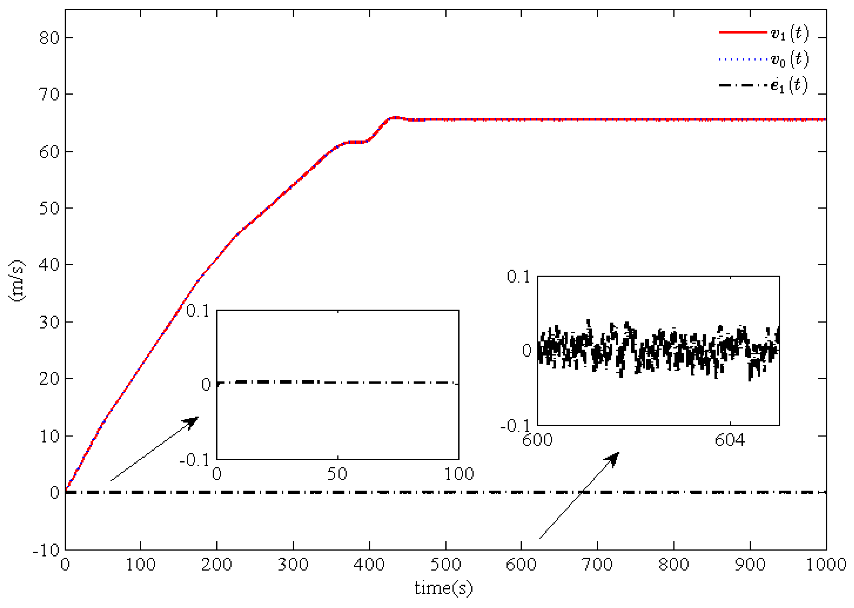
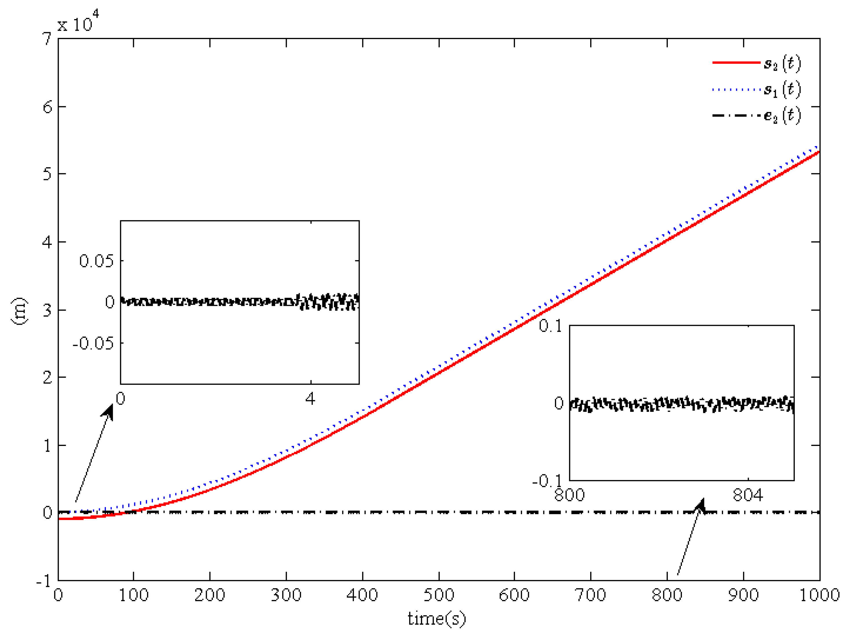
Figure 7, where
Figure 2,
Figure 4 and
Figure 6 show the actual position curves
, the desired position curves
, and the position tracking error curves
for trains
and
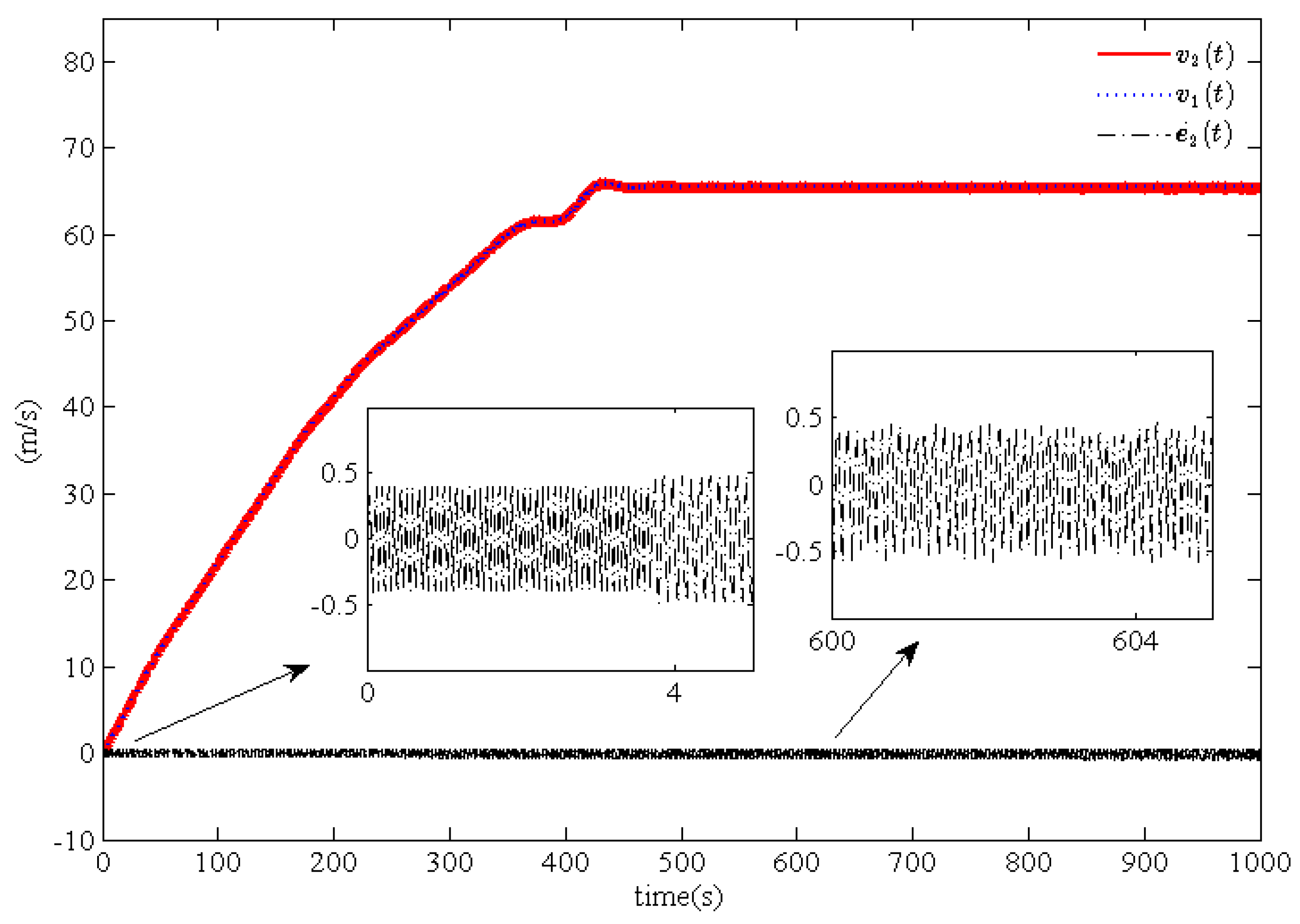
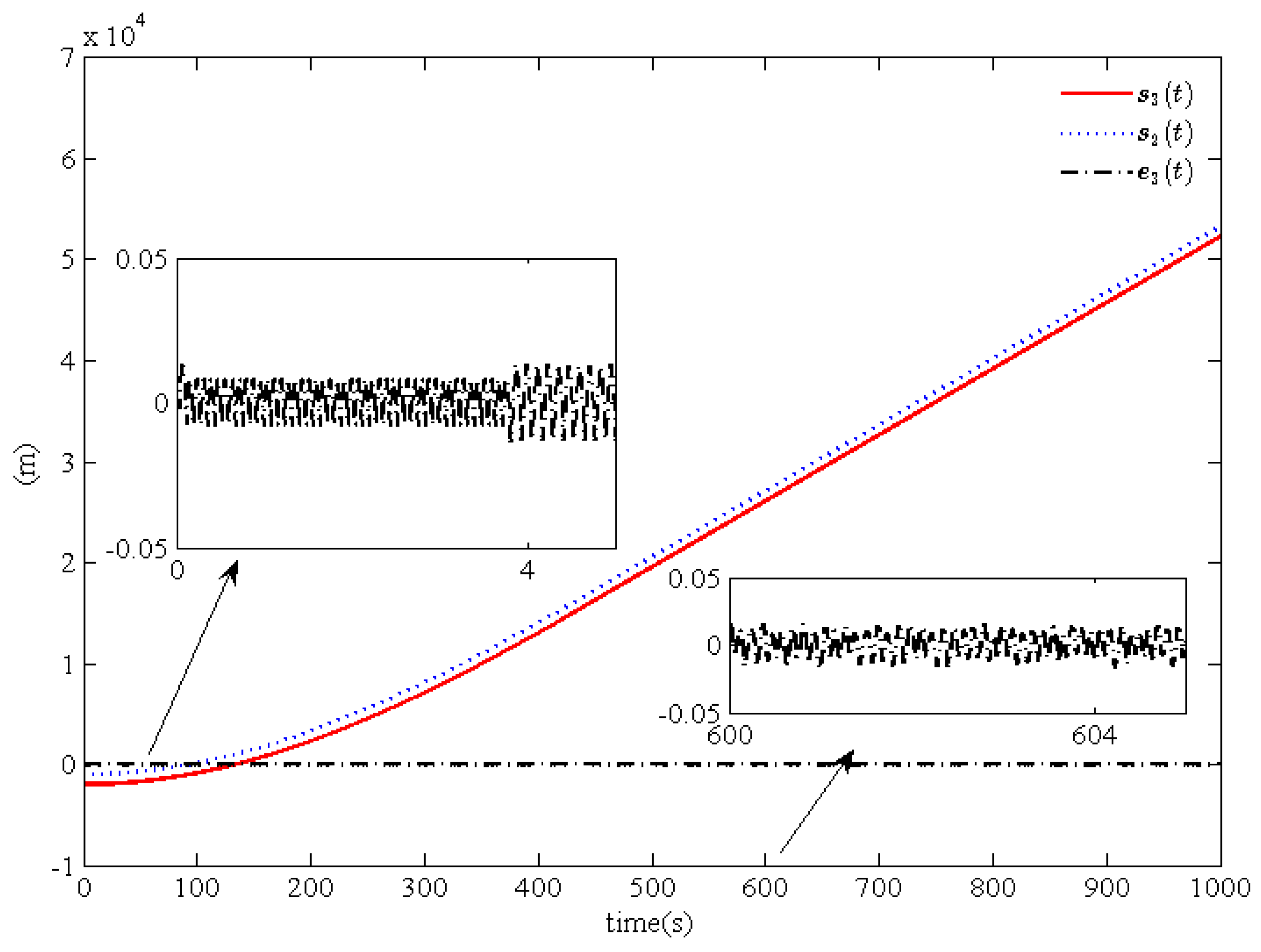
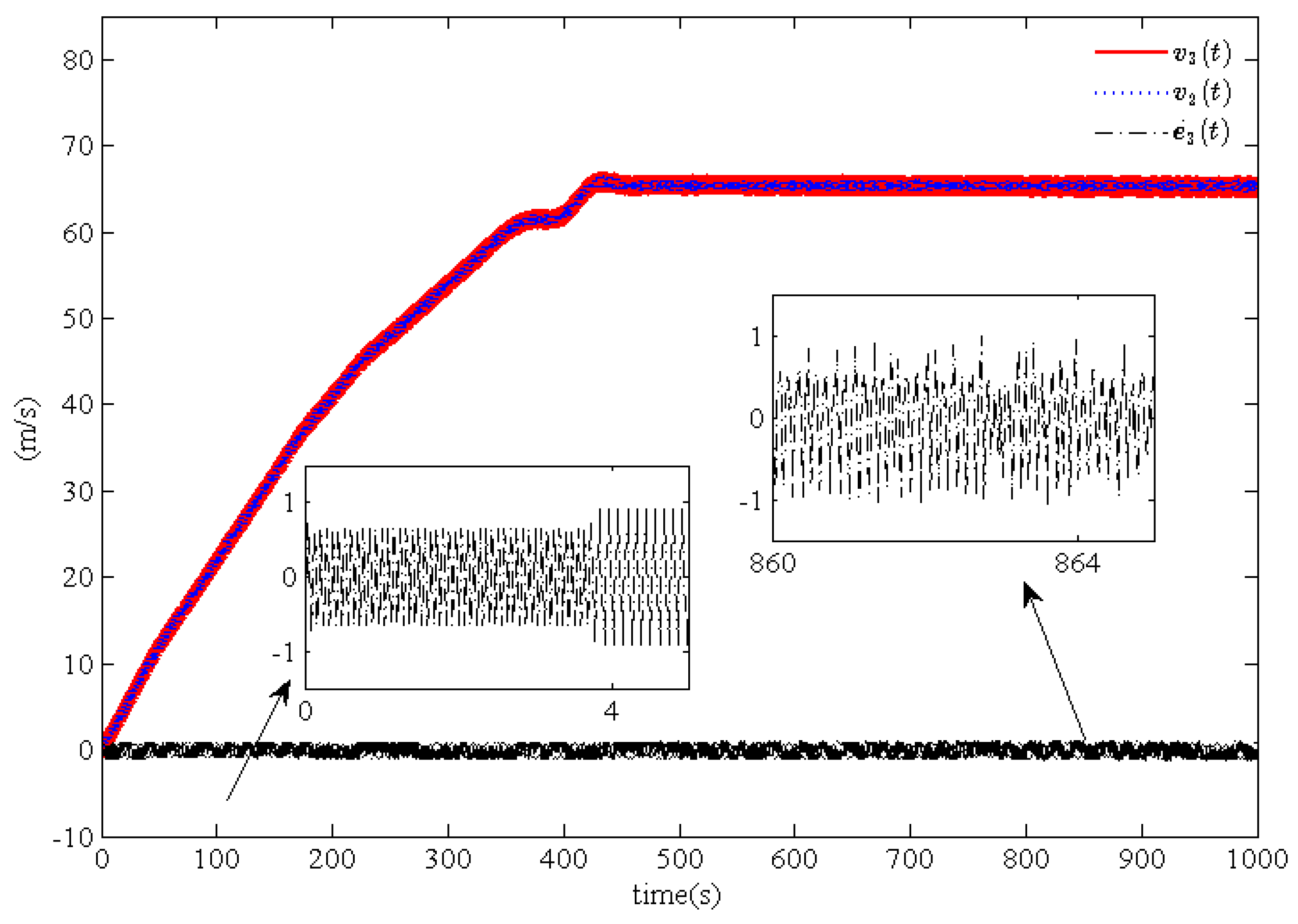
Figure 3,
Figure 5, and
Figure 7 show the actual position curves
, the desired position curves
, and the position tracking error curves
for trains
. Because of the chattering phenomenon resulting from the sign function, Equation (
7) is replaced with the following conditions in the simulation process:
where
if
,
if
, and ∗ denotes the function
or the function
.
Remark 10. To reduce the effects of the chattering phenomenon resulting from the sign function, we replace the saturation functions with it by means of [24]. According to
Figure 2, we can find that the position tracking error
of train
converges asymptotically to a small neighborhood near zero, which implies that a good desired position can be ensured for the leading train
. Similarly, good tracking performance for train
can be obtained. By comparing
Figure 2,
Figure 4, and
Figure 6, we can draw a conclusion that good position tracking performance for trains
can be obtained and that the convergence performance for train
is better than for trains
. According to
Figure 4 and
Figure 6, we can guarantee a safe disturbance
between the adjacent trains. At the same time, from
Figure 3,
Figure 5 and
Figure 7 we can draw the conclusion that the tracking performance of train
is better than train
or train
, which results from the convergence domain. In addition, the velocity tracking errors
and
converge asymptotically in a very small neighborhood near zero.
Based on the above analysis, by comparing the position tracking errors
,
,
and the velocity tracking errors
,
,
we can draw the conclusion that the tracking and cooperation performance for trains
are better than for train
. Meanwhile, it is obvious that the position tracking errors
,
,
and velocity tracking errors
,
,
asymptotically converge to a very small neighborhood near zero, which is matched by the presence of the leakage terms. Moreover, through a comparison of
Figure 2,
Figure 3,
Figure 4,
Figure 5,
Figure 6 and
Figure 7, it can be seen that the proposed cooperation control scheme is feasible and effective and that the desired tracking and cooperation performance can be obtained for multiple high-speed trains.

