Abstract
In this paper, the environmental uncertainties are taken into account when designing a robotic manipulator to balance the shaking force, shaking moment, and torque. The proposed robust balancing design approach does not consider the probability distributions of the uncertainties and is addressed without dependence on specific trajectories. This is expressed as a nonlinear constrained multiobjective optimization problem in which the nominal performance in the time-independent terms of the shaking force balancing, the shaking moment balancing, and the torque delivery, as well as their three sensitivities to uncertainties, are simultaneously optimized to provide a set of link shapes that match link mass distributions in a single stage. The proposal is applied to a three-degree-of-freedom serial-parallel manipulator, and the Non-Dominated Sorting Genetic Algorithm II (NSGA-II) is used to solve the associated problem. Comparative results with other design approaches reveal that the selected design achieves a suitable tradeoff in balancing the shaking force balancing, the shaking moment balancing, and the torque delivery and their sensitivities, leading to a reduction in their values and variations under mass changes in the manipulator end-effector with different operating conditions (tasks).
MSC:
74P10; 74G15; 90C56; 90C29
1. Introduction
Robotic manipulators create forces and moments related to the change in position in the mass centers of its components when the application is performed. These generated forces and moments can yield undesired movements in the task (inaccuracies and vibrations), resulting in a loss of precision and the necessity of significant support to keep the manipulator fixed to the base. Furthermore, these cause deterioration in the robot (wear and fatigue), reducing the lifetime and leading to sudden failures, which result in pausing the production (a one-day halt due to failure may cost up to EUR 100,000 or 200,000 [1]). In addition, the equilibrium between these forces and moments may significantly influence energy consumption. Finally, all these issues restrict the manipulator’s functionality in terms of speed, workspace, and application.
The energy exchange must be studied to obtain robotic manipulators (mechanisms) that perform the appropriate tasks with the minimum generation of undesired forces and moments. When the application speed is low, designers can only balance the gravitational and elastic energies by performing a static balance (gravity compensation) [2,3] or reducing the shaking force balancing [4]. High-speed manipulators are more likely to exhibit undesirable disturbances due to shaking moments [5]. Dynamic balancing, or the balancing of forces and moments, is a way to reduce or eliminate the harmful effects of high-speed mechanisms. In mechanical engineering, balancing mechanisms constitute an important topic that focuses on reducing these forces.
From the studies of Berkof in 1968 [6,7,8,9], several researchers have proposed different approaches to balancing the shaking force and the shaking moment in mechanisms. The importance of studying equilibrium in such forces and moments (reactionless conditions) in the robotic field began with the work in [10]. The main objective of dynamic balancing is to promote a synergy in the shaking force balancing and the shaking moment balancing, thereby reducing, as much as possible, the dynamic reactions at the base of the manipulator (mechanism or machine) caused by the structure’s motion [11,12]. The design tradeoff between shaking force balancing and shaking moment balancing is a challenging but important goal [13] since the first can affect the quality of the second and vice versa [14,15].
The dynamic balancing has been tackled by adding counter-mass systems to minimize the shaking force and including counter-rotating systems to reduce the shaking moment [5,9,16,17,18,19,20,21,22,23]. The counterweight systems can also include an equimomental system of point masses for creating a mass redistribution method [24,25]. These counterweight systems move the mass center of the whole system (robot). Similarly, auxiliary or duplicated mechanisms in a mirror manner have been added to the robot in order to perform dynamic balancing and thus counteract such forces and moments [13,26,27]. Other works also include a proper choice of trajectories for moment balancing with the use of an auxiliary mechanism to promote force balancing [28,29]. In [30], a pantograph mechanism is dynamically balanced in two sequential steps. First, the balancing conditions for keeping the linear momentum constant are found by using complementary components. Later, the force balancing conditions are determined by using Fisher’s method. Similarly, in [26,31], dynamic balancing is given by using specific trajectories, passive joints, and Fisher’s method. Other works include four-bar mechanisms in the development of the balancing of planar and spatial parallel robots [32,33,34]. Nevertheless, counterweight systems and auxiliary mechanisms add more mass to balance the mechanism. This results in a heavier mechanism that consumes more energy and incorporates more complexity into the kinematics and dynamics of the system (robot). Other alternative approaches have addressed the instantaneous balancing conditions for planar and spatial mechanisms by using the screw-theory-based methodology in the necessary instantaneous dynamic balancing conditions [23]. The use of higher-order derivatives of the balance conditions [35] is another approach that could result in easier and less expensive methods for the dynamic balancing of a small group of closed-loop linkages. Anther approach to fulfilling the necessary conditions for the complete shaking force and shaking moment is using the equivalence method [36], where complex planar mechanisms are transformed into simple equivalent links and cranks as the equivalence method [36]. On the other hand, fulfilling the dynamic balancing conditions assumes strict constraints on the dimensional parameters of linkages or sets very restrictive conditions that are sometimes difficult to achieve in practice.
On the other hand, optimization approaches have been incorporated in the balancing of mechanisms. In [37], both a counterweight system and a spring are simultaneously designed to minimize the reaction forces of a planar five-bar parallel robot subject to the static balancing conditions (equations that fulfill constant potential energy), and the limits in the design variable vector. Matlab’s Sequential Quadratic Programming (SQP) is used to solve the problem. In this case, the minimization of the shaking force produces a lighter robot than those designed using only counterweight systems (without springs). However, this approach does not consider shaking moment conditions. A reactionless, two-degree-of-freedom, planar parallel mechanism is designed in [38] to reduce mass and inertia by optimizing a counter-mechanism to moment balance a force-balanced mechanism. The force balancing conditions and the dynamic balancing conditions are set as constraints. The Lagrange multipliers are used to solve the optimization problem. In [39], the location and orientation of the task to be performed by an orthoglide parallel robot are optimized according to the shaking force changes, the shaking force maximum value, the maximum actuator torques, and the energy consumption subject to the geometric, kinematic, and dynamic constraints. A multiobjective optimization problem is proposed and solved by using the Multiobjective Genetic Algorithm (MOGA), where the obtained design solutions depend on the trajectory to be performed by the robot. In [40], a reduced number of equivalent dynamic parameters of a set of three point-masses dynamically equivalent to the dynamic parameters of rigid links of a mechanism are designed for balancing the shaking force and shaking moment subject to the limits of the equivalent dynamic parameters (equimomental system [41,42]). The approach is stated as a mono-objective optimization problem tackled as a weighted sum approach. The Genetic Algorithm (GA) of Matlab is used to solve it. As the solution to this problem does not provide the shape of the link, another optimization problem is proposed to match the optimal link mass distribution. For this purpose, the dynamic parameters of the link are obtained from a link shape parameterized through cubic B-splines. Then, the second optimization problem consists of finding the Cartesian coordinates of the links formed by B-spline curves that minimize the error of the link inertia subject to the fulfillment of the other link dynamic parameters (mass and Cartesian mass center position). Matlab’s GA is also used to solve the second optimization problem. This two-stage optimization approach can lead to the degradation of the dynamic balancing due to the error detected between the link shape and the equivalent dynamic parameters. In [43], the forces, torques, and shaking moment sensitivity with respect to position, velocity, and acceleration changes are selected as a weighted performance function in the optimization problem. The constraints are related to the fulfillment of the shaking force balancing requirements. This approach is applied to a two-degree-of-freedom parallel manipulator to follow a cycloidal motion. The obtained design is achieved by SQP, concluding that the shaking moment sensitivities can also reduce the shaking moment. In [44], to fully balance the force of the mechanism while minimizing the shaking moment, the counterweight approach and the adjusting kinematic parameters [45,46] are integrated to provide a unified strategy for partial moment balancing. This is applied to a spherical parallel robot. The AKP technique is used to change the length of the links with the CW method to discover the extra masses and their positions, to minimize the shaking moment while still meeting the requirements of force balancing. The problem is solved by using the SQP algorithm of Matlab. The main drawback of the approach is the requirement of some kinematic relations to fulfill the balancing conditions, which may be difficult to satisfy. In [47], the time-independent terms of the shaking moment and shaking force are simultaneously optimized by using a weighted sum approach to suggest a balancing design for various operating conditions (tasks). This results in a unified design approach for the mass distribution scheme and the link shape. Nevertheless, the a priori selected tradeoffs based on the objective performance weights require precise knowledge of the importance of each objective and a process called normalization to scale different orders of magnitude in the objectives. Unfortunately, these requirements are not easy to fulfill because, in the former case, a set of uniformly distributed weights does not result in a set of Pareto solutions that are also uniformly distributed, which makes it challenging to set weights in order to achieve a Pareto solution in a desired area of the objective space. Moreover, in the second case, the normalization must be performed by solving several single-objective optimization problems, one for each objective function. This is a very time-consuming task. In addition, the weighted sum approach has problems in non-convex Pareto fronts (it cannot find solutions in this type of front).
Through the reviewed literature, it is observed that both deterministic and stochastic algorithms have been used to explore the design space of the balancing problem. Within deterministic algorithms, gradient-based ones [48] might become stuck in local solutions, while convex optimization [49] requires extensive mathematical analysis to transform a multimodal optimization problem into a convex optimization one. In recent years, evolutionary algorithms (a type of stochastic algorithm inspired by natural evolution) have been used to solve the balancing problem due to their insensitivity to the initial condition that tends to leave local regions, their practical implementation (simple and effective) in a variety of optimization problem domains, and their ability to combine different operators into the search. Algorithms based on Genetic Algorithm (GA) [40,50,51,52] and Differential Evolution (DE) [53] are the most commonly used in the reviewed literature.
1.1. Contributions
The approaches to dynamic balancing have been laid out for a specific kinematic structure or a family of mechanisms, where it may be challenging to identify design solutions to maintain balancing in a mechanism that has not been discussed in the literature. Moreover, the requirement of assumptions such as having a smaller design space in the optimization problem due to the requirement of certain operational conditions (trajectories), the inclusion of auxiliary devices (mechanisms, counterweights, or transmissions), and the setting of strict constraints on the link parameters could reduce the effectiveness of dynamic balancing, and the use of a constant load limit the search for potential design solutions. These issues restrict the benefits that may be achievable.
Recently, the need to provide a dynamic balancing solution for general-purpose applications in manipulators in a single design step has led to the search for other multitask dynamic balancing approaches that take into account the tradeoff between shaking force balancing and shaking moment balancing. Nevertheless, to the best of the authors’ knowledge, this issue is only addressed in [47].
In addition to adopting a balancing approach for multipurpose applications as in [47], the varied load management in the robot’s end-effector is a significant factor in manipulator tasks, which, to the authors’ knowledge, is not addressed in the state-of-the-art. Clearly, managing different loads can deteriorate the balance of the shaking force, shaking moment, and torque delivery. In order to reduce the impacts of load fluctuations on the shaking force, shaking moment, and torque delivery, a robust balancing strategy for robotic manipulators is proposed in this paper. This is the first contribution of the paper.
The proposed robust balancing approach is based on optimization in which the shaking force balancing, shaking moment balancing, and torque delivery of the obtained design are as insensitive as possible to uncertainties in the environment (such as the load) and are also independent of the operating conditions (such as different tasks). This is formulated as a constrained multiobjective optimization problem in which the sensitivity of the time-independent parameters of the shaking force, the shaking momentum, the torque, and their nominal values are all optimized at the same time to provide a set of design tradeoffs. One benefit of the proposal is that the optimization process does not need to know the uncertainty variations (the probability distributions of the variations). Instead, it only needs to know the nominal values of these variations. As a result, the obtained design solutions provide the most competitive performance function tradeoffs for various end-effector loads and trajectories. In this framework, it is also possible to find a set of Pareto solutions in a single algorithm execution, and the decision maker for a single tradeoff is chosen from the design solutions found.
The Non-Dominated Sorting Genetic Algorithm-II (NSGA-II) [54] is used to solve the constrained multiobjective optimization problem formulated in the proposal. The proposal’s efficacy is applied to a three-degree-of-freedom planar manipulator where both the shape and the optimal mass distribution of links are designed to fulfill designs with less sensitivity in the shaking force, the shaking momentum, and the torque under load variations. Thus, the effectiveness of the proposal is empirically validated. This last result represents the last contribution of the work.
1.2. Paper Organization
The remainder of the paper is structured as follows: Section 2 states the robust balancing problem. The practical application (case study), its associated multiobjective optimization problem, and the evolutionary optimization technique to solve it are presented in Section 3. The results and discussion are given in Section 4, and, finally, the conclusions are drawn in Section 5.
2. Design Approach Based on Multiobjective Optimization for Shaking Force, Shaking Moment, and Torque Robust Balancing
The proposed design approach consists of the robust balancing of the shaking force, the shaking moment, and the torque of robotic manipulators, assuming that there are uncertainties that are not modeled in the proposal. The proposed robust approach for balancing robotic manipulators is stated as a nonlinear constrained multiobjective optimization problem (NLC-MOP). The solutions provide a set of tradeoffs that perform different synergies among the design criteria and reduce their variations in the presence of uncertainties, i.e., the shaking force, the shaking moment, and the torque are as insensitive as possible to such changes.
The application of the robust balancing approach requires the following simplifying assumptions:
- (1)
- The i-th objective function (design criterion) ∀ must be of at least class for developing the design objective variations .
- (2)
- The nominal value of the uncertainty parameter is known, but its variations and bounds are not (probability distributions of the variations are not known).
- (3)
- The design criteria related to the shaking force, the shaking moment, and the torque can be divided into time-dependent and time-independent terms.
In addition, the non-robust balancing approach given in [47] is considered to be generally stated as follows:
subject to
The problem formulation (1)–(4) is related to a multiobjective optimization problem that has been transformed into a single-objective optimization one by using the weighted sum approach [55], where term represents the i-th design objective weight. It includes design criteria (each one in , ) that are weighted in J and inequality constraints (3) inherent to the balancing problem. The design criteria are related to the time-independent terms of the shaking force, shaking moment, and torque to make the design not dependent on the operating conditions (performed trajectories) of the robot [47]. The design parameters allow the distribution of the link masses to fulfill the design objective and constraints. These parameters are related to the link shape and grouped in the vector with the lower and upper limits and , respectively. In contrast to [47], the formulation includes the uncertain parameter vector . The uncertain parameter differs from its nominal value by units and is associated with parameters that can change depending on the application. In the case reported in [47], the uncertain parameter vector is not considered (it does not appear in the optimization problem), and this vector is assumed to be at its nominal value, i.e., . Nonetheless, the uncertainties can deteriorate the optimal solution in the balancing problem such that the performance function can be negatively affected, or even the solution can leave the feasible region. For this reason, the formulation of a robust balancing approach is proposed in this work.
The robust balancing approach is formulated as a multiobjective optimization problem where the nominal design objectives and their variations with respect to unknown changes are considered objective functions. The nominal objectives involve the terms in (2) associated with the design objectives of the non-robust balancing approach. In the proposed formulation, the uncertainties present a known nominal value but their variations are not known. The previous assumption is common in several applications. For example, considering friction as uncertainty, the friction of the robot joint can increase with the operating time and the environment, among others, and, for this case, the designer knows the initial joint friction (nominal value) and does not know the friction when time goes by (variation value). Thus, the design objective variations refer to the rate of change in the terms with respect to the uncertainty variations (which are assumed to be infinitesimal) considering the nominal value of uncertainties . The i-th design objective variation with respect to the j-th uncertainty (sensitivity) can be expressed as in (5).
Therefore, the general formulation of the robust balancing approach is stated as the multiobjective optimization problem in (6)–(8). It consists of finding the set of link shapes grouped in the design variable vector that satisfy different tradeoffs among the nominal design criteria related to the shaking force, shaking moment, and torque, as well as variations in these criteria subject to inherited constraints in the balancing problem.
subject to
It is important to point out in the proposal whether (5) is decreased, the changes in the design objectives due to variations in the uncertainties are reduced, and, then, the minimization of can provide solutions as insensible as possible to uncertainty variations in the design objectives . Moreover, the minimization of the nominal design objectives can provide solutions with better performance. Then, when the robust balancing problem formulation is solved, the proposal can search for different solutions that fulfill different tradeoffs in minimizing the nominal performance functions and their variations due to the multiobjective nature of the problem formulation. Section 3 gives the details of the optimization problem for the robust balancing approach in a specific application.
Multiobjective Optimization Algorithm
The Non-Dominated Sorting Genetic Algorithm II (NSGA-II) [54] is implemented to solve the robust balancing optimization problem (6)–(8). The NSGA-II is chosen because it can identify a better distribution of solutions and convergence around the true Pareto-optimal front in benchmark optimization problems. Furthermore, as mentioned in the Introduction, GA-based algorithms are more commonly utilized to solve balancing problems.
The pseudocode of the NSGA-II is shown in Algorithm 1. Considering constrained multiobjective optimization problems, the NSGA-II starts with a random parent population sorted based on the non-domination level (using constrained domination). Similar to the GA algorithm, it uses binary tournament selection, recombination, and mutation operators to create the offspring population from the parent population. Both populations are combined and sorted according to the non-domination level. The new parent population is formed by selecting the solutions from the best domination levels until this population is filled. The crowded-comparison operator (based on non-domination level and crowding distance) is used to prune the solutions in the last front of the combined population. The same procedure is done (recombination and mutation) in the new parent population, but now the selection criterion in the binary tournament selection is based on the crowded-comparison operator. This process is repeated until the desired generation is reached.
In the implementation, the simulated binary crossover (SBX) operator and polynomial mutation are used as in the original work [54]. Nevertheless, the technique to handle bound constraints in the generation of the offspring population is changed to the random bound constraint-handling method [56]. This method substitutes random values for variables outside the bounds.
On the other hand, the search space for the robust balancing problem is complicated because there are many design variables, many constraints, and many performance functions that need to be optimized. Thus, an elite solution (promising solution) is added to the random parent population to be used in the search for exploration and exploitation in the elite region. Furthermore, the entire region is explored and exploited, as described in the original work. The method of obtaining this elite solution and its parameters are detailed in Section 4.1.1.
With the aforementioned changes, the NSGA-II is used to find solutions to the robust balancing problem.
| Algorithm 1 Pseudocode of the NSGA-II. |
|
| Algorithm 2 Simulated Binary Crossover (SBX). |
|
| Algorithm 3 Polynomial mutation. |
|
3. Application
The proposed robust balancing problem is applied to a hybrid serial-parallel robotic manipulator. In the proposed approach, the dynamic balancing conditions, the torque, and their variations are simultaneously considered to provide a suitable mass distribution of the manipulator links that keeps robust solutions. In what follows, the robotic manipulator, as well as the terms associated with the optimization problem (6)–(8) of the proposal, are presented.
3.1. Robot Description
The schematic diagram of the considered robotic manipulator is shown in Figure 1. This robot presents a hybrid architecture based on a parallel and serial structure with three degrees of freedom ( ) in the joint space. It develops the task in the plane considering the Cartesian position (, ) and orientation of the end-effector. The angular position and velocity of links are expressed as and , respectively; the input torque vector is given by and the gravity acceleration is set as g.
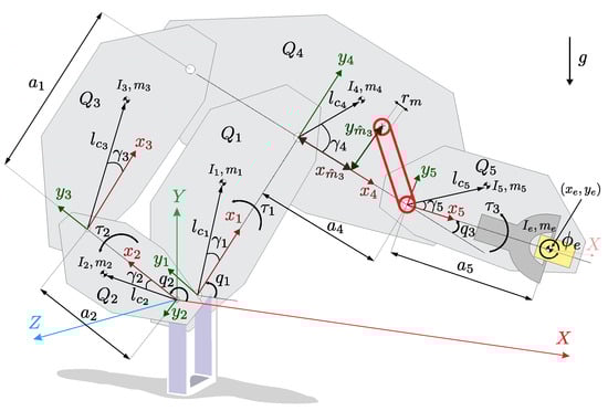
Figure 1.
Schematic diagram of the robotic manipulator.
3.2. Design Variables
Before setting the design variables, it is important to note that each link has its own coordinate system to describe the position of the link mass center at the origin of such a system, through the polar coordinates (see Figure 1). Given the polar coordinates above, the Cartesian coordinates of each link can be calculated as and . On the contrary, given the Cartesian coordinates of the link, the polar ones result in and .
Moreover, for each link, there is information about the inertia tensor , the mass , and the link lengths . The actuator of the fifth link with mass is located at the coordinate from the coordinate system (link ) with a 1:1 pulley and belt transmission. In general, the actuator has a relatively high weight. Unlike when the actuator of the fifth link is placed in a specific location, the mass distribution of the robot can be more precisely configured by moving the actuator’s weight to different locations.
The design parameters to fulfill the design objectives in the proposal are the link mass distribution considering constant link lengths. Each link mass distribution is modified according to the independent geometric variables of octagonal link shapes (, , , , , , , , , ). In the case of the link , the position of the motor that provides the movement in the link is also adjusted as observed in Figure 2 because it can influence its mass distribution. Then, the design variable vector can be grouped and presented in (9).
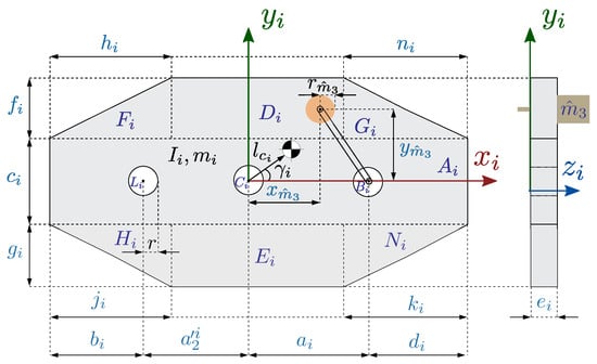
Figure 2.
Design variables of the i-th link. The distance of the fourth link () is set as a fixed length and the cylinder (hole) is included. For the rest of the links (∀), the fixed length , the cylinder , and the actuator placed in are removed (the length, the hole, and the actuator are not considered).
The octagonal link shape is a proposal given in [47] to promote different configurations of the link to change its mass, inertia, and mass center length, i.e., with different values of its independent geometric variables, the links can form rectangular, trapezoidal, hexagonal, octagonal prisms, or irregular forms. The main advantage is that the increment in the link mass and system complexity in the mass redistribution by using the link shape is less likely as in the case of the counterweight approach [25], because it is necessary to add counterweight systems to fulfill a specific mass redistribution in a given link. Meanwhile, the links are designed from scratch using the link shape for mass redistribution.
The relationships between the mass , the inertia , and the mass center length of the robot links with respect to the design variable vector are then depicted next [47].
Considering that the mass, the mass center position, and the inertia of the i-th link can be formed from simple geometries, (see Figure 2). The mass, the mass center position, and the inertia of the i-th link can be expressed as a function of as expressed in (10)–(13).
In addition, each simple geometry in has a mass , a mass center length expressed in Cartesian coordinates (with respect to the coordinate system ), and an inertia moment in the z axis, and these are expressed in Appendix A.
3.3. Nominal Performance Function
In this section, the performance functions related to the shaking force, shaking moment, and torque are detailed. In all design objectives, the time-dependent terms are removed to promote design objectives free of specific applications.
3.3.1. Shaking Force
The robotic manipulator’s total mass center vector multiplied by the manipulator total mass can be expressed as in (14), where and are the mass and mass center position of the i-th link, respectively.
Then, the shaking force vector (15) can be formulated using the second derivative of (14), where and are the linear acceleration of the i-th link mass center and the total mass center vector, respectively.
When the Global Center of Mass (G.C.M.) of a robot remains constant regardless of the motion of the manipulator, the total force applied by the robot to the fixed base remains constant as well [57]. In this case, the forces acting on the manipulator frames should ideally add up to zero, and the shaking (force) balancing condition is satisfied [7].
By using complex numbers and the Euler identity to represent a two-dimensional vector to a complex number, and separating the time-dependent vector related to the generalized coordinates , the mass Equation (14) results in (16) [47].
Let us consider that the real and imaginary part of the time-independent complex number in (16) is grouped in the matrix where , , , , and . The Frobenius norm of the matrix (18) is chosen as the design objective to reduce the time-independent terms of the shaking force balancing (17). Minimizing this objective function will reduce the shaking force balancing.
It is important to note that the objective function (18) represents the square of the terms and it does not depend on a specific application (i.e., it does not depend on , and ).
3.3.2. Shaking Moment
According to [47], let us consider that the angular momentum (19) in the z axis can be expressed in the time-independent and time-dependent vectors named as and , respectively.
where , , represent the mass center velocity vector, the angular velocity vector, and the inertia tensor of the i-th link. is a unit vector in the z direction. The terms of the vectors and are , , , , , , , , , , , , , , , , , and .
Assuming that the mass, mass center length, inertia, and length of links do not vary with respect to time, the shaking moment in the z axis is expressed in (20).
3.3.3. Torque Delivery
Since the joint actuator provides the applied torque to fulfill the task, i.e., the motor torque must compensate the load (due to the manipulator dynamics with its end-effector load) for governing it ( ), minimizing the manipulator load can reduce the applied torque and thus the energy consumption.
Then, the closed-form dynamic model derived from the Lagrange equations [58] is (22), where ∈ is the symmetric and positive, definite inertia matrix; ∈ is a matrix that relates the centrifugal and Coriolis forces when multiplied by the angular velocity , and ∈ is the vector of gravity. Appendix B provides information about the terms included in the matrices and vectors of the dynamic model.
Considering that the robot dynamics (22) are linear in the inertia parameters [58], the robotic dynamics can be expressed as the product of a time-dependent matrix (referred to as the regressor), and a vector called the inertia parameters (constant vector). With the linearity property in the inertia parameters of the robotic manipulator dynamics, there can also exist matrices and ∀, which contain the time-dependent terms (the state vector), and also a matrix that contains the inertia parameters of the robot. In these matrices, and represent the number of columns or rows in such matrices. For instance, the matrix when results in .
Hence, it is possible to rewrite the matrices and and the vector as in (23), (24), and (25), respectively. See Appendix C for the details of these matrices.
The squares of the Frobenius norms of the matrices , , and are proposed as the other design objective (26). The minimization of such time-independent terms (design objective) can reduce the applied torque (22) exerted by the robotic manipulator without a dependency on a specific robotic application, i.e, without relying on the generalized coordinates , velocities , and accelerations .
3.4. Variations in the Performance Function (Sensitivities)
This section explains the performance function related to the decrement in the variation in the nominal objective function with respect to uncertainties. As commented previously, these objectives are expressed without dependence on time to promote design objectives free of specific applications.
In this case, the end-effector load applied in the Cartesian coordinate of the fifth link (see Figure 1) is considered as the parameter that changes in different applications of the robot manipulator. Then, the mass of the fifth link is chosen as the uncertain parameter () due to the changes in the end-effector load directly modifying the corresponding link’s mass distribution.
It is important to note that the first through third objective functions (18), (21), and (26) depend on , , , , i.e., these are composite functions ∀. Their variations are computed by differentiating composite functions.
3.4.1. Shaking Force Variation
The variation in the Time-Independent Terms of the Shaking Force Balancing (TITShFB) (18) with respect to the fifth mass is named . The square of (27) is selected as another objective function to be minimized. Minimizing this objective function will promote robust solutions for the TITShFB and, therefore, it reduces the shaking force balancing variations.
Therefore, the objective function related to the TITShFB (27) is expressed in (37).
3.4.2. Shaking Moment Variation
The variation in the Time-Independent Terms of the Shaking Moment Balancing (TITShMB) (21) with respect to the fifth mass is named . The square of (38) is selected as another objective function to be minimized. Minimizing this objective function will promote robust solutions for the TITShMB and, therefore, it reduces the shaking moment balancing variations
The term can be obtained as follows:
where
Substituting (33)–(36) and (40)–(43) in (39) and squaring this term, the objective function related to the variation in the TITShMB (38) can be obtained, but this is not explicitly expressed due to the large expression of this function.
3.4.3. Torque Variation
As commented previously, the torque delivery is related in this work to the Time-Independent Terms of the Applied Torque (TITAT). Then, the variation in the TITAT (26) with respect to the fifth mass is named . The square of (44) is selected as another objective function to be minimized. Minimizing this objective function will promote robust solutions for the TITAT and, therefore, it reduces the torque variations
The term can be obtained as follows:
where
Substituting (33)–(36) and (46)–(49) in (45) and squaring this term, the objective function related to the TITAT (44) can be obtained, but this is not explicitly expressed due to the large expression of this function.
3.5. Design Constraints
The design approach requires that the link shapes form prisms and the location of the third motor is also placed inside the fourth link [47].
The link shape requirements are related to the following twenty constraints (50)–(53), where and are the maximum allowed height and width, respectively.
The motor position requirements involve the following nine constraints (54)–(62), which restrict the mass center of the motor to be outside the green area of the fourth link, as is observed in Figure 3. In these equations, is the tolerance radius and is the minimum distance from the motor coordinates to the diagonal lines .
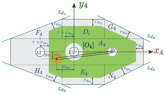
Figure 3.
Graphical representation of the allowed area for placing the motor in the fourth link.
The last constraints involve the bounds of the design variable vector stated in (63) and (64).
For a detailed description of the above constraints and the design variable limits and , consult [47].
3.6. Statement of the Robust Balancing Optimization Problem
The robust balancing of the shaking force, shaking moment, and torque is formulated as a constrained nonlinear multiobjective optimization problem. This consists of finding the link shapes and the motor placement that fulfill a set of tradeoffs for balancing the shaking force, shaking moment, and torque, as well as their variations under the effects of mass changes in the end-effector of a hybrid robotic manipulator. The design variables are also constrained by the link shape, the motor location, and their limits. The formal and general description of the optimization problem is set in (65) and (66).
subject to
4. Results
This section is divided into two parts to analyze the obtained design with the proposed robust balancing. The first part of this section establishes the conditions for optimizing the robust balancing problem. Subsequently, the resulting Pareto front is presented. Afterward, the decision making is detailed, and the selected solution is analyzed and discussed. Finally, in the second part, the selected design is compared with other design approaches to discuss the advantages of the proposed robust balancing.
4.1. Optimization Process
4.1.1. Experiment Conditions
The NSGA-II solves the optimization problem with a population size of 200 chromosomes and a maximum number of 100,000 generations. The algorithm parameters are chosen according to Table 1 and they are set empirically. The constant optimization problem parameters are also shown in Table 1 and the limits of the design variable vector in Table 2. The structural material of the links is chosen in the optimization process, and the material density is constant. Aluminum is used for the link design in the study case. Ten independent executions are performed, and all obtained Pareto solutions are filtered by the crowded-comparison operator [54] to set a single Pareto front among all executions.

Table 1.
Parameters of the NSGA-II and the optimization problem.
Table 2.
Boundaries of the design variable vector.
The difficulty of the proposed balancing problem is finding a useful tradeoff to handle the six performance functions. This leads to the inclusion of a promising individual (elite solution) in the NSGA-II’s initial population to promote the search in this region as well as other random regions. The selected promising individual is obtained from [47]. The elite solution is the design that comes from solving the dynamic balancing design in [47] using the differential evolution algorithm, while taking into account both the shaking force and shaking moment. The design variable vector of the selected promising individual is presented in Table 3.
Table 3.
The design variable vector (elite solution) included in the initial population.
The experiments described in the following section are performed on a personal computer equipped with an Intel(R) Core(TM) i5-63000 CPU running at 2.4 GHz and 16 GB of RAM. The NSGA-II is programmed using Matlab. The convergence time of the ten independent executions is h.
4.1.2. Pareto Front
The Pareto front obtained by filtering the ten independent executions is presented in two-dimensional spaces in Figure 4, Figure 5 and Figure 6. In total, 1023 Pareto solutions are obtained. In the figure, the solutions of other design approaches reported in [47] are displayed, and these designs are compared with the obtained robust balancing design in the next section. These solutions include the Dynamic Balancing Design (DBD), where the time-independent terms of the shaking force balancing and the shaking moment balancing are simultaneously optimized by stating a weighted sum mono-objective optimization approach. The other solution is related to a Shaking Force Balancing Design (SFBD) where the main performance function is the time-independent term of the shaking force, and the last solution is a Shaking Moment Balancing Design (SMBD) that only minimizes the time-independent terms of the shaking moment. One more solution is introduced in the Pareto front of Figure 4, Figure 5 and Figure 6. This solution is obtained by optimizing the nominal performance functions by a multiobjective optimization approach without considering its variation, i.e., the optimization problem is related to the minimization of the objective function vector given by the time-independent terms of the shaking force balancing, the shaking moment balancing, and the torque. The obtained solution is named Dynamic and Torque Balancing Design (DTBD). It is important to point out that the RBD, DBD, and DTBD stay in the same region of the Pareto front from Figure 4, Figure 5 and Figure 6, whereas SMBD and SFBD present different performance. The latter is confirmed in Figure 7, where the radar plot is given for the six design approaches, and similarities between the DBD and the DTBD arise. On the other hand, the two-dimensional space of the Pareto front suggests a strong correlation between two performance functions (see, for instance, in Figure 4b), and then the possibility of reducing the problem dimension. Nevertheless, other non-reported experiments in this paper were developed where only two performance functions (for instance, and ) are considered in a new bi-objective optimization problem with the same design variables and constraints stated before. The obtained solutions indicate that the dimensionality of the optimization problem cannot be reduced because of the existence of tradeoffs between performance functions.
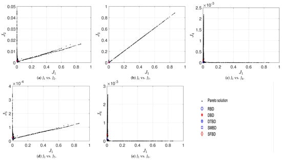
Figure 4.
Pareto front in two-dimensional spaces (1/3).
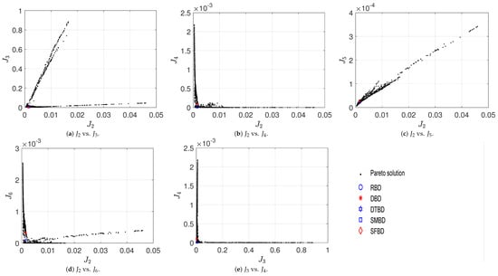
Figure 5.
Pareto front in two-dimensional spaces (2/3).
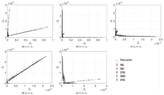
Figure 6.
Pareto front in two-dimensional spaces (3/3).
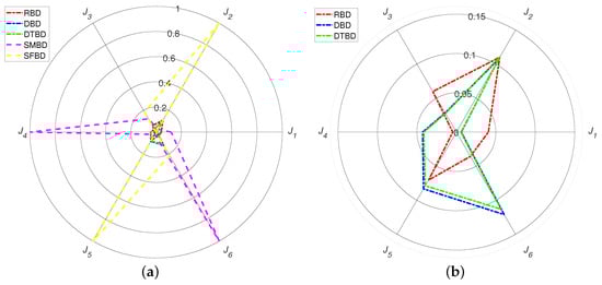
Figure 7.
Performance functions of the design approaches. (a) Radar plot. (b) Close-up view.
4.1.3. Decision Maker
The decision making among all Pareto solutions (1023 Pareto solutions) shown in Figure 4, Figure 5 and Figure 6 is a challenging task. The following steps are used to choose a competitive robust balancing design (RBD).
First, the Pareto solutions that improve the norm of the performance variations (given by the objective functions ) of the selected promising solution (DBD solution included in the initial population of the optimization process) are only considered.
Once these solutions are grouped, the second stage consists of selecting, from this group, the solution that approximates the DBD solution in the first three objective functions (nominal objective functions) with and without variations in the dynamic parameters of the fifth link. In this stage, the variations in the nominal objective functions with respect to changes in the fifth link () mass, its mass center position, and inertia are considered. The modification of the fifth link is attributed to a possible load in the robot end-effector placed in in Figure 1, named its mass as and the inertia moment as . This load is given by a cylindrical disk that modifies both the fifth link mass as , the coordinate of the mass center length as , and the inertia as . Thus, the time-independent terms of the shaking force , shaking moment , and torque vary with respect to the mass .
Hence, twelve different disks (different and ) are incorporated into the robot end-effector (one at a time) of the obtained designs from the group. The corresponding nominal objective functions are compared with respect to that of a selected promising solution (DBD solution shown in Table 3, included in the initial population of the optimization process in the RBD). Then, the solution in the group that sums more wins in the nominal objective functions, considering different disks, is selected. At the end of the second stage, the decision making is done, and a single design solution of the robust balancing design approach is obtained. The design variable vector obtained from the RBD and the dynamic parameters of the links are shown in Table 4 and Table 5, respectively.
Table 4.
Design variable vector obtained from the robust balancing design (RBD) approach.
Table 5.
Dynamic parameters of the RBD.
The obtained robust balancing design (RBD) given in Table 4 is analyzed according to variations in the nominal objective functions with respect to twelve changes in the disk, as described above. The values of the objective functions of such comparisons are given in Table 6. It is observed in such a table that without a disk (), the DBD presents smaller values in the nominal objective functions (the three first objective functions), but it has more value in the last three objective functions. An increase in the last three objective functions indicates a growth in the sensitivity of the nominal objective functions. This increment implies that when the disk is added () in the DBD, the variation in the nominal objective functions is more affected by its magnification. In the case of RBD, this is less influenced by the disk parameters (, ) because it presents the smaller difference in the interval of the objective function variations (see columns) with respect to the DBD. As a consequence, the values of the nominal objective functions (see columns) present smaller values with respect to the DBD, concluding that the obtained solution with the RBD approach presents a reduction among , , in the time-independent terms of the shaking force balancing, shaking moment balancing, and torque, respectively.
Table 6.
Performance functions of the RBD and the DBD under the effect of mass variations.
4.2. Comparative Results with Other Design Approaches
This section compares the obtained robust balancing design with other design approaches. The approaches to be compared are the DBD, the DTBD, the SFBD, and the SMBD, which are detailed in Section 4.1.2. The main objective is to know the performance of the RBD in the shaking force balancing (15), the shaking moment balancing (20), and the torque (22) with different tasks (trajectories), execution times, and end-effector weights. In this case, the time-dependent and the time-independent terms of such functions are simultaneously considered in the analysis, i.e., the Root Mean Square (RMS) value of the resultant force vector in the shaking force balancing (), the RMS value of the shaking moment balancing in the axis (), and the RMS value of the torque () are examined.
The experiment consists of using four trajectories (hypocycloid, circle, lemniscate, and line) with three different execution times ( s, s, and s) and four variations in the end-effector load ( kg, kg, kg, and kg). A total of 60 numerical simulations are developed for each compared design. The dynamic parameters of the designs to be compared are presented in Table 7, and the Computer-Aided Designs (CADs) are shown in Figure 8. It is observed that the mass of the SMBD decreases its mass in , the DTBD in , the DBD in , and the SFBD increases its mass in with respect to the RBD. Thus, the RBD presents a suitable total mass ( kg) concerning state-of-the-art designs.
Table 7.
Dynamic parameters of the DBD, the DTBD, the SFBD, and the SMBD.

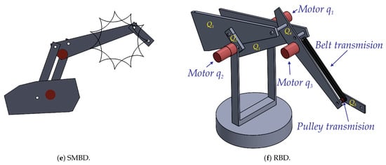
Figure 8.
CAD of the different design approaches. Lateral views of the obtained links (a–e). Isometric view (f) of the RBD with base.
Table 8, Table 9, Table 10 and Table 11 present the comparative results of the proposed RBD with respect to DBD, DTBD, SMBD, SFBD, respectively. The first column indicates the type of trajectory, the second one shows the applied mass to the end-effector, the third to fifth columns include the RMS values of the indicators stated above, and the last column sums the number of wins in the comparison for each indicator per row (the smallest value in the comparison wins). The values in boldface indicate an improvement with respect to the counterpart (the winner in the comparison). Furthermore, the shadowed rows “Mean variations” in Table 8, Table 9, Table 10 and Table 11 indicate the average of the difference between the RMS value of the indicators with two different masses in the end-effector. The computation of such rows is illustrated with a particular example. For the hypocycloid trajectory, the RMS value of the DBD in the third column (shaking force) of Table 8 presents a value of when the end-effector mass is kg. On the other hand, when this mass changes to kg, it produces a value of . Thus, the difference (variation) in the RMS value for this particular mass change is . Similarly, four different variations are computed in this example (, , , 1538), and the average of the variations in the shaking force RMS value for the DBD is set in the shadowed row, i.e., the value of . The same procedure is done for the next data to complete the three columns (from third to fifth). It is clear that the smallest value in the comparison of the mean variations indicates a reduction in the indicator’s sensitivity with respect to mass changes. Thus, more wins in the mean variations result in a design that is more robust under mass variations. The shaking force, shaking moment, and torque behavior for the five designs executing the four trajectories with the two different end-effector masses are shown in Figure 9, Figure 10, Figure 11 and Figure 12. Each trajectory in these figures sequentially has the three periods (execution times) mentioned above.
Table 8.
Comparative results of the RBD with respect to the DBD with different tasks, speeds, and end-effector loads.
Table 9.
Comparative results of the RBD with respect to the DTBD with different tasks, speeds, and end-effector loads.
Table 10.
Comparative results of the RBD with respect to the SMBD with different tasks, speeds, and end-effector loads.
Table 11.
Comparative results of the RBD with respect to the SFBD with different tasks, speeds, and end-effector loads.

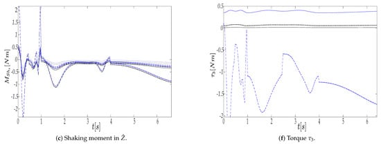
Figure 9.
Behavior of the shaking force , shaking moment , and torque for the designs with different velocities and two different end-effector masses in the linear trajectory. The design behaviors associated with kg are described in lines as  RBD, DBD, DTBD, SMBD,
 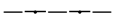 SFBD. The design behaviors associated with kg are described in lines as
  RBD, DBD, DTBD, SMBD,
  SFBD.
SFBD.
RBD, DBD, DTBD, SMBD, SFBD. The design behaviors associated with kg are described in lines as RBD, DBD, DTBD, SMBD, SFBD.

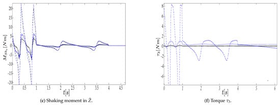
Figure 10.
Behavior of the shaking force , shaking moment , and torque for the designs with different velocities and two different end-effector masses in the circular trajectory. The design behaviors associated with kg are described in lines as RBD, DBD, DTBD, SMBD, SFBD. The design behaviors associated with kg are described in lines as RBD, DBD, DTBD, SMBD, SFBD.
RBD, DBD, DTBD, SMBD, SFBD. The design behaviors associated with kg are described in lines as RBD, DBD, DTBD, SMBD, SFBD.

Figure 11.
Behavior of the shaking force , shaking moment , and torque for the designs with different velocities and two different end-effector masses in the lemniscate trajectory. The design behaviors associated with kg are described in lines as RBD, DBD, DTBD, SMBD, SFBD. The design behaviors associated with kg are described in lines as RBD, DBD, DTBD, SMBD, SFBD.
RBD, DBD, DTBD, SMBD, SFBD. The design behaviors associated with kg are described in lines as RBD, DBD, DTBD, SMBD, SFBD.

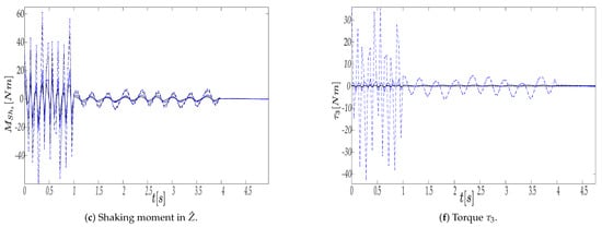
Figure 12.
Behavior of the shaking force , shaking moment , and torque for the designs with different velocities and two different end-effector masses in the hypocycloid trajectory. The design behaviors associated with kg are described in lines as RBD, DBD, DTBD, SMBD, SFBD. The design behaviors associated with kg are described in lines as RBD, DBD, DTBD, SMBD, SFBD.
RBD, DBD, DTBD, SMBD, SFBD. The design behaviors associated with kg are described in lines as RBD, DBD, DTBD, SMBD, SFBD.
The overall findings on the number of wins for each indicator shown in Table 8, Table 9, Table 10 and Table 11 are summarized in Table 12. The first term () of the results given in the form () indicates the percentage sum of the win number for the RMS value comparative results for every indicator (shaking force, shaking moment, and torque) on each execution time for the four trajectories. The second term () provides the percentage sum of the win number in the mean variations of such indicators. The numerical results of the summarized Table 12 show the following:
- The proposed RBD presents the slightest variations for the three indicators in the comparison with DBD, DTBD, and SMBD (see values for the RBD in the three columns of indicators), but not the comparison with SFBD, which is only robust in the shaking force balancing. Thus, the RBD obtained a high degree of robustness under the effect of mass variations.
- Regarding the torque indicator, the RBD significantly decreases the torque in comparison to the other designs (see values for the RBD in the third column ).
- As expected, the RBD outperforms the SMBD in the shaking force indicator with but performs poorly in the shaking moment indicator with because the latter is only concerned with fulfilling the shaking moment. Similar behavior emerges with the comparative results of the RBD with respect to the SFBD, where the former is better in the shaking moment indicator with , and the latter is better in the shaking force indicator with (which is the main objective to satisfy in the SFBD).
- It is also observed that the proposed RBD presents the worst performance in the shaking force and shaking moment with respect to the DBD and the DTBD (see the first and second columns), but, as commented previously, the RBD has superior performance in the torque and their three mean variations (in four out of the six indicators). This behavior is expected because the DBD and the DTBD simultaneously incorporate two or three of the design’s performance functions. Nevertheless, in spite of the DBD and the DTBD having a smaller value in those indicators without end-effector mass, these indicators present a similar value when the mass changes, indicating that the RBD presents suitable performance in such indicators under mass variations.
- Considering the three indicators and their three mean variations in Table 12 (related to the six objective functions to be optimized in the proposal), the RBD presents a superior percentage in four out of the six indicators when it is compared with the DBD and DTBD. In the case of the comparison with the SMBD, the RBD shows a percentage improvement in five out of the six indicators. When the RBD is compared with the SFBD, four metrics show a superior value or an equal percentage (in one of them, it ties). These results indicate that the proposed RBD shows improved behavior with shifting masses, and the proposed formulation can also handle different trajectories and speeds.
5. Conclusions
In this work, a robust design approach is proposed for balancing the shaking force, the shaking moment, and the torque of robotic manipulators. This approach is stated as a constrained multiobjective optimization problem, where the time-independent terms of the shaking force balancing, shaking moment balancing, and torque as well as their variations are proposed as objective functions. The link shape requirement, the motor position condition, and the limits of the design variable vector are the design constraints. The design approach is applied to a particular three-degree-of-freedom parallel-serial manipulator, where 1023 Pareto solutions are obtained through NSGA-II.
The comparative results of the performance function changes with different loads () in the end-effector of the robot indicate that the RBD presents an outstanding reduction in the time-independent terms of the shaking force balancing around , shaking moment balancing around , and torque around with respect to DBD. Thus, the performance function is less influenced by the load parameters because of the reductions in their sensitivities.
On the other hand, the comparative empirical evidence with the RMS values of the shaking force, shaking moment, and torque indicates the following with respect to other design approaches. The selected tradeoff in the obtained Pareto front (named RBD) considerably reduces the variations (sensitivities) in the shaking force, the shaking moment, and the torque with changes in the end-effector mass and through applications that require different speeds and shapes of the trajectory to be performed. In particular, under 60 numerical simulations per design, when the RBD is compared with the DBD, an average of of the results improve the sensitivities in the shaking force, the shaking moment, and the torque. When the RBD is compared with the DTBD, an average of of results decrease their sensitivities. When the RBD is compared with the SFBD, it obtains a tie () in the average of the decrement in the sensitivity. The comparison of the RBD with respect to the SMBD indicates that an average of of the results have improved the sensitivities in the shaking force, the shaking moment, and the torque.
It is also observed that the RBD reduces the applied torque in the interval with respect to the compared mechanisms.
The results also show that the obtained RBD exceeds the performance in the shaking force, the shaking moment, the torque, and its variations when it is compared with the approaches of SFBD or SMBD, i.e., the RBD reduces the torque in , the shaking moment in , and provides competitive average sensitivities in , or the torque in , the shaking force in , and the sensitivities in , when it is compared with approaches that focus on the fulfillment of one balancing condition (shaking force or shaking moment), respectively.
In the case of the comparative results with the DBD and DTBD, the proposed RBD presents superior performance in the torque delivery and in the robustness of the shaking force, shaking moment, and torque (in four out of the six indicators). Thus, the RBD presents a better tradeoff among metrics.
Finally, the proposed design approach can be extended to mechanisms and other robotic manipulators with more degrees of freedom.
One limitation of the proposal is that the tradeoff is tied to how well and efficiently the optimizer works. Thus, future work will include the addition of operators to multiobjective evolutionary algorithms that encourage exploration and exploitation to find different and notable tradeoffs that are better than the obtained metrics in the DBD and DTBD. Another future work option is to come up with a design strategy in which the size of loads or linkages is usually spread around a known mean value and variance. This is also a safe assumption in real-world situations. Future research may also examine the incorporation of vibration sources connected to the elastodynamics of the transmission, couplings, and mechanism components [59,60]. Experimental verification of the proposed RBD approach is also another area for future work.
Author Contributions
Conceptualization, formal analysis, investigation, visualization, R.M.-R., M.G.V.-C. and A.R.-M.; data curation, software, validation, R.M.-R., A.R.-M. and J.H.P.-C.; methodology, R.M.-R., V.M.S.-G. and M.G.V.-C.; writing—original draft preparation, writing—review and editing, R.M.-R. and M.G.V.-C.; Resources, V.M.S.-G. and M.G.V.-C.; supervision, project administration, funding acquisition, M.G.V.-C. All authors have read and agreed to the published version of the manuscript.
Funding
This research was funded by the Secretaría de Investigación y Posgrado (SIP) of the Instituto Politécnico Nacional under Grant 20220255 and 20230320.
Institutional Review Board Statement
Not applicable.
Informed Consent Statement
Not applicable.
Data Availability Statement
Data are available on request from the corresponding author.
Acknowledgments
The authors acknowledge the support of the Secretaría de Investigación y Posgrado (SIP) of the Instituto Politécnico Nacional, and CONACYT. The first author acknowledges the support of the Consejo Nacional de Ciencia y Tecnología (CONACyT) in Mexico through a scholarship to pursue graduate studies at CIDETEC-IPN.
Conflicts of Interest
The authors declare no conflict of interest.
Abbreviations
The following abbreviations are used in this manuscript:
| Acronyms | |
| TITShFB | The Time-Independent Terms of the Shaking Force Balancing |
| TITShMB | The Time-Independent Terms of the Shaking Moment Balancing |
| TITAT | The Time-Independent Terms of the Applied Torque |
| RBD | Robust Balancing Design |
| DBD | Dynamic Balancing Design |
| SFBD | Shaking Force Balancing Design |
| SMBD | Shaking Moment Balancing Design |
| DTBD | Dynamic and Torque Balancing Design |
| GA | Genetic Algorithm |
| SQP | Sequential Quadratic Programming |
| MOGA | Multiobjective Genetic Algorithm |
| G.C.M. | Global Center of Mass |
| NLC-MOP | Nonlinear Constrained Multiobjective Optimization Problem |
| DE | Differential Evolution |
| NSGA-II | Non-Dominated Sorting Genetic Algorithm II |
| RMS | Root Mean Square |
| SBX | Simulated Binary Crossover |
| NP | Number of Individuals in the Population |
| Nomenclature | |
| J | The weighted objective function for the |
| non-robust balancing approach | |
| The i-th objective function for the | |
| non-robust balancing approach | |
| The objective function vector for the | |
| robust balancing approach | |
| The i-th design objective variation with respect | |
| to the j-th uncertainty | |
| Design objective number | |
| Design variable vector | |
| The j-th constraint | |
| Inequality constraint number | |
| Angular position vector | |
| Angular velocity vector | |
| Angular acceleration vector | |
| Torque vector | |
| The i-th torque | |
| The i-th link | |
| Polar coordinates of the i-th link mass center | |
| with respect to coordinate system | |
| Cartesian coordinate of the i-th link | |
| mass center with respect to coordinate system | |
| The i-th inertia tensor | |
| The i-th mass | |
| The i-th fixed link length | |
| The mass center of the i-th link | |
| Total mass center vector | |
| Shaking force vector | |
| Shaking moment vector | |
| Total mass center time-independent terms | |
| grouped in a matrix | |
| Total mass center time-dependent terms | |
| grouped in a vector | |
| Angular momentum in the z axis | |
| Shaking moment time-independent terms | |
| grouped in a vector | |
| Angular momentum time-dependent terms | |
| grouped in a vector | |
| Inertia matrix time-dependent terms | |
| grouped in a matrix | |
| Inertia matrix time-independent terms | |
| grouped in a matrix | |
| Centrifugal and Coriolis forces time-dependent | |
| terms grouped in a matrix | |
| Centrifugal and Coriolis forces time-independent | |
| terms grouped in a matrix | |
| Gravity time-dependent terms | |
| grouped in a vector | |
| Gravity time-independent terms | |
| grouped in a matrix | |
| The i-th inertia tensor | |
| T | Period of a trajectory |
| The angular velocity vector of the i-th link | |
| Extra mass in the end-effector | |
| Inertia tensor of the extra mass | |
| n | Number of degrees of freedom |
| Inertia matrix of the robot | |
| Centrifugal and Coriolis forces matrix of | |
| the robot | |
| Gravity vector of the robot | |
| Variation in the i-th objective function | |
| Crossover probability | |
| Mutation probability | |
| Distribution index for crossover | |
| Distribution index for mutation | |
| Set of simple geometries of the i-th link | |
| Design objective weight | |
| Lower limit of the design parameter vector | |
| Upper limit of the design parameter vector | |
| Uncertain parameter vector | |
| Uncertain parameter nominal value vector | |
| Variation in from | |
| The i-th uncertain parameter nominal value | |
| The i-th uncertain parameter change | |
| , | Cartesian position and orientation |
| of the robot end-effector with respect to | |
| coordinate system | |
| g | Gravity acceleration |
| The i-th angular velocity | |
| The i-th angular position | |
| The i-th coordinate of the link system | |
| Mass of the third actuator | |
| Cartesian position of the third actuator | |
| Distance added to the fourth link | |
| Geometric variables of the shape | |
| for the i-th link | |
| Simple geometries of the shape for the i-th link | |
| Those that form the set | |
| A hole (cylinder) in the fourth link. For ∀ , | |
| the hole is not considered. | |
| Frobenius norm of the matrix • | |
| Maximum allowed link height | |
| Maximum allowed link width | |
| Tolerance of the link radius | |
| r | The hole radius in the cylinder (holes) , |
| and , | |
| The aluminum density | |
| The motor radius | |
| The motor mass | |
| The i-th diagonal line that constrains | |
| the motor placement | |
| Parent population at the generation G | |
| The i-th random variable between | |
| Sum of normalized constraint distance | |
| of the i-th chromosome | |
| , | Maximum or minimum number between a and b |
| G | Generation number |
| Maximum generation number | |
| Child vector a | |
| Child population |
Appendix A. Parameters of the Simple Geometry in Ωi
The mass , the mass center length expressed in Cartesian coordinates (with respect to the coordinate system ), and the inertia moment in the z axis of each simple geometry in are given as follows.
Appendix B. Detailed Description of the Matrices M, C and the Vector G
The elements , and ∀, associated with the closed-form dynamic model (22) are detailed below.
Appendix C. Detailed Description of the Sub-Matrices in the Matrices M, C and the Vector G
The elements of the matrices , and in (23) and (24) and the vectors and are detailed in this section.
References
- Aivaliotis, P.; Arkouli, Z.; Georgoulias, K.; Makris, S. Degradation curves integration in physics-based models: Towards the predictive maintenance of industrial robots. Robot.-Comput.-Integr. Manuf. 2021, 71, 102177. [Google Scholar] [CrossRef]
- Martini, A.; Troncossi, M.; Rivola, A. Algorithm for the static balancing of serial and parallel mechanisms combining counterweights and springs: Generation, assessment and ranking of effective design variants. Mech. Mach. Theory 2019, 137, 336–354. [Google Scholar] [CrossRef]
- Mottola, G.; Cocconcelli, M.; Rubini, R.; Carricato, M. Gravity Balancing of Parallel Robots by Constant-Force Generators. In Gravity Compensation in Robotics; Arakelian, V., Ed.; Springer International Publishing: Cham, Switzerland, 2022; pp. 229–273. [Google Scholar] [CrossRef]
- Bagci, C. Shaking force balancing of planar linkages with force transmission irregularities using balancing idler loops. Mech. Mach. Theory 1979, 14, 267–284. [Google Scholar] [CrossRef]
- Arakelian, V.; Dahan, M.; Smith, M. A Historical Review of the Evolution of the Theory on Balancing of Mechanisms. In Proceedings of the International Symposium on History of Machines and Mechanisms Proceedings HMM, Cassino, Italy, 11–13 May 2000; Ceccarelli, M., Ed.; Springer: Dordrecht, The Netherlands, 2000; pp. 291–300. [Google Scholar]
- Lowen, G.; Berkof, R. Survey of investigations into the balancing of linkages. J. Mech. 1968, 3, 221–231. [Google Scholar] [CrossRef]
- Berkof, R.S.; Lowen, G.G. A New Method for Completely Force Balancing Simple Linkages. J. Eng. Ind. 1969, 91, 21–26. [Google Scholar] [CrossRef]
- Berkof, R.S.; Lowen, G.G. Theory of Shaking Moment Optimization of Force-Balanced Four-Bar Linkages. J. Eng. Ind. 1971, 93, 53–60. [Google Scholar] [CrossRef]
- Berkof, R.S. Complete force and moment balancing of inline four-bar linkages. Mech. Mach. Theory 1973, 8, 397–410. [Google Scholar] [CrossRef]
- On the Development of Reactionless Parallel Manipulators, Vol. Volume 7A: 26th Biennial Mechanisms and Robotics Conference, International Design Engineering Technical Conferences and Computers and Information in Engineering Conference. 2000. Available online: https://asmedigitalcollection.asme.org/IDETC-CIE/proceedings-pdf/IDETC-CIE2000/35173/493/6610082/493_1.pdf (accessed on 23 December 2020). [CrossRef]
- Orvañanos-Guerrero, M.; Sánchez, C.; Rivera, M.; Acevedo, M.; Velázquez, R. Gradient Descent-Based Optimization Method of a Four-Bar Mechanism Using Fully Cartesian Coordinates. Appl. Sci. 2019, 9, 4115. [Google Scholar] [CrossRef]
- Arakelian, V.; Briot, S. Balancing of Linkages and Robot Manipulators: Advanced Methods with Illustrative Examples; Springer: Cham, Switzerland, 2015. [Google Scholar] [CrossRef]
- van der Wijk, V.; Herder, J.L.; Demeulenaere, B. Comparison of Various Dynamic Balancing Principles Regarding Additional Mass and Additional Inertia. J. Mech. Robot. 2009, 1, 041006. [Google Scholar] [CrossRef]
- Kochev, I. General theory of complete shaking moment balancing of planar linkages: A critical review. Mech. Mach. Theory 2000, 35, 1501–1514. [Google Scholar] [CrossRef]
- Lowen, G.; Tepper, F.; Berkof, R. The quantitative influence of complete force balancing on the forces and moments of certain families of four-bar linkages. Mech. Mach. Theory 1974, 9, 299–323. [Google Scholar] [CrossRef]
- Feng, G. Complete shaking force and shaking moment balancing of 17 types of eight-bar linkages only with revolute pairs. Mech. Mach. Theory 1991, 26, 197–206. [Google Scholar] [CrossRef]
- Xi, F. Dynamic balancing of hexapods for high-speed applications. Robotica 1999, 17, 335–342. [Google Scholar] [CrossRef]
- Herder, J.; Gosselin, C. A counter-rotary counterweight (CRCW) for light-weight dynamic balancing. In Proceedings of the DETC2004: Proceedings of the ASME 2004 Design Engineering Technical Conferences and Computers and Information in Engineering Conference, Salt Lake City, UT, USA, 28 September–2 October 2004; ASME: New York, NY, USA, 2004; pp. 1–9. [Google Scholar]
- Arakelian, V.H.; Smith, M.R. Shaking Force and Shaking Moment Balancing of Mechanisms: A Historical Review with New Examples. J. Mech. Des. 2005, 127, 334–339. [Google Scholar] [CrossRef]
- van der Wijk, V.; Herder, J.L. Synthesis of Dynamically Balanced Mechanisms by Using Counter-Rotary Countermass Balanced Double Pendula. J. Mech. Des. 2009, 131, 111003. [Google Scholar] [CrossRef]
- Farmani, M.R.; Jaamialahmadi, A.; Babaie, M. Multiobjective optimization for force and moment balance of a four-bar linkage using evolutionary algorithms. J. Mech. Sci. Technol. 2011, 25, 2971–2977. [Google Scholar] [CrossRef]
- Zhang, D.; Wei, B. Dynamic Balancing of Mechanisms and Synthesizing of Parallel Robots; Springer: Cham, Switzerland, 2016. [Google Scholar]
- Jong, J.D.; Dijk, J.V.; Herder, J. A screw based methodology for instantaneous dynamic balance. Mech. Mach. Theory 2019, 141, 267–282. [Google Scholar] [CrossRef]
- Chaudhary, H.; Saha, S.K. An optimization technique for the balancing of spatial mechanisms. Mech. Mach. Theory 2008, 43, 506–522. [Google Scholar] [CrossRef]
- Gupta, V.; Saha, S.K.; Chaudhary, H. Optimum Design of Serial Robots. J. Mech. Des. 2019, 141, 082303. [Google Scholar] [CrossRef]
- Agrawal, S.K.; Fattah, A. Reactionless space and ground robots: Novel designs and concept studies. Mech. Mach. Theory 2004, 39, 25–40. [Google Scholar] [CrossRef]
- van der Wijk, V.; Demeulenaere, B.; Gosselin, C.; Herder, J.L. Comparative Analysis for Low-Mass and Low-Inertia Dynamic Balancing of Mechanisms. J. Mech. Robot. 2012, 4, 031008. [Google Scholar] [CrossRef]
- Fattah, A.; Agrawal, S.K. On the design of reactionless 3-DOF planar parallel mechanisms. Mech. Mach. Theory 2006, 41, 70–82. [Google Scholar] [CrossRef]
- Papadopoulos, E.; Abu-Abed, A. Design and motion planning for a zero-reaction manipulator. In Proceedings of the 1994 IEEE International Conference on Robotics and Automation, San Diego, CA, USA, 8–13 May 1994; Volume 2, pp. 1554–1559. [Google Scholar] [CrossRef]
- van der Wijk, V. Methodology for Analysis and Synthesis of Inherently Force and Moment-Balanced Mechanisms. Ph.D. Thesis, University of Twente, Enschede, The Netherlands, 2014. [Google Scholar] [CrossRef]
- Fattah, A.; Agrawal, S.K. Design and simulation of a class of spatial reactionless manipulators. Robotica 2005, 23, 75–81. [Google Scholar] [CrossRef]
- Gosselin, C.; Vollmer, F.; Cote, G.; Wu, Y. Synthesis and design of reactionless three-degree-of-freedom parallel mechanisms. IEEE Trans. Robot. Autom. 2004, 20, 191–199. [Google Scholar] [CrossRef]
- Wu, Y.; Gosselin, C.M. Synthesis of Reactionless Spatial 3-DoF and 6-DoF Mechanisms without Separate Counter-Rotations. Int. J. Robot. Res. 2004, 23, 625–642. [Google Scholar] [CrossRef]
- Briot, S.; Arakelian, V. Complete shaking force and shaking moment balancing of in-line four-bar linkages by adding a class-two RRR or RRP Assur group. Mech. Mach. Theory 2012, 57, 13–26. [Google Scholar] [CrossRef]
- de Jong, J.; Müller, A.; Herder, J. Higher-order derivatives of rigid body dynamics with application to the dynamic balance of spatial linkages. Mech. Mach. Theory 2021, 155, 104059. [Google Scholar] [CrossRef]
- Ye, Z.; Smith, M. Complete balancing of planar linkages by an equivalence method. Mech. Mach. Theory 1994, 29, 701–712. [Google Scholar] [CrossRef]
- Alici, G.; Shirinzadeh, B. Optimum force balancing of a planar parallel manipulator. Proc. Inst. Mech. Eng. Part C J. Mech. Eng. Sci. 2003, 217, 515–524. [Google Scholar] [CrossRef]
- Laliberté, T.; Gosselin, C. Synthesis, optimization and experimental validation of reactionless two-DOF parallel mechanisms using counter-mechanisms. Meccanica 2016, 51, 3211–3225. [Google Scholar] [CrossRef]
- Ur-Rehman, R.; Caro, S.; Chablat, D.; Wenger, P. Multi-objective path placement optimization of parallel kinematics machines based on energy consumption, shaking forces and maximum actuator torques: Application to the Orthoglide. Mech. Mach. Theory 2010, 45, 1125–1141. [Google Scholar] [CrossRef]
- Chaudhary, K.; Chaudhary, H. Optimal dynamic balancing and shape synthesis of links in planar mechanisms. Mech. Mach. Theory 2015, 93, 127–146. [Google Scholar] [CrossRef]
- Chaudhary, H.; Saha, S. Equimomental System and Its Applications; ASME: New York, NY, USA, 2006; Volume 2006. [Google Scholar] [CrossRef]
- Chaudhary, H.; Saha, S. Dynamics and Balancing of Multibody Systems; Springer: Berlin, Germany, 2009. [Google Scholar] [CrossRef]
- Alici, G.; Shirinzadeh, B. Optimum dynamic balancing of planar parallel manipulators based on sensitivity analysis. Mech. Mach. Theory 2006, 41, 1520–1532. [Google Scholar] [CrossRef]
- Yu, H.; Qian, Z.; Borugadda, A.; Sun, W.; Zhang, W. Partial Shaking Moment Balancing of Spherical Parallel Robots by a Combined Counterweight and Adjusting Kinematic Parameters Approach. Machines 2022, 10, 216. [Google Scholar] [CrossRef]
- Ouyang, P.; Li, Q.; Zhang, W. Integrated design of robotic mechanisms for force balancing and trajectory tracking. Mechatronics 2003, 13, 887–905. [Google Scholar] [CrossRef]
- Ouyang, P.R.; Zhang, W.J. Force Balancing of Robotic Mechanisms Based on Adjustment of Kinematic Parameters. J. Mech. Des. 2004, 127, 433–440. [Google Scholar] [CrossRef]
- Mejia-Rodriguez, R.; Villarreal-Cervantes, M.G.; Martínez-Castelán, J.N.; Muñoz-Reina, J.S.; Silva-García, V.M. Optimal dynamic balancing of a hybrid serial-parallel robotic manipulator through bio-inspired computing. J. King Saud Univ.-Eng. Sci. 2021; In Press. [Google Scholar] [CrossRef]
- Ilia, D.; Sinatra, R. A novel formulation of the dynamic balancing of five-bar linkages with applications to link optimization. Multibody Syst. Dyn. 2009, 21, 193–211. [Google Scholar] [CrossRef]
- Demeulenaere, B.; Verschuure, M.; Swevers, J.; Schutter, J.D. A General and Numerically Efficient Framework to Design Sector-Type and Cylindrical Counterweights for Balancing of Planar Linkages. J. Mech. Des. 2010, 132, 011002. [Google Scholar] [CrossRef]
- Erkaya, S. Investigation of balancing problem for a planar mechanism using genetic algorithm. J. Mech. Sci. Technol. 2013, 27, 2153–2160. [Google Scholar] [CrossRef]
- Chaudhary, K.; Chaudhary, H. Dynamic balancing of planar mechanisms using genetic algorithm. J. Mech. Sci. Technol. 2014, 28, 4213–4220. [Google Scholar] [CrossRef]
- Kim, J. Task based kinematic design of a two DOF manipulator with a parallelogram five-bar link mechanism. Mechatronics 2006, 16, 323–329. [Google Scholar] [CrossRef]
- Saravanan, R.; Ramabalan, S.; Babu, P.D. Optimum static balancing of an industrial robot mechanism. Eng. Appl. Artif. Intell. 2008, 21, 824–834. [Google Scholar] [CrossRef]
- Deb, K.; Pratap, A.; Agarwal, S.; Meyarivan, T. A fast and elitist multiobjective genetic algorithm: NSGA-II. IEEE Trans. Evol. Comput. 2002, 6, 182–197. [Google Scholar] [CrossRef]
- Osyczka, A. Multicriterion Optimization in Engineering with FORTRAN Programs; Ellis Horwood-Wiley: Chichester, UK, 1984. [Google Scholar]
- Juárez-Castillo, E.; Acosta-Mesa, H.G.; Mezura-Montes, E. Empirical study of bound constraint-handling methods in Particle Swarm Optimization for constrained search spaces. In Proceedings of the 2017 IEEE Congress on Evolutionary Computation (CEC), Donostia, Spain, 5–8 June 2017; pp. 604–611. [Google Scholar] [CrossRef]
- Gosselin, C. Gravity Compensation, Static Balancing and Dynamic Balancing of Parallel Mechanisms. In Smart Devices and Machines for Advanced Manufacturing; John Wiley & Sons, Inc.: New York, NY, USA, 2008. [Google Scholar] [CrossRef]
- Spong, M.W.; Hutchinson, S.; Vidyasagar, M. Robot Modeling and Control; John Wiley & Sons, Inc.: New York, NY, USA, 2005. [Google Scholar] [CrossRef]
- Martini, A.; Troncossi, M.; Rivola, A. Elastodynamic Effects of Mass-Balancing: Experimental Investigation of a Four-Bar Linkage. Adv. Mech. Eng. 2013, 5, 949457. [Google Scholar] [CrossRef]
- Raghu, E.; Balasubramonian, A. Experimental Study on the Elastodynamic Behavior of the Unbalanced and the Counterweighted Four Bar Mechanisms. J. Mech. Des. 1990, 112, 271–277. [Google Scholar] [CrossRef]
Disclaimer/Publisher’s Note: The statements, opinions and data contained in all publications are solely those of the individual author(s) and contributor(s) and not of MDPI and/or the editor(s). MDPI and/or the editor(s) disclaim responsibility for any injury to people or property resulting from any ideas, methods, instructions or products referred to in the content. |
© 2023 by the authors. Licensee MDPI, Basel, Switzerland. This article is an open access article distributed under the terms and conditions of the Creative Commons Attribution (CC BY) license (https://creativecommons.org/licenses/by/4.0/).