Article

Fourier Graph Convolution Network for Time Series Prediction

1
Fujian Provincial Universities Engineering Research Center for Intelligent Driving Technology, School of Transportation, Fujian University of Technology, Fuzhou 350118, China
2
Department of Computing Science, University of Aberdeen, Aberdeen AB24 3UE, UK
*
Author to whom correspondence should be addressed.
Mathematics 2023, 11(7), 1649; https://doi.org/10.3390/math11071649
Submission received: 28 February 2023 / Revised: 20 March 2023 / Accepted: 23 March 2023 / Published: 29 March 2023

Abstract

:
The spatio-temporal pattern recognition of time series data is critical to developing intelligent transportation systems. Traffic flow data are time series that exhibit patterns of periodicity and volatility. A novel robust Fourier Graph Convolution Network model is proposed to learn these patterns effectively. The model includes a Fourier Embedding module and a stackable Spatial-Temporal ChebyNet layer. The development of the Fourier Embedding module is based on the analysis of Fourier series theory and can capture periodicity features. The Spatial-Temporal ChebyNet layer is designed to model traffic flow’s volatility features for improving the system’s robustness. The Fourier Embedding module represents a periodic function with a Fourier series that can find the optimal coefficient and optimal frequency parameters. The Spatial-Temporal ChebyNet layer consists of a Fine-grained Volatility Module and a Temporal Volatility Module. Experiments in terms of prediction accuracy using two open datasets show the proposed model outperforms the state-of-the-art methods significantly.

1. Introduction

Intelligent Transportation Systems (ITS) aim to establish a complete traffic management system and provide innovative services for traffic management departments through the research of basic traffic theory and the integration of advanced science and technology [1,2]. In Intelligent Transportation Systems (ITS), one of the critical issues is traffic flow prediction. Accurate traffic flow prediction is vital in many scenarios, such as road resource management, traffic network optimization, and traffic congestion alleviation [3,4]. However, actual traffic flow presents a complex mixture of periodicity and uncertainty. For example, traffic flow data are collected from sensors on the road, so the data shows periodic changes due to the regular activities of individuals, such as daily traffic peak periods. Meanwhile, abundant factors contribute to uncertainty in traffic flow data [5], such as weather conditions, unexpected accidents, and road maintenance. In addition, traffic flow data cannot be fully collected due to the burdensome cost, which further increases the complexity of the traffic flow prediction problem. Therefore, there remains a series of crucial challenges to extract patterns from complicated traffic flow and then make reliable predictions based on them.
Many emerging methods are dedicated to traffic flow prediction. As classical statistical methods, Autoregressive Integrated Moving Average (ARIMA) models are applied in stationary time series where the traffic flow prediction could also be regarded as a seasonal ARIMA process [6]. Further, Autoregressive Conditional Heteroskedasticity (ARCH) [7] has been proposed to analyze heteroskedasticity in time series. Nevertheless, these classical methods have significant drawbacks in dynamically processing various complex requirements for traffic flow prediction. Advanced artificial intelligence technology [8,9] improves the prediction accuracy of traffic flow. The Graph Convolution Network (GCN) has recently drawn attention due to its powerful ability to capture spatiotemporal information. Its typical variations include Temporal Graph Convolutional Network (T-GCN) [10], Attention-based Spatial-Temporal Graph Convolution Network (ASTGCN) [11], Spatial-Temporal Synchronous Graph Convolutional Networks (STSGCN) [12], and Dynamic Graph Convolution Network (DGCN) [3]. These models regard the actual traffic flow as an entity for prediction. As the preliminary work, an improved Dynamic Chebyshev Graph Convolution Network (iGCGCN) has been proposed [13] to enhance the attention mechanism and the data construction.
Based on the decomposition of time series data, traffic flow data can consist of several components. For example, modules, including the Time-Series Analysis and Supervised-Learning (TSA-SL) [14] and the hybrid model [15], try to decompose the traffic flow into two main parts, periodicity and volatility, and further learn the two parts separately to improve the prediction accuracy. Figure 1a illustrates the original traffic flow of three detectors, and each detector has a specific periodicity fluctuation associated with the dynamic traffic network. Figure 1b–d show the corresponding decomposition results of detector1 data, including trend, periodicity, and volatility. Trends may be stable, uptrend, or downtrend, and the red circle in Figure 1b indicates a downtrend. In Figure 1c, the red box shows the change in one period of traffic flow data. In Figure 1d, the complicated dynamic volatility of detector1 is influenced by many factors, such as traffic patterns, the noise of traffic data, incomplete traffic flow, etc. Therefore, traffic flow forecasting models need the ability to automatically feature the components of various periodicities, trends, and volatility from the traffic flow data.
Although much effort has been devoted to the issue of traffic flow prediction, there are still some crucial challenges remaining in capturing the various periodicities and dynamic volatility.
  • The existing methods learn the periodicity based on frequency-domain methods, such as spectral analysis and traditional Fourier Transform [14,15,16,17]. These models generally require manual parameters and comply with rigorous assumptions, making these methods incapable of capturing various periodicities.
  • There is still a lack of an efficient way to learn dynamic volatility for improving robusticity, which is crucial to the dynamic spatial-temporal pattern recognition of the traffic network.
  • Some models capture periodicity and volatility, but these methods capture them independently and ignore their inherent relationship.
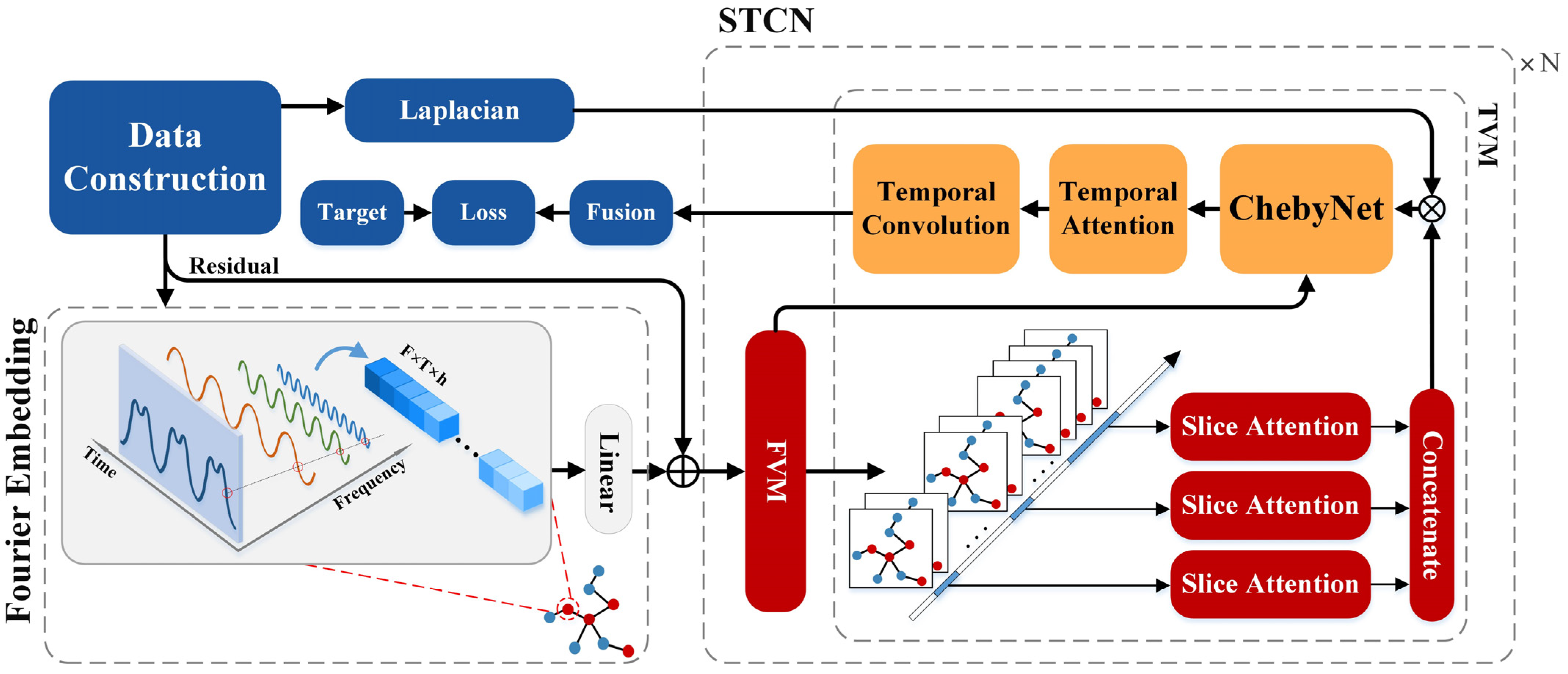
To address these issues, a robust Fourier Graph Convolution Network (F-GCN) architecture is proposed, which consists of two adaptive modules, including a Fourier Embedding (FE) and a stackable Spatial-Temporal ChebyNet (STCN) layer. The FE module is proposed to capture various periodicities without artificial intervention, and the STCN module with periodic embedding is developed to extract dynamic temporal volatility. The STCN is comprised of two sub-modules: a Fine-grained Volatility Module and a Temporal Volatility Module. In detail, the Fine-grained Volatility Module first captures the fine-grained volatility to decrease the difficulty of complex volatility learning. Then, the Temporal Volatility Module further captures the dynamic temporal volatility. Unlike independent learning periodicity and volatility, the F-GCN model can consider the correlation between the two parts.
The main contributions of this work are summarized as follows.
  • A novel Fourier Embedding module is proposed to capture periodicity patterns, which is proven to learn diversified periodicity patterns.
  • A stackable Spatial-Temporal ChebyNet layer, including a Fine-grained Volatility Module and a Temporal Volatility Module, is proposed to handle the complex volatility and learn dynamic temporal volatility for improving the system’s robusticity.
  • A dynamic Fourier Graph Convolution Network framework is proposed to integrate the periodicity and volatility analysis, which could be easily trained in an end-to-end method. Extensive experiments are conducted on several real-world traffic flow data, and the results significantly outperform state-of-the-art methods.
The remainder of this paper is constructed as follows. In Section 2, related studies are summarized in terms of traffic flow data decomposition and graph convolution network. Methods including preliminaries and the proposed model are given in detail in Section 3. Results and the Discussion are provided in Section 4. Finally, a summary is given in Section 5.

2. Literature Review

This section includes two subsections: traffic flow data decomposition and graph convolution network.

2.1. Traffic Flow Data Decomposition

Data decomposition has inspired many methods for improving the precision of traffic flow prediction. The procedure of these methods generally includes two independent phases. The traffic flow data are firstly decomposed into several parts, and then various algorithms are employed to learn traffic patterns from these decomposed parts. For example, a hybrid approach [15] for short-term traffic flow forecasting decomposes traffic flow data into periodic trends, deterministic parts, and volatility, then this method utilizes three different modules to learn patterns from their three components: the spectrum method, ARIMA, and an autoregressive model.
Remarkably, TSA-SL [14] regards traffic flow patterns as a combination of periodicity and volatility. Then, the traditional Fourier transform learns periodicity with manual parameters setting, and the conventional machine learning methods are employed to capture volatility. Further, a combination model [17] has been proposed to utilize Empirical Mode Decomposition (EMD) to disassemble the traffic flow into multiple components with different frequencies. After that, the ARIMA and the improved Extreme Learning Machine (ELM) are applied to learn these components. The method [16] utilizes an Ensemble Empirical Mode Decomposition (EEMD) and the artificial neural network layer for multi-scales traffic flow forecasting. These methods learn the decomposed parts using empirical methods, and the relationship among these parts is difficult to consider fully.

2.2. Graph Convolution Network

Traffic flow prediction is among the essential tasks in ITS, and many methods are applied to spatial-temporal prediction. Historical Average (HA) and ARIMA [6] are the conventional statistical approach to time series analysis for predicting traffic flow, and can only learn the linear relationship of the traffic network. With the advancement of machine learning, conventional machine learning algorithms have been developed to represent more complex and nonlinear data relationships. For example, some works introduced the Support Vector Regression (SVR) [18] and the Bayesian model [19] to capture high-dimensional nonlinear characteristics. Especially in recent years, deep learning has proven to be effective in various areas. Many deep learning models have been developed to predict traffic flow and improve performance. Convolution Neural Networks (CNN) and Gated Recurrent Unit networks (GRU) are commonly used to deal with spatial and temporal characteristics. For example, [20] employed 1D-CNN to learn the spatial features of traffic flow; [21] used bidirectional GRU for short-term traffic flow prediction, and ST-3DNet [22] constructed a 3D-CNN to capture traffic characteristics simultaneously in temporal and spatial dimensions. However, CNN-based methods require traffic flow to be structured data, which generally ignore the topology information of the road network.
With the extraordinary performance of deep learning in image and natural language processing, many researchers are devoted to dealing with graph structure with these methods. The Graph Neural Network has been proposed to model a graph structure, which could be summarized as follows. (1) Spectral Methods: Bruna et al. [23] initially introduced a graph convolutional network by generalizing the convolution kernel with the Laplacian matrix. Defferrard et al. [24] adopted Chebyshev polynomials to approximate eigenvalue decomposition with fewer parameters and significantly decrease computation complexity. Kipf et al. [25] proposed a first-order linear approximation of the graph convolutional model and further improved its computational efficiency. (2) Spatial ethods: Steven et al. [26] proposed an algorithm for undirected spatial graphs to update graphs with different distances. Unfortunately, the model parameters increase sharply for large-scale graphs. Niepert et al. [27] proposed converting graph structure data into traditional Euclidean data to overcome this drawback. William L et al. [28] proposed a general inductive reasoning framework to generate node representation through sampling and adjacent node characteristics.
With much effort from industry and academia, the graph neural network has gradually appeared in many variants to learn potential spatial-temporal patterns. MRes-RGNN [29] used residual recurrent graph neural networks to capture spatial-temporal information. ASTGCN [11] explores temporal and spatial relationships using an attention mechanism and a graph neural network. STSGCN [12] is used to build a module to capture local spatial and temporal characteristics and then stack this module along the time to learn long-term characteristics. Further, AGCRN [30] can automatically learn node features without pre-defined graphs using two adaptive modules. These methods have significantly improved the capacity to consider the relationship between nodes with the graph structure. Nevertheless, there is still a lack of an efficient way to automatically learn periodicity and volatility from traffic flow data.

3. Methods

3.1. Preliminaries

This section reviews the mathematical concepts used throughout the paper and serves as a reference for studying subsequent chapters.

3.1.1. The Complex Fourier Series

Signal Processing (SP) and communication engineering often apply Fourier theory. The Complex Fourier Series (CFS) representation of a periodic signal x t with period T can be written as Equation (1).
x t = k = X c k F s e j 2 π k F s t
where F s denotes the fundamental frequency and it equals 1 / T . The coefficients X c k F s are given by Equation (2).
X c k F s = 1 T T / 2 T / 2 x t e j 2 π k F s t d t
where X c k F s will be written as X c k , and is referred to as the complex Fourier series coefficient of x t .
The original Dirichlet Condition (DC) requires the signal to be Boundedly Varied (BV) over a period for CFS to converge. The CFS exists if x t satisfies the Dirichlet conditions that includes the condition in Equation (3).
T   x t d t <
or to the weaker condition in Equation (4).
T   x t 2 d t <
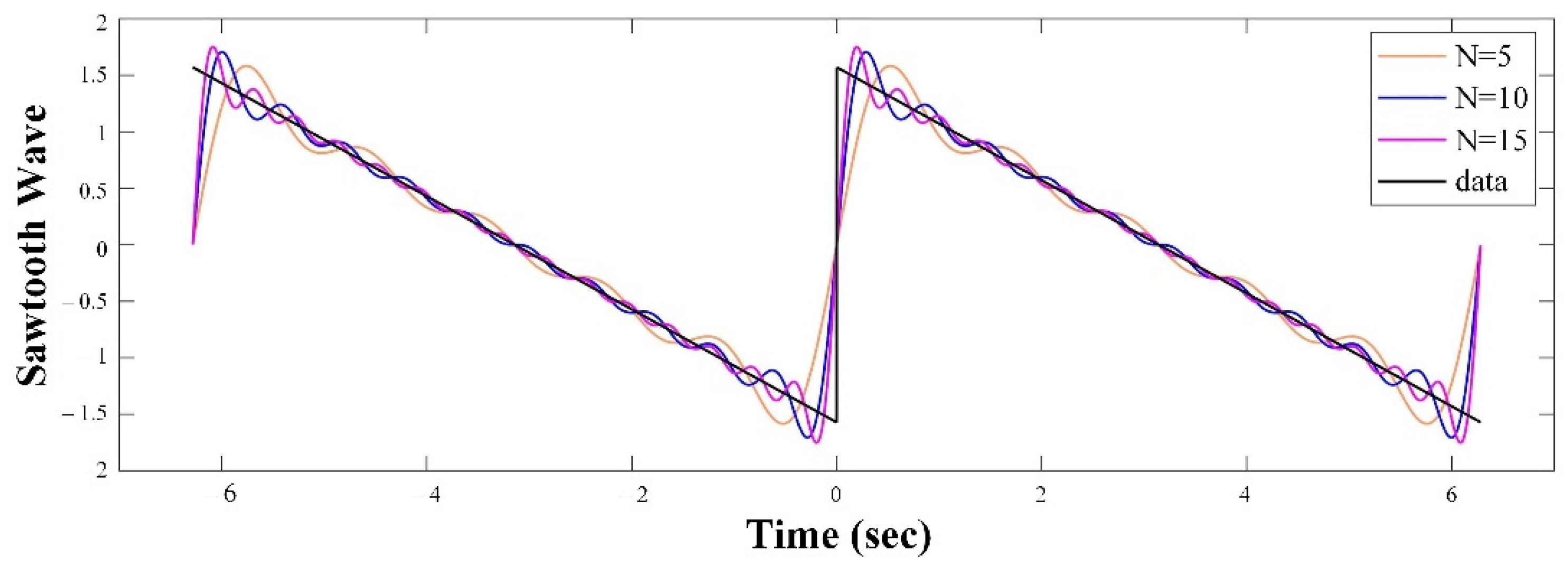
This condition is expressed as a signal with finite energy in one cycle. The sudden truncation of the Fourier series results in oscillations near the discontinuity. As the number of terms increases, the oscillation frequency increases while the amplitude decreases. However, the magnitude of the first ripple on either side of the discontinuity remains almost constant. This phenomenon was first discovered by A. Michelson and later explained mathematically by Gibbs. It occurs in all signal representations by a truncated number of orthogonal basis functions. An example is shown in Figure 2 in terms of the truncated Fourier series for the sawtooth wave function.

3.1.2. Real Fourier Series

Real Fourier series (RFS) coefficients are the real part of X c k , and can be written as in Equations (5)–(7).
X K = 2 T w k T / 2 T / 2 x t cos 2 π k F s t + θ k d t
w k = 1 / 2 , 1 , k = 0 o t h e r w i s e
θ k = 0 , π / 2 ,       k > 0       k < 0
where X ± k is sometimes referred to as the k t h harmonic. The inverse real Fourier series is given by Equation (8).
x t = k = X k cos 2 π k F s t + θ k
Equations (5) and (8) can also be written for k 0 as Equations (9)–(11).
X 1 k = w k 2 T T / 2 T / 2 x t cos 2 π k F s t d t
X 0 k = 2 T T / 2 T / 2 x t sin 2 π k F s t d t
and
x t = k = X 1 k cos 2 π k F s t + X 0 k sin 2 π k F s t
Thus, X k equals X 1 k for k 0 , and X 0 k for k < 0 . The Fourier series for the triangular wave has only the coefficients X 1 k . As shown in Figure 1b, the traffic flow is similar to the triangular wave.
Traffic Graph G : The traffic network is defined as an undirect graph G = V ,   E ,   A , where V is a set of nodes, V = N , and N is the number of nodes, E is a set of edges e i , j and e i , j represent the edge between node i and node j , A N × N denotes an original adjacent matrix of the network, and its calculation is given in Equation (12).
A i , j = { 1 , i f   e i , j 0 0 , i f   e i , j = 0
Time2Vec [31,32]: This model proposes a way of time embedding, and the learned embedding can be used for different architectures, as in Equation (13).
t 2 v τ i = ω i τ + φ i , i f   i = 0 cos ω i τ + φ i ,   i f   1 i k
where t 2 v τ i is the i t h element of t 2 v τ , τ represents the time scalar for different periodicity, ω i and φ i are the frequency and the phase-shift of the sine function, respectively, and are learnable parameters.
Spatial-Temporal Signal: The spatial graph signal is denoted as X G F × N , where F is the number of characteristics for the traffic graph, X G is extended along the time dimension, and the spatial-temporal graph signal is X G F × N × T , where T is the total number of time slices. The modeling in this work aims to discover the spatial and temporal patterns from massive traffic flow data.

3.1.3. Problem Statement

The traffic flow prediction problem can be described as follows. A mapping function is learned to map the historical spatial-temporal signal X G T h = X G t T h + 1 ,   , X G t 1 ,   X G t to a future spatial-temporal signal X G T f = X G t ,   X G t + 1 ,   , X G t + T f 1 , where T h is the length of historical data and T f is the length of target data.

3.2. Fourier Graph Convolution Network

The robust Fourier Graph Convolution Network (F-GCN) is described in this section. As shown in Figure 3, the architecture of F-GCN includes three primary modules: a data construction module, a Fourier Embedding (FE) module, and a stackable Spatial-Temporal ChebyNet (STCN) layer. First, the data construction module is employed to construct the graph containing three periodic data types and Laplacian. Then, the FE module learns various periodicity embedding for the graph. The stackable STCN is further utilized to explore the dynamic temporal volatility, and the loss values between the prediction and ground truth are calculated for backpropagation learning.

3.2.1. Data Construction

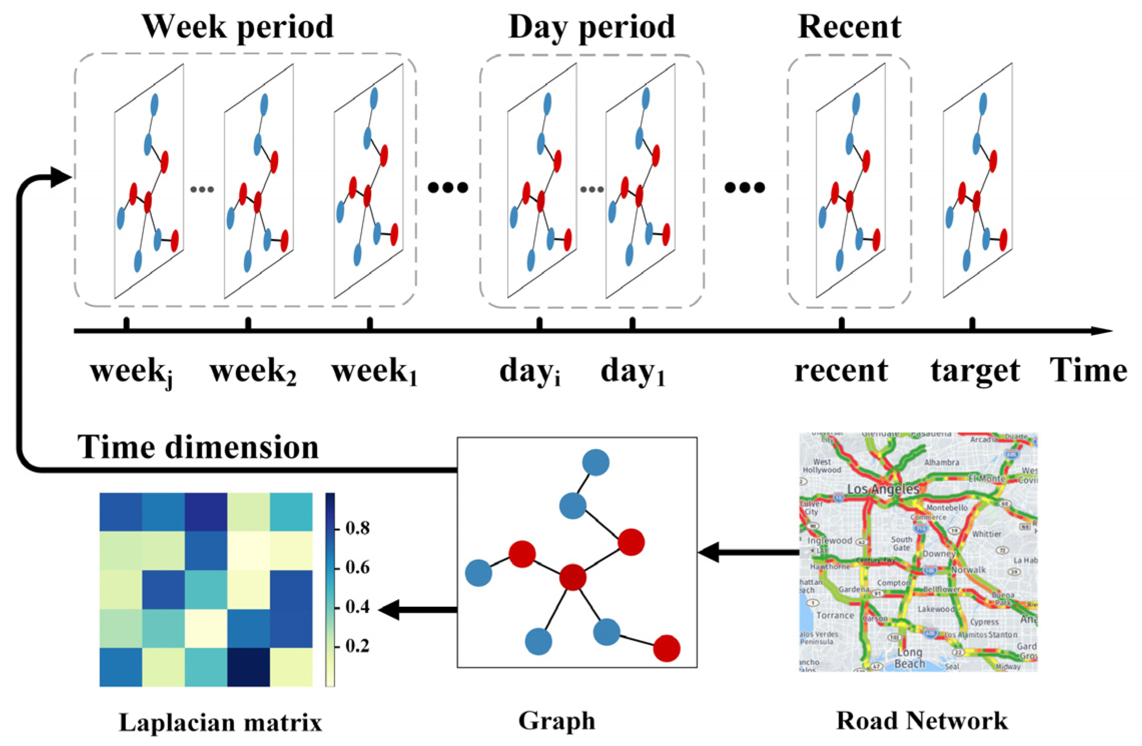
A flowchart of the data construction module is shown in Figure 4. As the system’s input, the traffic flow data are utilized to generate the Laplacian matrix and output a feature vector. Specifically, the actual traffic flow data produce a graph G , in which nodes represent sensors on the road network and edges are connections among sensors. According to the G , Laplacian matrix L = D A N × N is calculated, where D = j = 0 N A i , j N × N represents the degree matrix, and A is the adjacent matrix. In this work, three periods of traffic network are considered, including week-period X G T w = X G T w n , ,   X G T w 2 ,   X G T w 1 F × N × T w , day-period X G T d = X G T d n , ,   X G T d 2 ,   X G T d 1 F × N × T d , and recent-period X G T r = X G T r n , ,   X G T r 2 ,   X G T r 1 F × N × T r . Finally, the three periods are concatenated into X G = X G T w ,   X G T d ,   X G T r F × N × T , where [ ] denotes a concatenation operator, and T w + | T d + | T r = T .

3.2.2. Fourier Embedding

The traffic flow pattern generally presents various periodicities, making it highly complex to predict the traffic flow. To address this issue, traffic flow patterns are decomposed into two key elements: periodicity and volatility. A vector-based time representation method such as Time2Vec [31,32] is employed in other frameworks. Further, an operator E m b . , named Fourier Embedding (FE), is developed to capture various periodicities, which is shown in Equation (14). Known from the Fourier series theory [33], any periodic function can be obtained in this operator by superimposing multiple sine and cosine functions with different frequencies. Unlike traditionally decomposing methods, the proposed FE module is based on the embedding method, and could effectively represent various periodicities of traffic flow. The calculation is in Equation (14).
X G = E m b X G = X G W e F × N × T × d
where the E m b . operator is used to represent nodes of the graph, W e T × d is a learnable parameter, and d is the length of the vector embedding. X G comprises three periods of traffic flow, which help increase the adaptability for different periodicities. Meanwhile, it also provides more complex volatility possibilities, enabling downstream modules to explore volatility better.
As shown in Equation (11), the Fourier truncated series polynomials of order M can be presented in Equations (15) and(16).
F X G a 0 + m = 1 M a n c o s X G W m 1 + b n s i n X G W m 2
X G = F X G W f
where a 0 , a n T × T , b n T × T , W m 1 d × h , and W m 2 d × h are learnable parameters, c o s . and s i n . are trigonometric functions, F X G F × N × T × h is the result of periodicity embedding, W f h × 1 is a learnable parameter, and X G F × N × T is the output of the FE module.
The residual structure [34] is employed to learn the dynamic temporal volatility. The advantage of this structure is that the volatility in the original graph can be introduced into the downstream learning module in Equation (17).
X G res = X G + X G
where X G r e s F × N × T .

3.2.3. Spatial-Temporal ChebyNet Layer

A stackable Spatial-Temporal ChebyNet (STCN) layer is proposed to capture the dynamic temporal volatility. This layer includes two main components: a Fine-grained Volatility Module and Temporal Volatility Module.
A.
Fine-grained Volatility Module
As shown in Figure 1d, the volatility of the traffic flow is generally irregular and complicated. A Fine-grained Volatility Module is proposed in this work to represent the fine-grained volatility features for capturing complex volatility. Specifically, convolution operations with various kernel sizes are employed to capture the fine-grained volatilities, shown in Equation (18). A gate mechanism is also introduced to automatically control the impact of high volatility on the downstream networks, as shown in Equation (19). Finally, the results of multiple gates are concatenated as shown in Equation (20).
X C i = b i + W i X G res
X g i = σ X C i   X C i
X g = X g 1 , X g 2 , , X g i , , X g n 1 , X g n
where denotes convolution operator, W i represents multiple convolution kernels, b i C i × N × T are learnable parameters, c i is the number of channels, and the output is X C i C i × N × T . The sigmoid function σ . is utilized as a gate, and represents the Hadamard product; X g C × N × T , and C = i c i .
B.
Temporal Volatility Module
Another difficulty in analyzing traffic flow is capturing the dynamic temporal volatility from massive traffic data. Inspired by Transformer [35,36], which introduces the potential semantics of context for natural language translation, a Slice Attention mechanism is proposed to capture the dynamic temporal volatility. As shown in Figure 3. The ChebyNet is employed to merge the interrelation between several time slices of a traffic flow graph and learn the dynamic temporal volatility. In this work, self-attention is employed to capture the influence of the time slice itself. S a t t i   is used to represent the attention to the time slice i , and the average value S a t t is applied to dynamically adjust the Laplacian matrix L ˜ . The matrix is generated in Equations (21)–(24).
Q i ,   K i ,   V i = X g T i W Q ,   X g T i W K ,   X g T i W V
S a t t i = s o f t m a x Q i K i T d k V i
S a t t = 1 n i = 0 n S a t t i
L ˜ = S a t t L ˜
where X g T i C × N × T i represents time slices, W Q T i × N , W K T i × N , and W V T i × N are learnable parameters, Q i C × N × N , K i C × N × N , and V i C × N × N represent Query, Key, and Value, respectively, d k represents the Key of dimension, and S a t t i C × N × N . L ˜ = 2 / λ m a x L I N N × N ,   λ m a x represents the maximum eigenvalue of L ; I N N × N is an identity matrix, and L ˜ C × N × N .
Further, the ChebyNet with the dynamic Laplacian matrix L ˜ is employed to learn the dynamic volatility. A K-order ChebyNet operator is calculated in Equation (25).
X g = g θ L ˜ X g = i = 0 K θ i T i L ˜ X g
where represents the graph convolution operation, θ i is a set of learnable parameters, T i L ˜ is calculated recursively, T i L ˜ = 2 L ˜ T i 1 L ˜ T i 2 L ˜ , T 0 L ˜ = I N , and T 1 L ˜ = L ˜ ; X g C × N × T .
Finally, a Temporal-convolution module with temporal-attention is proposed in this work to learn dynamic temporal volatility, which is processed in Equations (26)–(28).
H = σ X g T W h 1 W h 2 W h 3 X g + b h
X g = S o f t m a x H X g
where σ . is sigmoid function, W h 1 C , W h 2 N × C , W h 3 N , and b h C × N × N are learnable parameters;   H C × N × N , and X g C × N × T .
X t e m p = b t + W t X g
where denotes convolution operator, W t is the temporal convolution kernel, b t are learnable parameters, and X t e m p C × N × T .

3.3. Fusion & Loss Function

To enhance the model flexibility, the X t e m p is further aggregated with Equation (29), and MSE (Mean Square Error) is employed to evaluate as a loss function in Equation (30).
Y ^ = l i n e a r X t e m p
m i n 1 m i = 1 m Y Y ^ 2
where Y ^ C × N × T , Equation (30) is the objective formulation for optimization, and m is the number of testing datasets. In summary, the proposed F-GCN is shown as a pseudo-code in Algorithm 1.
Algorithm 1 Pseudocode for the F-GCN model
Input:
The F-GCN input feature X G F × N × T , including the week period X G T w F × N × T w , day period X G T d F × N × T d , and recent-period X G T r F × N × T r ;
Laplacian matrix L N × N ;
Output: Y ^ C × N × T
1:
for i t h STCN block, i = 1 , 2 , , n do
Feature periodicities:
2:
Get vector embedding X G F × N × T × d by (3);
3:
Get periodicities vector embedding X G F × N × T by (4) (5);
4:
Get residual X G res F × N × T by (6);
Feature temporal volatility:
5:
Get the output of fine-grained volatility X g C × N × T by (7) (8) (9);
6:
Get the coefficient matrix of temporal volatility S a t t C × N × N by (10) (11) (12);
7:
Update Graph Convolution Network X g C × N × T by (13) (14);
8:
Get dynamic temporal volatility X g C × N × T and X t e m p by (15) (16) (17);
9:
end for
10:
Fusion layer: Y ^ = l i n e a r X t e m p by (18);

4. Results and the Discussion

This section evaluates the proposed method with baselines and state-of-the-art methods on two real-world traffic datasets.

4.1. Data Description

This work employs two real traffic flow datasets, PeMSD4 and PeMSD8, to evaluate the performance of the proposed F-GCN model. The two datasets are a subset of the original data collected by PeMS, which are used by works such as ASTGCN [11] and DGCN [3]. The original data were collected by the California Highway Performance Measurement System (PeMS) [37], containing 39,000 road sensors, and the data collection interval is 30 s. The data are reaggregated into 5-min intervals for traffic prediction.
The PeMSD4 dataset is the traffic flow data collected by 307 detection stations deployed on 29 roads in San Francisco Bay area, with a period between January and February, 2018. Similarly, the PeMSD8 dataset was collected by 170 detection stations on eight highways in the San Bernardino area from July to August 2016.

4.2. Evaluation Metrics

The performance of the proposed method is evaluated with three indicators: Mean Absolute Error (MAE), Root Mean Square Error (RMSE), and Mean Absolute Percentage Error (MAPE). The three metrics are listed in Equations (31)–(33).
RMSE = 1 N T i = 1 N j = 1 T Y ^ i j Y i j 2
MAE = 1 N T i = 1 N j = 1 T Y ^ i j Y i j
MAPE = 1 N T i = 1 N j = 1 T Y ^ i j Y i j Y i j × 100 %

4.3. Experimental Settings

The primary processing components of the test platform are the Intel (R) Core (TM) i7-10700 CPU @ 2.90 GHz processor and the NVIDIA GeForce GTX 3080. The deep learning framework adopted in this study is Pytorch 1.9.0. The grid search methodology is used to make the proposed model more efficient. The time slices are generated with week-period, day-period, and recent-period. As super-parameters in the method, these periods are set as 2 weeks, 1 day, and 2 h. The three kinds of slices shown in Figure 4 are 36, 24, and 24, respectively. In the training phase, the Adam optimizer with a decay rate of 0.95 is utilized to optimize the Mean Square Error loss function (MSE). In this work, all experiments were conducted for 40 epochs with a batch size of 16, and the learning rate was 0.0005. The order of the polynomial Chebyshev was set to 3.

4.4. Baselines and State-of-the-Art Methods

The following different models are introduced for the purpose of performance comparison, including baseline and state-of-the-art methods.
HA: The average value of the historical traffic flow is used as a baseline for estimating traffic flow in the future time range.
ARIMA: Autoregressive Integrated Moving Average Model is utilized as a baseline of the typical statistical method in this work. This model is generally used to capture linear characteristics.
GRU: The Gated Recurrent Unit network is generally employed to learn time characteristics for traffic flow prediction for its long-term memory.
STGCN: Spatio-Temporal Graph Convolutional Network employs a first-order approximate Chebyshev graph convolution network and a 2D convolution operator to capture spatial and temporal information.
ASTGCN: Attention-Based Spatial-Temporal Graph Convolutional Network integrates a spatial-temporal attention module and the graph convolution neural network module to capture the traffic flow patterns.
STSGCN: Space-Time-Separable Graph Convolutional Network builds a local spatial-temporal mapping module to capture localized information. Then, it captures more global temporal information along the time dimension.
AGCRN: Adaptive Graph Convolutional Recurrent Network involveds two adaptive modules to learn the pattern of nodes and the inter-dependencies between different traffic sequences.

4.5. Experiment Results

Two real-world datasets were used to evaluate the performance of F-GCN. Table 1 shows that the proposed F-GCN outperforms baselines and state-of-the-art methods. The typical time-series analytical methods, including HA and ARIMA, offer poor prediction performance because these can only learn linear characteristics. GRU performs better than traditional time-series analysis methods because it can capture complicated nonlinear features as a primary deep learning method. Still, it only considers the temporal characteristics of the road network.
Compared with state-of-the-art methods, including STGCN, ASTGCN, STSGCN, and AGCRN, the proposed F-GCN significantly improves performance because it learns various periodicities and dynamic temporal volatility from the traffic flow. The experimental results show that the MAPEs of F-GCN were 13.390 and 13.166 on the PeMSD4 datasets for 30 min and 45 min traffic flow prediction, respectively. Although these two indicators were slightly better than AGCRN, the other indicators were all significantly improved. Therefore, the results indicate that the F-GCN outperforms state-of-the-art methods on two datasets for 15, 30, 45, and 60 min traffic flow prediction.

4.6. Performance of FE and STCN Modules

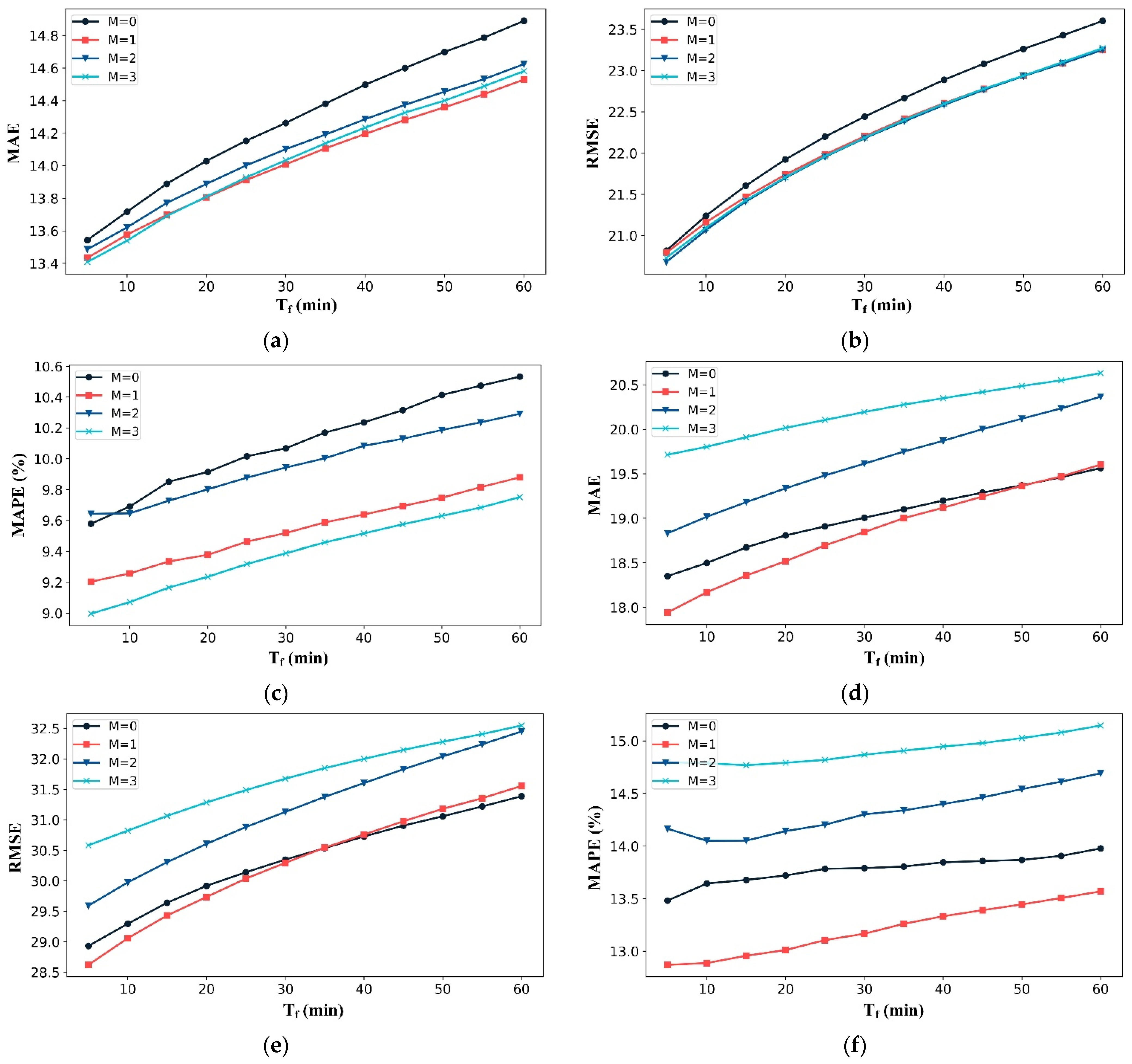
We conducted a comparative analysis to evaluate the effectiveness of the FE and STCN modules. As shown in Figure 5a–c, the black curve is the proposed F-GCN testing on the PeMSD8 datasets without the FE module (M = 0). Then, the experiment increases the order of the FE module and evaluates the performance for short-term and long-term predictions. The results indicate that the FE module model had a significantly improved effect on prediction accuracy. Specifically, when M = 3, the performance in terms of RMSE and MAPE was the best.
As shown in Figure 5d–f, the experiments on the PeMSD4 show the best performance in terms of MSE and MAPE while M = 1. Specifically, in term of RMSE, the setting with M = 3 tends to have the best performance when the forecast time T f is less than 20 min, and the setting with M = 1 has the best performance when the prediction time is greater than 20 min. Generally, M is set as one for different requirements in various application scenes. In this work, the parameter was set with M = 1 on the FE module for this dataset.
To further illustrate periodicity learning, the learning capacity of the PE module in F-GCN was evaluated on these two datasets. As shown in Figure 1, the original traffic flow fluctuates with erratic volatility, which makes it hard to extract the periodicity from them. The PE module in this work is proposed to learn this periodicity from massive traffic flow data. After the original traffic flow data were inputted into the FE module, the results were visualized as heatmaps, as shown in Figure 6, in which time ranges of 84 prediction data are displayed on PeMSD8 and PeMSD4.
As shown in Figure 6a,b from the PeMSD8 and Figure 6c,d from the PeMSD4, the output of the FE module in F-GCN presents regular periodicity. According to the color of the heat map, the traffic flow of several roads in red box 1 in Figure 6a has the same pattern because the colors are similar, but there is a significant difference between red box 1 and the red box 2, indicating that the FE module can capture differential characteristics of different roads. In black box 3, the periodicity of different roads is different in periods 36–48 and 48–60, indicating that the FE module can capture the various periodicities of the roads. The periodic fluctuation proves the effectiveness of the FE module. Then, these periodicity embeddings are transmitted to the downstream network for volatility learning.
Besides periodicity, F-GCN aims to capture volatility for traffic flow prediction from massive data. The predicted results were checked against actual traffic flow to analyze the prediction performance for volatility.
The comparison between actual traffic flow and its prediction shows that the F-GCN model could effectively capture and predict the volatility of traffic flow data. The experiment selected two typical scenes of traffic flow and visualized the comparison as shown in Figure 7. The red circles in Figure 7a,b indicate that the volatility of traffic flow is sharp, and the green circles in Figure 7c,d show a relatively flat fluctuation. The prediction from F-GCN shows good fitting in these two typical situations, which indicates that the method efficiently learns and predicts dynamic temporal volatility from the massive traffic flow.
Finally, the efficiency and accuracy of F-GCN were further evaluated with different orders of the Chebyshev polynomial. It is noteworthy that the order of the Chebyshev polynomial is different from the order of Fourier series polynomials. As listed in Table 2, training time consumption grows as the polynomial order increases. However, the overall prediction accuracy of the model tended to be the best when the order of the Chebyshev polynomial equaled 3.

5. Conclusions

In this work, a Fourier Graph Convolution Network (F-GCN) model is proposed to improve traffic flow prediction, which consists of a Fourier Embedding (FE) module and a stackable Spatial-Temporal ChebyNet (STCN) layer. The FE module was developed to learn periodicities embedding, and the stackable STCN module was integrated to learn the dynamic temporal volatility from massive traffic flow data. Extensive experiments for 15, 30, 45, and 60 min traffic flow prediction were conducted on two actual datasets, and the results indicate that the proposed F-GCN outperformed state-of-the-art methods significantly. Furthermore, the FE and STCN modules could be integrated with other deep-learning models to improve time-series analysis and prediction accuracy. In the future, the optimal order of the FE module should be explored (e.g., via Bayesian optimization) and discussed for various application scenarios.

Author Contributions

Conceptualization, L.L.; Methodology, Z.H. and C.-Y.H.; Validation, L.L., C.-Y.H. and J.S.; Formal analysis, L.L.; Data curation, Z.H.; Writing—original draft, Z.H.; Supervision, C.-Y.H.; Funding acquisition, L.L. All authors have read and agreed to the published version of the manuscript.

Funding

This work was supported in part by the projects of the National Natural Science Foundation of China (41971340, 61304199), projects of Fujian Provincial Department of Science and Technology (2021Y4019, 2020D002, 2020L3014, 2019I0019, 2008Y3001), projects of Fujian Provincial Department of Finance (GY-Z230007), and the project of Fujian Provincial Universities Engineering Research Center for Intelligent Driving Technology (Fujian University of Technology) (KF-J21012).

Data Availability Statement

The original highway datasets are derived from [11], and further raw data used in this work can be obtained from the corresponding author upon request.

Conflicts of Interest

The authors declare no conflict of interest.

Nomenclatures

AGCRNAdaptive Graph Convolutional Recurrent Network
ASTGCNAttention-based Spatial-Temporal Graph Convolution Network
ARCHAutoregressive Conditional Heteroskedasticity
ARIMAAutoregressive Integrated Moving Average
BVBoundedly Varied
CFSComplex Fourier Series
CNNConvolution Neural Networks
DCDirichlet Condition
DGCNDynamic Graph Convolution Network
EMDEmpirical Mode Decomposition
EEMDEnsemble Empirical Mode Decomposition
ELMExtreme Learning Machine
FEFourier Embedding
F-GCNFourier Graph Convolution Network
GRUGated Recurrent Unit networks
GCNGraph Convolution Network
HAHistorical Average
iGCGCNimproved Dynamic Chebyshev Graph Convolution Network
ITSIntelligent Transportation Systems
MAEMean Absolute Error
MAPEMean Absolute Percentage Error
MSEMean Square Error
PeMSPerformance Measurement System
RFSReal Fourier series
RMSERoot Mean Square Error
SPSignal Processing
STCNSpatial-Temporal ChebyNet
STSGCNSpatial-Temporal Synchronous Graph Convolutional Networks
STGCNSpatio-Temporal Graph Convolutional Network
SVRSupport Vector Regression
T-GCNTemporal Graph Convolutional Network
TSA-SLTime-Series Analysis and Supervised-Learning
· The length of a set.
Hadamard product.
[△, ○]The concatenation of and .
σ(∙)The sigmoid function.
sin · , cos · The sine and cosine functions.
The Causal convolution operator.
The Graph convolution operator.
G A graph.
VThe set of nodes in a graph.
EThe set of edges in a graph.
AThe adjacency matrix of the graph.
DThe degree matrix of A , D = j = 0 N A i , j .
LThe Laplacian matrix L = D A .
e i , j The edge between node i and node j .
X G F × N × T The spatial-temporal graph by Data Construction.
X G F × N The spatial-temporal graph in the case of d = 1 .
X G F × N × T The output of the FE module.
X G r e s F × N × T The residual X G res = X G + X G .
X g C × N × T The output of the Fine-grained Volatility Module.
X t e m p C × N × T The output of the Temporal Volatility Module.
F The number of original characteristics.
N The nodes of the graph.
T The number of time slices of the graph.
d The length of the vector embedding.
T h , T f The length of historical data and prediction data.
M The order of the Fourier polynomial in the FE module.

References

  1. Duan, H.; Wang, G. Partial differential grey model based on control matrix and its application in short-term traffic flow prediction. Appl. Math. Model. 2023, 116, 763–785. [Google Scholar] [CrossRef]
  2. Han, Y.; Zhao, S.; Deng, H.; Jia, W. Principal graph embedding convolutional recurrent network for traffic flow prediction. Appl. Intell. 2023, 1–15. [Google Scholar] [CrossRef]
  3. Guo, K.; Hu, Y.; Qian, Z.; Sun, Y.; Gao, J.; Yin, B. Dynamic graph convolution network for traffic forecasting based on latent network of laplace matrix estimation. IEEE Trans. Intell. Transp. Syst. 2020, 23, 1009–1018. [Google Scholar] [CrossRef]
  4. Li, W.; Wang, X.; Zhang, Y.; Wu, Q. Traffic flow prediction over muti-sensor data correlation with graph convolution network. Neurocomputing 2021, 427, 50–63. [Google Scholar] [CrossRef]
  5. Xue, Y.; Tang, Y.; Xu, X.; Liang, J.; Neri, F. Multi-objective feature selection with missing data in classification. IEEE Trans. Emerg. Top. Comput. Intell. 2021, 6, 355–364. [Google Scholar] [CrossRef]
  6. Williams, B.M.; Hoel, L.A. Modeling and forecasting vehicular traffic flow as a seasonal ARIMA process: Theoretical basis and empirical results. J. Transp. Eng. 2003, 129, 664–672. [Google Scholar] [CrossRef] [Green Version]
  7. Engle, R. Risk and volatility: Econometric models and financial practice. Am. Econ. Rev. 2004, 94, 405–420. [Google Scholar] [CrossRef] [Green Version]
  8. Xue, Y.; Xue, B.; Zhang, M. Self-adaptive particle swarm optimization for large-scale feature selection in classification. ACM Trans. Knowl. Discov. Data 2019, 13, 1–27. [Google Scholar] [CrossRef]
  9. Xue, Y.; Wang, Y.; Liang, J.; Slowik, A. A self-adaptive mutation neural architecture search algorithm based on blocks. IEEE Comput. Intell. Mag. 2021, 16, 67–78. [Google Scholar] [CrossRef]
  10. Zhao, L.; Song, Y.; Zhang, C.; Liu, Y.; Wang, P.; Lin, T.; Deng, M.; Li, H. T-GCN: A Temporal Graph Convolutional Network for Traffic Prediction. IEEE Trans. Intell. Transp. Syst. 2019, 21, 3848–3858. [Google Scholar] [CrossRef] [Green Version]
  11. Guo, S.; Lin, Y.; Feng, N.; Song, C.; Wan, H. Attention based spatial-temporal graph convolutional networks for traffic flow forecasting. In Proceedings of the AAAI’19: AAAI Conference on Artificial Intelligence, Honolulu, HI, USA, 27 January–1 February 2019. [Google Scholar] [CrossRef] [Green Version]
  12. Song, C.; Lin, Y.; Guo, S.; Wan, H. Spatial-Temporal Synchronous Graph Convolutional Networks: A New Framework for Spatial-Temporal Network Data Forecasting. In Proceedings of the AAAI Conference on Artificial Intelligence, New York, NY, USA, 7–12 February 2020. [Google Scholar] [CrossRef]
  13. Liao, L.; Hu, Z.; Zheng, Y.; Bi, S.; Zou, F.; Qiu, H.; Zhang, M. An improved dynamic Chebyshev graph convolution network for traffic flow prediction with spatial-temporal attention. Appl. Intell. 2022, 52, 16104–16116. [Google Scholar] [CrossRef]
  14. Chen, L.; Zheng, L.; Yang, J.; Xia, D.; Liu, W. Short-term traffic flow prediction: From the perspective of traffic flow decomposition. Neurocomputing 2020, 413, 444–456. [Google Scholar] [CrossRef]
  15. Zhang, Y.; Zhang, Y.; Haghani, A. A hybrid short-term traffic flow forecasting method based on spectral analysis and statistical volatility model. Transp. Res. Part C Emerg. Technol. 2014, 43, 65–78. [Google Scholar] [CrossRef]
  16. Chen, X.; Lu, J.; Zhao, J.; Qu, Z.; Yang, Y.; Xian, J. Traffic flow prediction at varied time scales via ensemble empirical mode decomposition and artificial neural network. Sustainability 2020, 12, 3678. [Google Scholar] [CrossRef]
  17. Tian, Z. Approach for short-term traffic flow prediction based on empirical mode decomposition and combination model fusion. IEEE Trans. Intell. Transp. Syst. 2020, 22, 5566–5576. [Google Scholar] [CrossRef]
  18. Zivot, E.; Wang, J. Vector autoregressive models for multivariate time series. Model. Financ. Time Ser. S-Plus® 2006, 385–429. [Google Scholar] [CrossRef]
  19. Sun, S.; Zhang, C.; Yu, G. A bayesian network approach to traffic flow forecasting. IEEE Trans. Intell. Transp. Syst. 2006, 7, 124–132. [Google Scholar] [CrossRef]
  20. Liu, L.; Zhen, J.; Li, G.; Zhan, G.; He, Z.; Du, B.; Lin, L. Dynamic spatial-temporal representation learning for traffic flow prediction. IEEE Trans. Intell. Transp. Syst. 2020, 22, 7169–7183. [Google Scholar] [CrossRef]
  21. Shu, W.; Cai, K.; Xiong, N.N. A Short-Term Traffic Flow Prediction Model Based on an Improved Gate Recurrent Unit Neural Network. IEEE Trans. Intell. Transp. Syst. 2021, 23, 16654–16665. [Google Scholar] [CrossRef]
  22. Guo, S.; Lin, Y.; Li, S.; Chen, Z.; Wan, H. Deep spatial–temporal 3D convolutional neural networks for traffic data forecasting. IEEE Trans. Intell. Transp. Syst. 2019, 20, 3913–3926. [Google Scholar] [CrossRef]
  23. Bruna, J.; Zaremba, W.; Szlam, A.; LeCun, Y. Spectral networks and locally connected networks on graphs. arXiv 2013, arXiv:1312.6203. [Google Scholar] [CrossRef]
  24. Defferrard, M.; Bresson, X.; Vandergheynst, P. Convolutional neural networks on graphs with fast localized spectral filtering. Adv. Neural Inf. Process. Syst. 2016, 29. [Google Scholar] [CrossRef]
  25. Kipf, T.N.; Welling, M. Semi-supervised classification with graph convolutional networks. arXiv 2016, arXiv:1609.02907. [Google Scholar] [CrossRef]
  26. Kearnes, S.; McCloskey, K.; Berndl, M.; Pande, V.; Riley, P. Molecular graph convolutions: Moving beyond fingerprints. J. Comput.-Aided Mol. Des. 2016, 30, 595–608. [Google Scholar] [CrossRef] [Green Version]
  27. Niepert, M.; Ahmed, M.; Kutzkov, K. Learning convolutional neural networks for graphs. arXiv 2016, arXiv:1605.05273. [Google Scholar] [CrossRef]
  28. Hamilton, W.L.; Ying, R.; Leskovec, J. Inductive representation learning on large graphs. Adv. Neural Inf. Process. Syst. 2017, 30. [Google Scholar] [CrossRef]
  29. Chen, C.; Li, K.; Teo, S.G.; Zou, X.; Wang, K.; Wang, J.; Zeng, Z. Gated residual recurrent graph neural networks for traffic prediction. In Proceedings of the AAAI Conference on Artificial Intelligence, Honolulu, HI, USA, 27 January–1 February 2019. [Google Scholar] [CrossRef] [Green Version]
  30. Bai, L.; Yao, L.; Li, C.; Wang, X.; Wang, C. Adaptive graph convolutional recurrent network for traffic forecasting. arXiv 2020, arXiv:2007.02842. [Google Scholar] [CrossRef]
  31. Kazemi, S.M.; Goel, R.; Eghbali, S.; Ramanan, J.; Sahota, J.; Thakur, S.; Wu, S.; Smyth, C.; Poupart, P.; Brubaker, M. Time2vec: Learning a vector representation of time. arXiv 2019, arXiv:1907.05321. [Google Scholar] [CrossRef]
  32. Meyer, F.; van der Merwe, B.; Coetsee, D.J.J.U.C.S. Learning Concept Embeddings from Temporal Data. J. Univers. Comput. Sci. 2018, 24, 1378–1402. [Google Scholar] [CrossRef]
  33. Hsu, C.-Y.; Huang, H.-Y.; Lee, L.-T. An interactive procedure to preserve the desired edges during the image processing of noise reduction. EURASIP J. Adv. Signal Process. 2010, 2010, 923748. [Google Scholar] [CrossRef] [Green Version]
  34. He, K.; Zhang, X.; Ren, S.; Sun, J. Deep residual learning for image recognition. In Proceedings of the IEEE Conference on Computer Vision and Pattern Recognition, Las Vegas, NV, USA, 27–30 June 2016. [Google Scholar] [CrossRef]
  35. Vaswani, A.; Shazeer, N.; Parmar, N.; Uszkoreit, J.; Jones, L.; Gomez, A.N.; Kaiser, Ł.; Polosukhin, I. Attention is all you need. Adv. Neural Inf. Process. Syst. 2017, 30. [Google Scholar] [CrossRef]
  36. Xue, Y.; Qin, J. Partial connection based on channel attention for differentiable neural architecture search. IEEE Trans. Ind. Inform. 2022, 1–10. [Google Scholar] [CrossRef]
  37. Chen, C.; Petty, K.; Skabardonis, A.; Varaiya, P.; Jia, Z. Freeway performance measurement system: Mining loop detector data. Transp. Res. Rec. 2001, 1748, 96–102. [Google Scholar] [CrossRef] [Green Version]
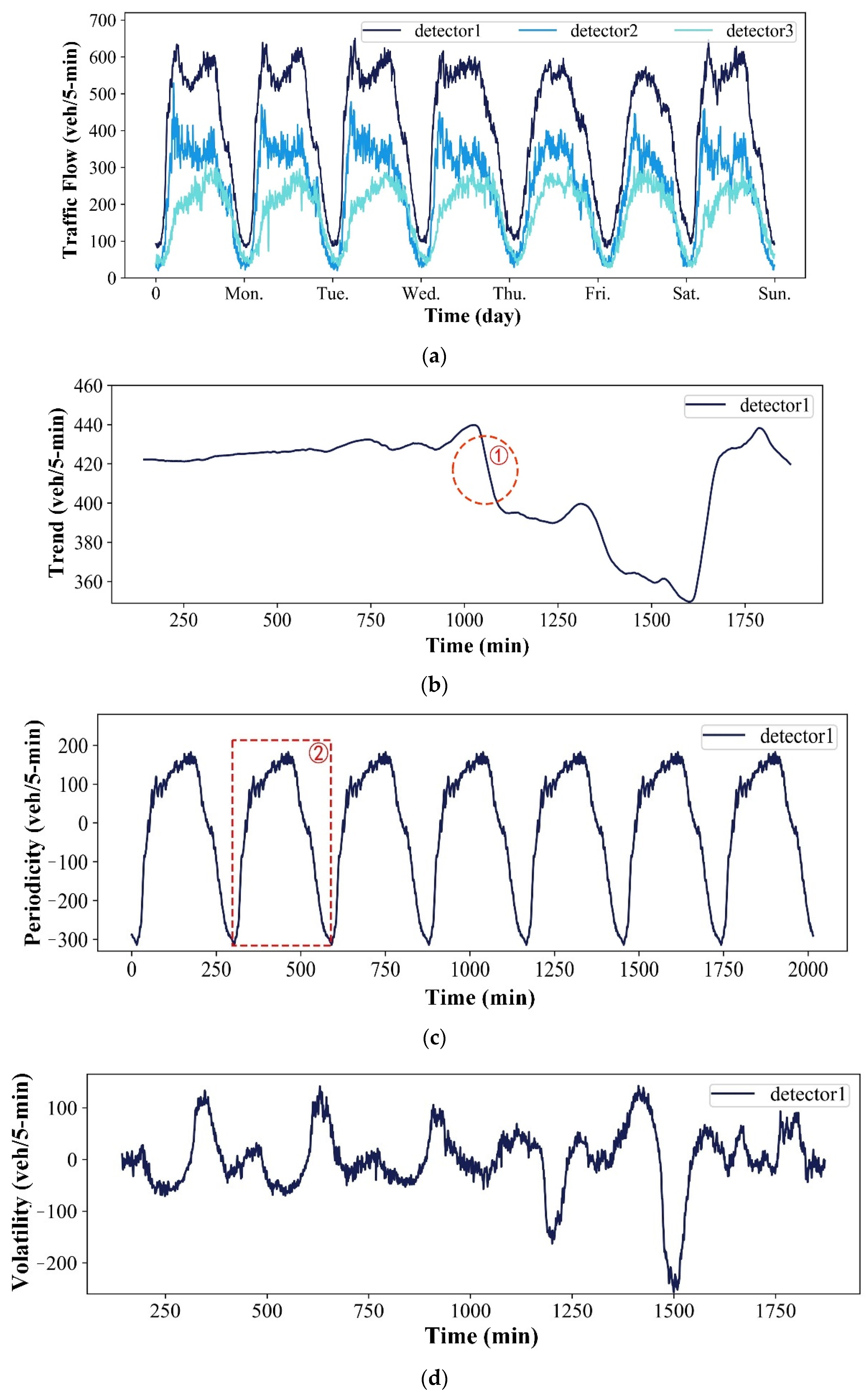
Figure 1. The sample detector’s traffic flow data [11] in one week. (a) Original data of three detectors. (bd) Three components (trend, periodicity, volatility) that are decomposed from the data of a sample. Trend and periodicity are marked with red dotted lines respectively.
Mathematics 11 01649 g001
Figure 2. The Gibbs phenomenon in the truncated Fourier series representation of the sawtooth wave function. N represents the number of harmonics.
Mathematics 11 01649 g002
Figure 3. Framework of the proposed F-GCN. F-GCN contains the data construction module, Fourier Embedding module, a STCN (stackable Spatial-Temporal ChebyNet) layer including an FVM (Fine-grained Volatility Module) and a TVM (Temporal Volatility Module), and a loss function calculation module.
Mathematics 11 01649 g003
Figure 4. Flowchart of the data construction module. The road network is represented as a graph, and the Laplacian matrix is calculated for the graph. Instead of considering all the graphs in the time dimension, predicting a target graph is based on three types of periodic data: week-period, day-period, and recent-period.
Mathematics 11 01649 g004
Figure 5. Performance of the Fourier Embedding module with a different order (M) on three indicators (MAE, RMSE, and MAPE). T f represents the time of prediction. (ac) testing on the PeMSD8 datasets, and (df) testing on the PeMSD4 datasets.
Mathematics 11 01649 g005
Figure 6. Heatmap of the output from FE module on two datasets (a,b) from the PeMSD8 datasets, and (c,d) from the PeMSD4. ① and ② represent different patterns for different roads, and ③ shows different patterns for all roads at different periods.
Mathematics 11 01649 g006
Figure 7. Comparison between actual traffic flow volatility (Ground True) and predicted results (F-GCN) of one-day data captured by detectors on four roads with node ID (a) 4 (b) 4 (c) 5, and (d) 9. Red and green circles represent steep and flat traffic flow fluctuations, respectively.
Mathematics 11 01649 g007
Table 1. Performance of the proposed model and baselines of three indicators (the best performance is highlighted in bold).
ModelsHAARIMAGRUSTGCNASTGCNSTSGCNAGCRNF-GCN
DatasetsTimeMetrics
PeMSD415 minMAE30.50528.36624.24021.19120.44820.01918.85018.358
RMSE41.87336.44336.45833.23532.07231.92730.97029.429
MAPE27.04347.37519.56118.92115.21013.53012.53612.956
30 minMAE37.24534.45525.73223.90920.73521.54319.52018.844
RMSE50.05445.59538.67135.74332.78034.18032.13030.292
MAPE36.64850.31620.87920.46515.14614.32012.96213.166
45 minMAE43.93042.04227.43325.72721.04823.05320.04019.244
RMSE58.10159.31141.14938.36233.45336.39033.10030.975
MAPE(%)53.50251.07122.55322.19315.21615.26013.31013.390
60 minMAE50.53952.99729.40827.61721.49424.62720.96019.603
RMSE65.98277.38044.01741.07734.24738.56334.42031.555
MAPE(%)72.04054.23024.70124.05415.50016.41013.88913.569
PeMSD815 minMAE25.15732.57119.20617.54216.77916.59915.08013.646
RMSE34.23434.12029.76425.87124.94125.37123.73021.384
MAPE(%)16.05322.63413.62913.08011.88810.9899.6509.424
30 minMAE30.94538.31020.45218.77417.06917.84916.09014.013
RMSE41.13043.40231.68728.03825.60027.28025.57022.171
MAPE(%)20.43830.26015.04813.91711.84211.56610.1839.634
45 minMAE36.68942.83021.92820.04017.38718.90316.96014.269
RMSE47.83647.15833.81830.15026.25728.93326.95022.742
MAPE(%)25.16335.44416.79914.86711.93312.20010.7369.792
60 minMAE42.36442.86023.67521.36217.87420.11618.17014.516
RMSE54.37945.81036.33332.22327.08830.64228.71023.230
MAPE(%)30.23635.49518.98615.92312.21013.04011.5149.924
Table 2. Time and efficiency for different orders of Chebyshev polynomial.
DatasetOrderMAERMSEMAPEs/Epoch
PeMSD8214.1422.299.8252.59
314.0222.209.5456.71
414.2922.429.7659.92
514.0322.269.6966.62
PeMSD4218.9830.3614.2793.06
318.8630.2913.21104.17
420.4232.4914.79107.97
519.6031.1113.63116.93
Disclaimer/Publisher’s Note: The statements, opinions and data contained in all publications are solely those of the individual author(s) and contributor(s) and not of MDPI and/or the editor(s). MDPI and/or the editor(s) disclaim responsibility for any injury to people or property resulting from any ideas, methods, instructions or products referred to in the content.