Development of Grey Machine Learning Models for Forecasting of Energy Consumption, Carbon Emission and Energy Generation for the Sustainable Development of Society

Abstract

Energy is an important denominator for evaluating the development of any country. Energy consumption, energy production and steps towards obtaining green energy are important factors for sustainable development. With the advent of forecasting technologies, these factors can be accessed earlier, and the planning path for sustainable development can be chalked out. Forecasting technologies pertaining to grey systems are in the spotlight due to the fact that they do not require many data points. In this work, an optimized model with grey machine learning architecture of a polynomial realization was employed to predict power generation, power consumption and CO${}_2$ emissions. A nonlinear kernel was taken and optimized with a recently published algorithm, the augmented crow search algorithm (ACSA), for prediction. It was found that as compared to conventional grey models, the proposed framework yields better results in terms of accuracy.

1. Introduction

Accurate estimation of energy generation, energy consumption and greenhouse gas emissions can determine a path for sustainable development of any country. Out of these three factors, two factors are generally monotonically increasing functions, i.e., (generation and consumption). Additionally, these are sometimes nonlinear functions that depend upon several conditions, such as political decisions, consumer-oriented policy, demand-based programs and energy conservation policies. In such a case, forecasting of these parameters becomes quite crucial. First, the non-linearity plays a crucial role, and secondly, limited data availability becomes a hurdle in the prediction.

The systems having such partial known characteristics are characterized as grey systems [1]. These systems are difficult to model and sometimes yield pretty erroneous results. Hence, during the last two decades, the research has focused on the development of a robust framework for grey architecture. In reference [2], a novel Bernoulli grey model was presented for forecasting the consumption of renewable energy. Another very interesting approach pertaining to the forecasting of renewable energy consumption has been showcased in the reference [3]. The latest research showcases the prediction of energy price with cubic polynomial realization [4]. In this work, the authors provided a cubic polynomial-based realization for market-clearing price prediction. Another important study integrating metaheuristics and grey mathematics was reported in reference [5]. The research showcased an amalgamation of a metaheuristic algorithm for parameter optimization of a whitening equation for market-clearing price prediction. The research focused on the fact that the accuracy of prediction engines can be enhanced with the applications of optimization. Applications of some optimized devices have also been investigated in the work [6]. Likewise, for modeling of carbon dioxide emissions, different intelligent methods are discussed in reference [7]. Optimization approaches require statistical comparisons; hence, a novel approach has been addressed in reference [8]. This model employs an extended deep statistical comparison to compare the optimization performance of metaheuristics. A novel adaptive structure has been implemented in reference [9] for prediction of crude oil production in China. The approach employed a fractional-order grey model along with grey wolf optimization (GWO) for implementation. Reference [10] employed the concept of weighted fractional accumulation generation in the prediction of natural gas production. The authors employed five distinct nature inspired optimization algorithms in this work. A seasonal variation index has been proposed for consumption of the residential electricity consumption. The authors claimed that this integration can bring speed to forecasting [11]. An application of the cuckoo search for forecasting the consumer demand in the New South Wales area was conducted in reference [12]. In this work, a single parameter was optimized by the algorithm. Another very interesting approach with this algorithm can be seen in reference [13]. The algorithm was employed to predict thermal error compensation for CNC machine tools.

It is also worth mentioning here that integration of a grey architecture with optimization algorithms for tuning the parameters is also a potential area of research. In reference [14], a rolling grey model was proposed for economic prediction with the help particle swarm optimization (PSO). It is worth mentioning here that PSO is still the most suitable algorithm for nonlinear functions. Further, in reference [15], a very interesting prediction was executed for sales and stock piling of electric vehicles using an adaptive optimized grey model. From these approaches, it is evident that research is aggregating towards the adaptive and optimized model as compared to rigid, fixed-structure grey models. The inverse square reverse unit (ISRU) activation function has been integrated with the grey model to forecast power consumption in China. This function helps to explain data growth, and this yields high accuracy in the predictions [16]. Likewise, an integration of the grasshopper optimization algorithm (GOA) and the time-delayed grey model has been presented in reference [17], and its applications in the prediction have been reported prominently.

On the basis of this discussion, the following research objectives are framed. The outcomes of this research were evaluated with the help of the framework proposed to reach these objectives.

• To discuss the mathematical framework of the proposed nonlinear-kernel-based implementation and develop an optimization routine for estimating parameters of the nonlinear whitening equation.
• To assure applicability of this realization for the prediction of energy generation, consumer demand, and forecasting of CO${}_2$ emissions.
• To employ the augmented crow search algorithm (ACSA) for optimizing the parameters of this framework and evaluate the framework by the calculation of various error indices, such as absolute percentage error and the mean of this error.

The remaining part of the paper is organized as follows. Section 2 presents a development model of OFOPGM and mathematical details of the naïve grey model. Section 3 showcases the optimization capabilities of the augmented crow search algorithm and establishes the efficacy and implementation details of the ACSA for the parameter-estimation process. Section 4 presents analysis of the results for the proposed approach and comparative analysis with other conventional grey models for predictions of various parameters. Finally, all major findings are summarized in a lucid form in Section 5. Some future research directions are also chalked out with reference to our experimentation.

2. Development of a Grey Model Based on the Optimized Fractional Overhead Power Term Polynomial Grey Model (OFOPGM)

The model based on optimized whitening equation has been presented in reference [5]. The model has been employed for the prediction of the market-clearing price for energy trading. The model has been tested for various datasets of market-clearing price. The efficacy of the model for dealing with nonlinear data became a primary reason to employ it for this work.

Theorem 1.

The representative expression for time series for energy generation, energy consumption and related to CO${}_2$ emissions can be cumulatively represented by the following notation:

$$E^{\left(0\right)}=[E^{\left(0\right)}\left(1\right),E^{\left(0\right)}\left(2\right)\dots \dots E^{\left(0\right)}\left(k\right)]$$

and

$$E^{\left(1\right)}=[E^{\left(1\right)}\left(1\right),E^{\left(1\right)}\left(2\right)\dots \dots E^{\left(1\right)}\left(k\right)]$$

represents the series obtained after one time accumulation; $z^{\left(1\right)}\left(k\right)$ is the background value. The basic form of an optimized grey model is proposed as

$$\frac{d{E}^{\left(1\right)}\left(t\right)}{dt}+a{E}^{\left(1\right)}\left(t\right)=m{t}^{\alpha }+n{t}^{\beta }+d$$

(1)

where a is the development coefficient and $m{t}^{\alpha }+n{t}^{\beta }+d$ is stochastic grey action quantity. Here, α and β are design parameters, which are computed through an optimization process.

Now, the system can be represented as

$$\begin{array}{c}\hfill E^{\left(0\right)}\left(l\right)+a{z}^{\left(1\right)}\left(l\right)=\frac{m}{(\alpha +1)}\times (l^{\alpha +1}-{(l-1)}^{\alpha +1})..\\ \hfill +\frac{n}{(\beta +1)}\times (l^{\beta +1}-{(l-1)}^{\beta +1})+d\end{array}$$

(2)

Proof of Theorem 1.

The whitening equation integration between the interval $[l-1,l]$ is

$${\int }_{l-1}^{l}d{E}^{\left(1\right)}\left(t\right)dt+{\int }_{l-1}^{l}a{E}^{\left(1\right)}\left(t\right)dt={\int }_{l-1}^l\left(m{t}^{\alpha }+n{t}^{\beta }+d\right)dt$$

(3)

$$\begin{array}{c}\hfill \left[E^{\left(1\right)}\left(l\right)-E^{\left(1\right)}(l-1)\right]+a{\int }_{l-1}^l{E}^{\left(1\right)}\left(t\right)dt=\frac{m}{(\alpha +1)}\\ \hfill (l^{\alpha +1}-{(l-1)}^{\alpha +1})+\frac{n}{(\beta +1)}(l^{\beta +1}-{(l-1)}^{\beta +1})+d\end{array}$$

(4)

From the expression for inverse accumulation, the original values can be obtained from accumulated values and can be expressed as:

$$E^{\left(0\right)}\left(l\right)=E^{\left(1\right)}\left(l\right)-E^{\left(1\right)}(l-1)$$

(5)

and part of the expression (11) can be appended from trapezoidal rule application; i.e.,

$$a{\int }_{l-1}^l{E}^{\left(1\right)}\left(t\right)dt=\frac{a}{2}\times (E^{\left(1\right)}\left(l\right)+E^{\left(1\right)}(l-1))$$

(6)

by substituting the expressions from (5) and (6) in expression (4), the theorem can be proved.

$$\begin{array}{c}\hfill E^{\left(0\right)}\left(l\right)+a{z}^1\left(l\right)=\frac{m}{(\alpha +1)}\times (l^{\alpha +1}-{(l-1)}^{\alpha +1})..\\ \hfill +\frac{n}{(\beta +1)}\times (l^{\beta +1}-{(l-1)}^{\beta +1})+d\end{array}$$

(7)

 □

Theorem 2.

The parameters of whitening equation can be given by a least-square algorithm: ${(a,m,n,d)}^T=\left(B^T{B}^{-1}\right)B^{T}Y$ where

$$Y={\left[\begin{array}{ccccc}{E}^{\left(0\right)}\left(2\right)& ..& ..& ..& E^{\left(0\right)}\left(k\right)\end{array}\right]}^T$$

and B can be expressed as

$$B=\left[\begin{array}{cccc}-z^{\left(1\right)}\left(2\right)& \frac{1}{(\alpha +1)}\times (2^{(\alpha +1)}-1^{(\alpha +1)})& \frac{1}{(\beta +1)}\times (2^{(\beta +1)}-1^{(\beta +1)})& 1\\ -z^{\left(1\right)}\left(3\right)& \frac{1}{(\alpha +1)}\times (3^{(\alpha +1)}-2^{(\alpha +1)})& \frac{1}{(\beta +1)}\times (3^{(\beta +1)}-2^{(\beta +1)})& 1\\ :& :& :& :\\ :& :& :& :\\ -z^{\left(1\right)}\left(k\right)& \frac{1}{(\alpha +1)}\times (k^{(\alpha +1)}-{(k-1)}^{(\alpha +1)})& \frac{1}{(\beta +1)}\times (k^{(\beta +1)}-{(k-1)}^{(\beta +1)})& 1\end{array}\right]$$

(8)

Proof. 

By considering the expression (7), we substitute in $k=2$.

$$\begin{array}{c}\hfill M^{\left(0\right)}\left(2\right)=a\times -z^{\left(1\right)}\left(2\right)+\frac{m}{(\alpha +1)}\times (2^{(\alpha +1)}-1^{(\alpha +1)})..\\ \hfill +\frac{n}{(\beta +1)}\times (2^{(\beta +1)}-1^{(\beta +1)})+d\end{array}$$

(9)

Now by substituting with $k=j$

$$\begin{array}{c}\hfill M^{\left(0\right)}\left(j\right)=a\times -z^{\left(1\right)}\left(j\right)+\frac{b}{(\alpha +1)}\times (j^{(\alpha +1)}-{(j-1)}^{(\alpha +1)})..\\ \hfill +\frac{c}{(\beta +1)}\times (j^{(\beta +1)}-{(j-1)}^{(\beta +1)})+d\end{array}$$

(10)

With the application of mathematical induction, we can write the same expression for $k=j+1$:

$$\begin{array}{c}\hfill E^{\left(0\right)}(j+1)=a\times -z^{\left(1\right)}(j+1)\\ \hfill +\frac{m}{(\alpha +1)}\times ({(j+1)}^{(\alpha +1)}-j^{(\alpha +1)})\\ \hfill +\frac{n}{(\beta +1)}\times ({(j+1)}^{(\beta +1)}-j^{(\beta +1)})+d\end{array}$$

(11)

By converting the expressions (9)–(11), the matrix form of these equations (for $n^{th}terms$ can be obtained, and a solution of the least-square algorithm can be found.

$$\begin{array}{c}\hfill \left[\begin{array}{cccc}-z^{\left(1\right)}\left(2\right)& \frac{1}{(\alpha +1)}\times (2^{(\alpha +1)}-1^{(\alpha +1)})& \frac{1}{(\beta +1)}\times (2^{(\beta +1)}-1^{(\beta +1)})& 1\\ -z^{\left(1\right)}\left(3\right)& \frac{1}{(\alpha +1)}\times (3^{(\alpha +1)}-2^{(\alpha +1)})& \frac{1}{(\beta +1)}\times (3^{(\beta +1)}-2^{(\beta +1)})& 1\\ :& :& :& :\\ :& :& :& :\\ -z^{\left(1\right)}\left(k\right)& \frac{1}{(\alpha +1)}\times (k^{(\alpha +1)}-{(k-1)}^{(\alpha +1)})& \frac{1}{(\beta +1)}\times (k^{(\beta +1)}-{(k-1)}^{(\beta +1)})& 1\end{array}\right]\times \left[\begin{array}{c}a\\ m\\ n\\ d\end{array}\right]=\left[\begin{array}{c}{E}^{\left(0\right)}\left(2\right)\\ E^{\left(0\right)}\left(3\right)\\ :\\ :\\ E^{\left(0\right)}\left(k\right)\end{array}\right]\end{array}$$

(12)

 □

After calculating the coefficient of the whitening equation, the response of the forecaster has been evaluated with the help of the following equation.

$$\begin{array}{c}\hfill E^0\left(k\right)=E^{\left(1\right)}\left(1\right)\times e^{-a(k-1)}+\sum _{l=2}^k\frac{1}{2}\times [e^{-a(k-l)}\times (m{l}^{\alpha }+n{l}^{\beta }+d)\\ \hfill +e^{-a(k-l+1)}\times (m{(l-1)}^{\alpha }+n{(l-1)}^{\beta }+d)]-E^{\left(1\right)}\left(1\right)\times e^{-a(k-2)}\\ \hfill -\sum _{l=2}^{k-1}\frac{1}{2}\times [e^{-a(k-1-l)}\times (m{l}^{\alpha }+n{l}^{\beta }+d)\\ \hfill -e^{-a(k-l)}\times (m{(l-1)}^{\alpha }-n{(l-1)}^{\beta }+d)]\end{array}$$

(13)

Here, in this equation, the parameters $\alpha$ and $\beta$ are adaptive and computed with the help of an optimization routine. For establishing an optimized framework, let us define the error (mean absolute percentage error (MAPE)) as per the following expression:

$$\mathrm{MAPE}=\frac{1}{k}\sum _{r=1}^k\left|\frac{{\widehat{E}}^{\left(0\right)}\left(r\right)-E^{\left(0\right)}\left(r\right)}{E^{\left(0\right)}\left(r\right)}\right|\times 100$$

(14)

where ${\widehat{E}}^{\left(0\right)}\left(r\right)$ is the predicted output by the forecaster, and $E^0\left(r\right)$ is the actual value of the corresponding $s^{th}$ sample. Further the optimization routine has been established considering the cumulative values of all the samples in forecasting. In most of the forecasting approaches, the MAPE index is chosen.

$$\mathrm{J}(\alpha ,\beta )=Min(\frac{1}{k}\sum _{r=1}^k\left|\frac{{\widehat{E}}^{\left(0\right)}\left(r\right)-E^{\left(0\right)}\left(r\right)}{E^{\left(0\right)}\left(r\right)}\right|\times 100)$$

(15)

The objective function is defined as per Equation (15), where the variables are optimized with the help of an optimization algorithm and a fixed structure of whitening equation is obtained. Readers are directed to reference [5] for proof of Equation (13).

3. Augmented Crow Search Algorithm (ACSA)

Recently, a crow search algorithm has caught the eyes of researchers with its excellent convergence properties and the ability to solve complex design problems with ease [18]. Diverse applications of the algorithm have been reported in many fields. A rich survey of CSA was conducted [19] to depict the diverse applications and fields of implementation of CSA. Recently, a version of CSA has been developed that employs a sinusoidal truncated function with opposition-based learning for solving harmonic estimation problems. The method has been tested over diverse sets of harmonics, and analysis of the proposed algorithm exposed real challenges. From the observation of the author, it has been concluded that the algorithm is very useful for applications on nonlinear functions [20]. The following features of the ACSA are noteworthy for its implementation as an estimation agent for this problem (Algorithm 1):

• The author has tested the ACSA on diverse sets of nonlinear, noisy and composite functions. These functions contain exponential, trigonometric and other nonlinear terms. From this application to 40 different functions, it is evident that the algorithm is capable of handling the parameter-estimation process very efficiently.
• The ACSA employs an opposition-based algorithm for initializing the search agents. This phenomenon can be seen in many prominent algorithms. By employing opposition-based learning in this phase, the designer wishes to ensure the effective exploration. In many of the experiments, these facts have been established that with the incorporation of OBL, the performance of the algorithm is significantly enhanced [20].
• The ACSA employs a sinusoidal truncated function that restricts the algorithm search space in exploitation phase. This function provides a bridge between exploration and exploitation.

For further information about the CSA, readers are directed to the following Refs. [21,22]. The following section presents the analysis of the results for the implemented approach.

Algorithm 1 Augmented crow search algorithm.
1:	Generate an initial half of the population of size $N_p/2$ consisting of each vector with dimension $D=2$ ($\alpha ,\beta$). Remaining Half will be the opposite population.
2:	Iteration = 0
3:	while Iteration < Maximum no. of Iteration do
4:	Evaluate fitness for each crow, position and memory updation.
5:	for i = 1 to $N_p$ do
6:	Randomly choose any crow, Define Awareness probability and Flight length as per updated Cosine law.
7:	if fitness of solution < fitness of target then
8:	Trail replaces target.
9:	end if
10:	end for
11:	Update memory of the crows
12:	Iteration = Iteration + 1
13:	end while
14:	Output

4. Results

For showcasing the efficacy of the proposed non-linear framework, four case studies were chosen, and predictions were made. The following four case studies were considered.

• Case study 1—carbon dioxide emission [23]: The author of reference [23] developed a forecasting model for prediction of carbon dioxide emission in Vietnam. In addition to that, the same models were applied for prediction of the generation forecast. The analysis was performed for the years 2010–2019. Case studies 1–4 were conducted with the data of the reference.
• Case study 2—carbon dioxide emission [24]: An exponential grey forecasting model was deployed for the forecasting of carbon dioxide emissions in Taiwan during 2002 to 2012.
• Case study 3—energy generation forecast [25]: The data were taken from the reference, where a foe was developed for 5.6 kW grid-connected PV-system generation data in Beijing from 1997 to 2006. The forecast was conducted with the help of a conventional grey model, along with grey Markov models.
• Case study 4—energy consumption forecast [23]: The energy consumption data of Vietnam were taken for the analysis.

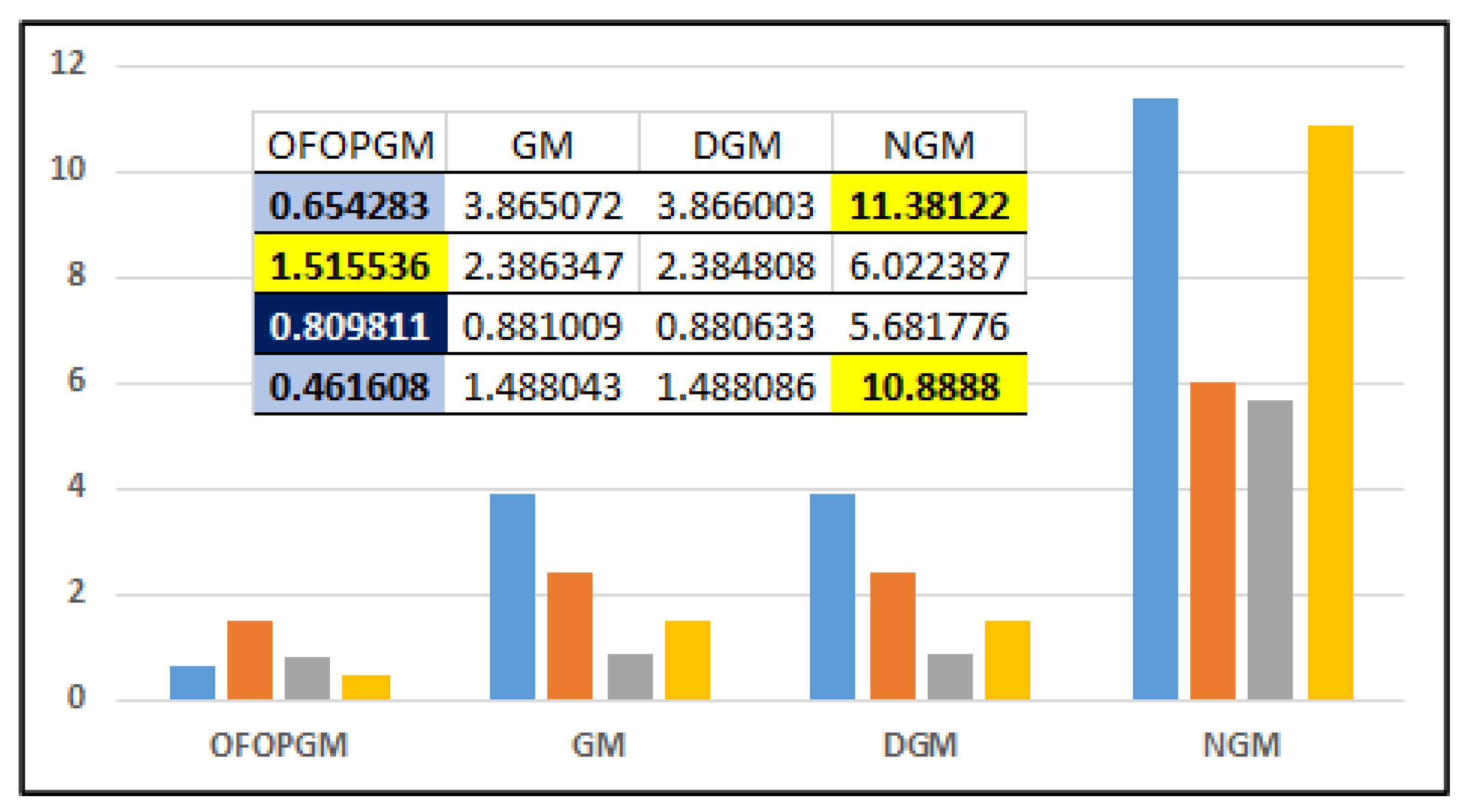
To compare the proposed framework to others, three conventional grey models were employed. The first one was a conventional grey model that was formed on the basis of research presented in reference [26]. A comparison was made with discrete and novel grey forecasting models presented in references [27,28]. The results of case study 1 are depicted in

Table 1. CO${}_2$ emission forecast [23].

Original Value	OFOPGM	Error	APE	GM	Error	APE
14,273	14,273	0	0	14,273	0	0
15,216	15,336.59	0.792528425	0.792528	14,451.25	−5.02595	5.025951
14,222	14,342.85	0.849768383	0.849768	14,946.08	5.091282	5.091282
14,723	14,848.07	0.849474876	0.849475	15,457.86	4.991216	4.991216
16,691	16,821.13	0.779644077	0.779644	15,987.16	−4.21691	4.216912
MAPE			0.654283			3.865072
	DGM	Error	APE	NGM	Error	APE
14,273	14,273	0	0	14,273	0	0
15,216	14,475.15	−4.86891695	4.868917	8499.795	−44.1391	44.1391
14,222	14,956.17	5.162214843	5.162215	13,930.95	−2.04646	2.046457
14,723	15,453.18	4.959449536	4.95945	15,019.86	2.016268	2.016268
16,691	15,966.71	−4.33943158	4.339432	15,238.17	−8.70427	8.704266
MAPE			3.866003			11.38122

, which show a case comparison of the proposed framework with the conventional grey model, DGM and NGM. When inspecting the values of error depicted in table, it is evident to say that the MAPE (0.65) is optimal for the proposed grey framework and other forecasts contain high values of errors. It is worth mentioning here that for this particular case, NGM gives very high values of error (11.38). The best values and worst values both are highlighted. The significance of the grey model is seen by the fact that when the data points were limited, it could still generate a fair forecast. From here, it can be observed that with five data values, it can generate an accurate forecast.

In addition to the MAPE values, error and absolute percentage error (APE) are also shown in the tables. From these values, it is clear that the forecast is not very far from the actual values for the proposed framework. Hence, it can be concluded that the proposed framework is able to conduct forecasts in an efficient manner.

Similar results were witnessed when case study 2 was evaluated. The prediction results of the case study are showcased in

Table 2. CO${}_2$ emission forecast 2 [24].

Original	GM(1,1)	APE	OFOPGM	APE
225.245	225.245	0	225.245	0
243.804	255.4287	4.76804	243.804	1.29 × 10${}^{-8}$
252.647	256.0806	1.359047	259.4589	2.696208
260.702	256.7342	1.521978	265.2393	1.740402
267.782	257.3894	3.880984	266.1546	0.607738
271.85	258.0463	5.077672	264.7293	2.61936
261.524	258.7049	1.077933	262.4669	0.360559
246.128	259.3652	5.378189	260.3375	5.773206
262.799	260.0272	1.054724	258.9959	1.447156
255.73	260.6909	1.939878	258.898	1.238822
260.857	261.3562	0.191369	260.368	0.187446
MAPE		2.386347		1.515536
225.245	225.245	0	225.245	0
243.804	255.4992	4.796955	147.5414	39.4836
252.647	256.1357	1.380872	233.016	7.770137
260.702	256.7739	1.506746	254.0143	2.565284
267.782	257.4136	3.871946	259.1728	3.21499
271.85	258.055	5.074504	260.4401	4.19712
261.524	258.6979	1.08063	260.7515	0.295399
246.128	259.3424	5.368925	260.8279	5.972479
262.799	259.9886	1.069423	260.8467	0.742874
255.73	260.6363	1.918554	260.8513	2.002639
260.857	261.2857	0.164336	260.8525	0.001731
MAPE		2.384808		6.022387

. Here also, the MAPE values are quite optimal for the proposed framework (1.515536). However, unlike the previous case, the performance of NGM (6.02) was not compromised much. From this, it is concluded that the performances of the grey models are quite sensitive to data characteristics. Hence, it can also be seen that to have good forecasting performance, the forecaster should be able to handle the data in a very efficient manner, like the proposed framework.

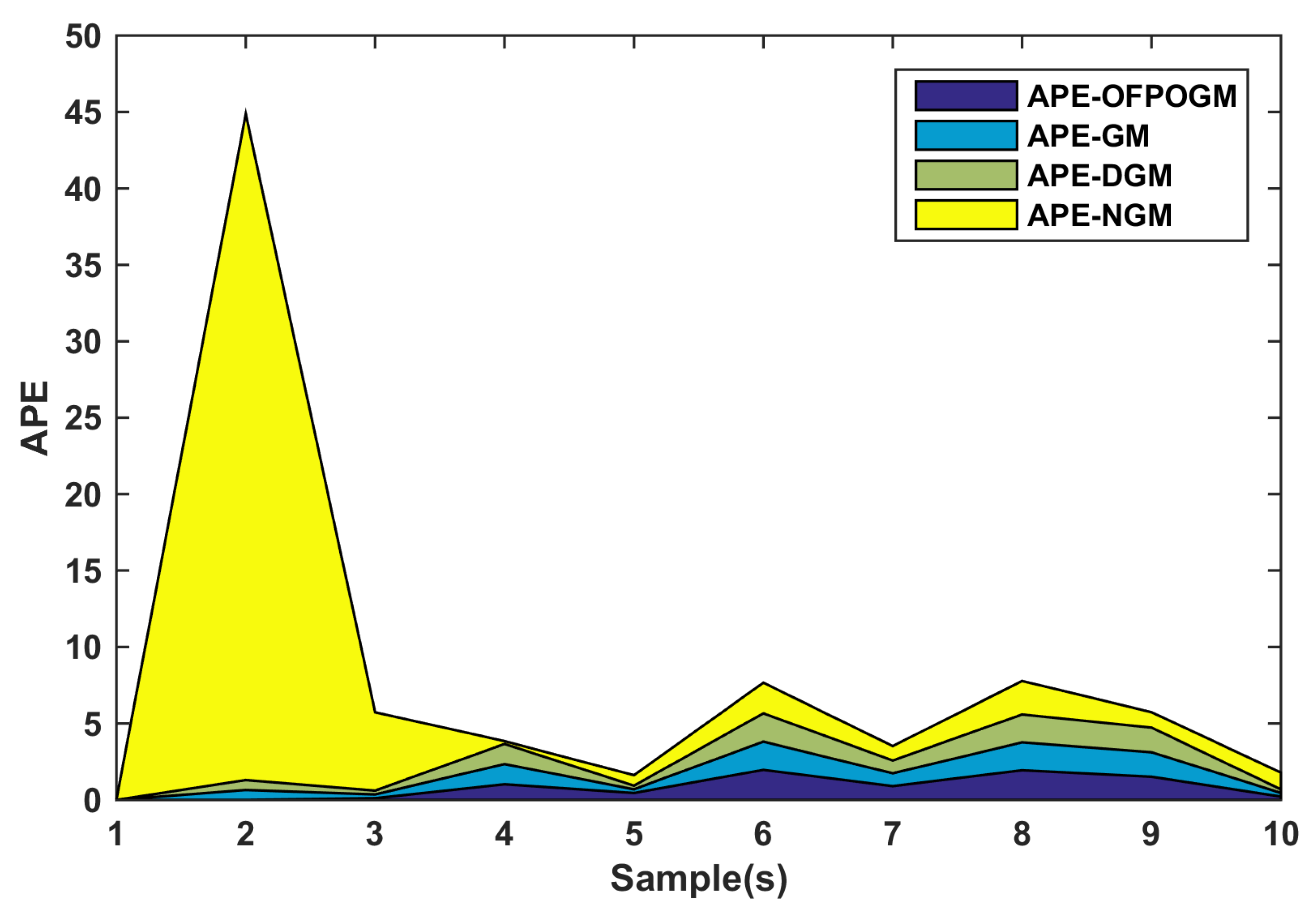
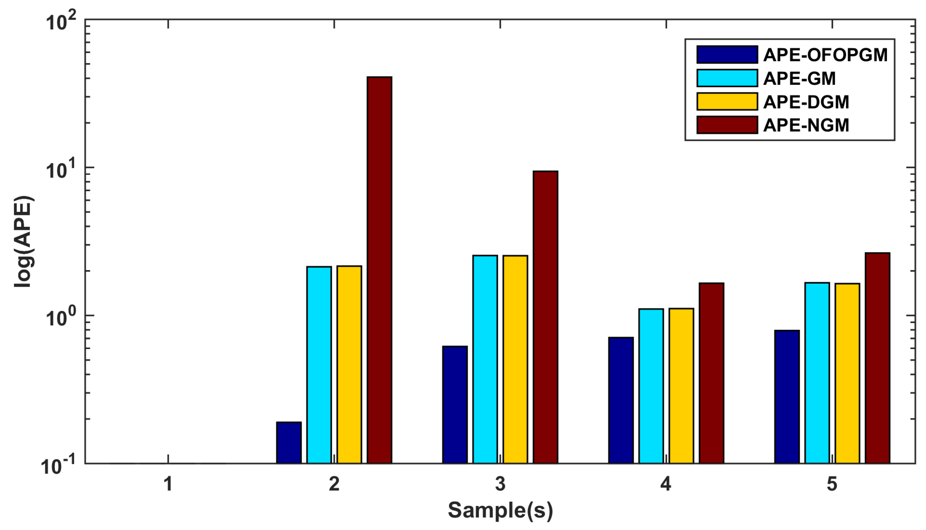
While inspecting the forecasting performance of the engine for case 3, especially for forecasting the energy generation,

Table 3. Energy Generation Forecast [25].

Year	Data	OFOPGM	Error	APE	GM	Error	APE
1997	5147.36	5147.36	0	0	5147.36	0	0
1998	5084	5084	1.41 × 10${}^{-9}$	1.41 × 10${}^{-9}$	5051.05	−0.64812	0.648117
1999	5026	5031.646	0.112213	0.112213	5038.35	0.245722	0.245722
2000	4960.26	5011.29	1.018303	1.018303	5025.68	1.318882	1.318882
2001	5024.98	5002.337	−0.45264	0.452643	5013.05	−0.23741	0.237414
2002	5094.76	4996.969	−1.95701	1.957011	5000.44	−1.85131	1.851314
2003	4946.36	4991.135	0.897098	0.897098	4987.87	0.839203	0.839203
2004	4886.02	4982.355	1.93353	1.93353	4975.33	1.827868	1.827868
2005	5043.88	4968.929	−1.50839	1.50839	4962.83	−1.6069	1.606898
2006	4938.76	4949.596	0.218925	0.218925	4950.35	0.234674	0.234674
MAPE				0.809811			0.881009
Year	Data	DGM	Error	APE	NGM	Error	APE
1997	5147.36	5147.36	0	0	5147.36	0	0
1998	5084	5051.259	−0.644	0.643999	2868.134	−43.5851	43.5851
1999	5026	5038.509	0.248879	0.248879	4768.478	−5.1238	5.123805
2000	4960.26	5025.79	1.321109	1.321109	4969.252	0.181272	0.181272
2001	5024.98	5013.104	−0.23633	0.236333	4990.464	−0.6869	0.686896
2002	5094.76	5000.45	−1.85111	1.851113	4992.705	−2.00314	2.003143
2003	4946.36	4987.828	0.838355	0.838355	4992.941	0.941732	0.941732
2004	4886.02	4975.238	1.825981	1.825981	4992.966	2.188826	2.188826
2005	5043.88	4962.679	−1.60989	1.609886	4992.969	−1.00936	1.00936
2006	4938.76	4950.152	0.230674	0.230674	4992.969	1.097632	1.097632
MAPE				0.880633			5.681776

shows the obtained results. The pictorial representation of APE is showcased with the help of Figure 1. The x axis of the figure showcases the no. of datapoints, and on the y axis, the APE is shown. It can be observed that again, the NGM gives pessimistic results, but the proposed framework outperforms the other model, achieving high accuracy. Hence, it is concluded that the proposed optimal framework is meaningful, and it can conduct forecasts with higher accuracy. Further, similar results were obtained for case 4. The results are depicted with the help of

Table 4. Energy consumption forecast [23].

Original	OFOPGM	Error	APE	GM	Error	APE
3479	3479	0	0	3479	0	0
3652	3658.935	0.18989855	0.189899	3729.86	2.131988	2.131988
3810	3833.542	0.617903739	0.617904	3713.234	−2.53978	2.539784
3738	3764.506	0.709090175	0.70909	3696.682	−1.10534	1.105341
3620	3648.64	0.791146875	0.791147	3680.204	1.663101	1.663101
MAPE			0.461608	1.488043
Original	DGM	Error	APE	NGM	Error	APE
3479	3479	0	0	3479	0	0
3652	3730.692	2.154761975	2.154762	2164.233	−40.7384	40.73841
3810	3713.51	−2.53254274	2.532543	3451.338	−9.41371	9.413708
3738	3696.407	−1.11269483	1.112695	3676.288	−1.65094	1.650936
3620	3679.384	1.640430373	1.64043	3715.603	2.640969	2.640969
MAPE			1.488086	10.8888

and Figure 2. The x axis of the figure showcases the no. of datapoints, and on the y axis, the APE is shown.

5. Discussion

The pictorial representation of the MAPE values is shown in Figure 3. From this figure, it is evident that the MAPE values are optimal for the proposed model. Additionally, it can be concluded that the NGM model provides pessimistic results, and the scope for improvement in the forecasting performance is there. Additionally, with a slight change in the whitening equation, grey models can be applicable for this prediction. Hence, it is concluded that the proposed optimized framework can be employed for the design and planning of a town.

Further, the results of optimization process handled by the ACSA have been showcased in terms of $\alpha$ and $\beta$ values (

Table 5. Polynomial coefficients generated by the ACSA.

Parameter/Cases	$\mathit{\alpha }$	$\mathit{\beta }$
Case-1	2.1011	0.8822
Case-2	3.2674	0.6822
Case-3	2.2576	0.1512
Case-4	3.2649	0.1499

). While using these parameters, one can easily obtain the whitening equation. For all cases, these values of parameters were obtained, and the forecast was calculated. It can be observed that with the help of the ACSA, the parameter-estimation process can be easily handled, and that too with higher accuracy as compared with other conventional models of the grey systems.

6. Conclusions

The paper addresses an important issue of forecasting of energy consumption, energy generation and carbon emission forecasting. We proposed an optimized framework based on a nonlinear polynomial-based machine learning kernel for prediction of these three parameters. The structure of this polynomial was optimized with the application of the ACSA. Three different case studies of forecasting were accomplished by implementing this optimized framework. The following are the major outcomes of this study:

• An optimized framework for forecasting of a grey system was evaluated, and the mathematical foundation of the work has been exhibited. While presenting this framework, the implication of the correctness of polynomial coefficients was also demonstrated.
• Three case studies were performed for evaluating the performance of this kernel-based implementation. The case studies are related to forecasting of the energy generation, energy consumption and carbon dioxide gas emission. It was found that the proposed architecture yields a good performance on these datasets when compared with other conventional models.
• The evaluation of the framework was performed through the use of error indices called APE and mean absolute percentage error (MAPE). It was observed that the MAPE of the optimized model is optimal when compared with those of other models. The accurate estimation of these parameters would be quite helpful for planners of energy grids and towns.
• It is worth mentioning here that while evaluating the forecaster’s performance, the Lewis criterion was employed. As mentioned in reference [29] and according to criterion of Lewis, the MAPE obtained from the proposed framework fell in a fair range for each case study. Hence, it can be concluded that optimization handled with the help of the ACSA yields an optimal architecture for the whitening equation of the model, and it exhibited fair performance.

Further, the application of this model will be evaluated with the application of different metaheuristics and on more challenging time-series prediction problems.

References

1. Liu, S.; Forrest, J.Y.L. Grey Systems: Theory and Applications; Springer Science & Business Media: Berlin/Heidelberg, Germany, 2010. [Google Scholar]
2. Duan, H.; Wang, S.; He, C.; Huang, J. Application of a novel grey Bernoulli model to predict the global consumption of renewable energy. Energy Rep. 2021, 7, 7200–7211. [Google Scholar] [CrossRef]
3. Tsai, S.B. Using grey models for forecasting China’s growth trends in renewable energy consumption. Clean Technol. Environ. Policy 2016, 18, 563–571. [Google Scholar] [CrossRef]
4. Saxena, A.; Alrasheedi, A.F.; Alnowibet, K.A.; Alshamrani, A.M.; Shekhawat, S.; Mohamed, A.W. Local Grey Predictor Based on Cubic Polynomial Realization for Market Clearing Price Prediction. Axioms 2022, 11, 627. [Google Scholar] [CrossRef]
5. Saxena, A. Optimized Fractional Overhead Power Term Polynomial Grey Model (OFOPGM) for market clearing price prediction. Electr. Power Syst. Res. 2023, 214, 108800. [Google Scholar] [CrossRef]
6. Sharma, A.K.; Saxena, A.; Tiwari, R. Optimal placement of svc incorporating installation cost. Int. J. Hybrid Inf. Technol. 2016, 9, 289–302. [Google Scholar] [CrossRef]
7. Assad, M.E.H.; Mahariq, I.; Al Barakeh, Z.; Khasawneh, M.; Amooie, M.A. Modeling CO2 emission of Middle Eastern countries using intelligent methods. Comput. Mater. Contin. 2021, 69, 3767–3781. [Google Scholar]
8. Eftimov, T.; Korošec, P. A novel statistical approach for comparing meta-heuristic stochastic optimization algorithms according to the distribution of solutions in the search space. Inf. Sci. 2019, 489, 255–273. [Google Scholar] [CrossRef]
9. Wang, Y.; Ye, L.; Yang, Z.; Ma, X.; Wu, W.; Wang, L.; Luo, Y. A novel structure adaptive fractional discrete grey forecasting model and its application in China’s crude oil production prediction. Expert Syst. Appl. 2022, 207, 118104. [Google Scholar] [CrossRef]
10. Liu, C.; Lao, T.; Wu, W.Z.; Xie, W.; Zhu, H. An optimized nonlinear grey Bernoulli prediction model and its application in natural gas production. Expert Syst. Appl. 2022, 194, 116448. [Google Scholar] [CrossRef]
11. Xiong, X.; Hu, X.; Guo, H. A hybrid optimized grey seasonal variation index model improved by whale optimization algorithm for forecasting the residential electricity consumption. Energy 2021, 234, 121127. [Google Scholar] [CrossRef]
12. Jiang, P.; Zhou, Q.; Jiang, H.; Dong, Y. An optimized forecasting approach based on grey theory and Cuckoo search algorithm: A case study for electricity consumption in New South Wales. Abstr. Appl. Anal. 2014, 2014, 183095. [Google Scholar] [CrossRef] [Green Version]
13. Abdulshahed, A.M.; Longstaff, A.P.; Fletcher, S. A cuckoo search optimisation-based Grey prediction model for thermal error compensation on CNC machine tools. Grey Syst. Theory Appl. 2017, 7, 146–155. [Google Scholar] [CrossRef] [Green Version]
14. Liu, L.; Wang, Q.; Wang, J.; Liu, M. A rolling grey model optimized by particle swarm optimization in economic prediction. Comput. Intell. 2016, 32, 391–419. [Google Scholar] [CrossRef]
15. Ding, S.; Li, R. Forecasting the sales and stock of electric vehicles using a novel self-adaptive optimized grey model. Eng. Appl. Artif. Intell. 2021, 100, 104148. [Google Scholar] [CrossRef]
16. Huang, L.; Liao, Q.; Zhang, H.; Jiang, M.; Yan, J.; Liang, Y. Forecasting power consumption with an activation function combined grey model: A case study of China. Int. J. Electr. Power Energy Syst. 2021, 130, 106977. [Google Scholar] [CrossRef]
17. Xiang, X.; Ma, X.; Fang, Y.; Wu, W.; Zhang, G. A novel hyperbolic time-delayed grey model with Grasshopper Optimization Algorithm and its applications. Ain Shams Eng. J. 2021, 12, 865–874. [Google Scholar] [CrossRef]
18. Askarzadeh, A. A novel metaheuristic method for solving constrained engineering optimization problems: Crow search algorithm. Comput. Struct. 2016, 169, 1–12. [Google Scholar] [CrossRef]
19. Hussien, A.G.; Amin, M.; Wang, M.; Liang, G.; Alsanad, A.; Gumaei, A.; Chen, H. Crow search algorithm: Theory, recent advances, and applications. IEEE Access 2020, 8, 173548–173565. [Google Scholar] [CrossRef]
20. Saxena, A. An efficient harmonic estimator design based on Augmented Crow Search Algorithm in noisy environment. Expert Syst. Appl. 2022, 194, 116470. [Google Scholar] [CrossRef]
21. Jain, P.; Saxena, A. A new redefined model of firefly algorithm with application to strategic bidding problem in power sector. Int. Trans. Electr. Energy Syst. 2020, 30, e12279. [Google Scholar] [CrossRef]
22. Meraihi, Y.; Gabis, A.B.; Ramdane-Cherif, A.; Acheli, D. A comprehensive survey of Crow Search Algorithm and its applications. Artif. Intell. Rev. 2021, 54, 2669–2716. [Google Scholar] [CrossRef]
23. Ho, H.X.T. Forecasting of CO2 emissions, renewable energy consumption and economic growth in vietnam using grey models. In Proceedings of the 2018 4th International Conference on Green Technology and Sustainable Development (GTSD), Ho Chi Minh City, Vietnam, 23–24 November 2018; pp. 452–455. [Google Scholar]
24. Tsai, C.F.; Lu, S.L. The exponential grey forecasting model for CO2 emissions in Taiwan. Grey Syst. Theory Appl. 2015, 5, 354–366. [Google Scholar] [CrossRef]
25. Li, Y.Z.; Luan, R.; Niu, J.C. Forecast of power generation for grid-connected photovoltaic system based on grey model and Markov chain. In Proceedings of the 2008 3rd IEEE Conference on Industrial Electronics and Applications, Singapore, 3–5 June 2008; pp. 1729–1733. [Google Scholar]
26. Akay, D.; Atak, M. Grey prediction with rolling mechanism for electricity demand forecasting of Turkey. Energy 2007, 32, 1670–1675. [Google Scholar] [CrossRef]
27. Cui, J.; Liu, S.F.; Zeng, B.; Xie, N.M. A novel grey forecasting model and its optimization. Appl. Math. Model. 2013, 37, 4399–4406. [Google Scholar] [CrossRef]
28. Xie, N.M.; Liu, S.F. Discrete grey forecasting model and its optimization. Appl. Math. Model. 2009, 33, 1173–1186. [Google Scholar] [CrossRef]
29. Jain, P.; Saxena, A. A Multi-Agent based simulator for strategic bidding in day-ahead energy market. Sustain. Energy Grids Netw. 2023, 33, 100979. [Google Scholar] [CrossRef]
Figure 1. APE—power generation forecast.
Mathematics 11 01505 g001
Figure 2. APE—energy consumption forecast.
Mathematics 11 01505 g002
Figure 3. MAPE values of different test cases (case 1–case 4).
Mathematics 11 01505 g003