The Hybrid of Multilayer Perceptrons: A New Geostatistical Tool to Generate High-Resolution Climate Maps in Developing Countries

Abstract

The ability to produce high-resolution climate maps is crucial for assessing climate change impacts and mitigating climate disasters and risks in developing countries. Mainstream geostatistical downscaling techniques use spatial interpolation or multi-linear regression models to produce high-resolution climate maps in data-scarce regions. Since global climate evolution is a nonlinear process governed by complex physical principles, these linear downscaling techniques cannot achieve the desired accuracy. Moreover, these techniques cannot utilize different resolution data as model inputs. In this study, we developed a hybrid of multilayer perceptrons that could couple high-resolution topographic data with sparse climate observation data well and then generate high-resolution climate maps. To test the performance of our tool, we generated high-resolution precipitation and air temperature maps using sparse observation data from 21 meteorological stations in Ethiopia. The accuracy of the high-resolution climate maps generated using our hybrid of MLPs clearly outperformed those using a multi-linear regression model or a pure MLP.

1. Introduction

Climate change is considered one of the most serious environmental issues facing the world. From the 1850s to the 2010s, the global surface temperature increased by 0.8–1.3 °C; furthermore, the increase in land surface temperature is greater than that of the sea surface temperature [1]. Most of the observed warming is driven mainly by carbon emissions produced by human activities, such as deforestation and burning fossil fuels. The concentration of carbon dioxide in the atmosphere has significantly increased from approximately 280 ppm in the 1850s to 414 ppm recorded at Mauna Loa Observatory in Hawaii in 2021. The change in global climate is quicker than many policymakers realize. The latest IPCC AR6 indicated that warming of 1.5 °C and 2 °C would be exceeded during the 21st century unless significant reductions in carbon emissions occur in the coming decades [2]. Many developing countries are extremely vulnerable to climate change due to their rain-fed agriculture, weak industry basis and backward infrastructure. Recent and future warming not only changes the temperature and precipitation patterns but also increases the frequency of floods, droughts, heat waves, and the intensity of typhoons and hurricanes, leading to higher risks of climate-related disasters. At present, developing countries need to take urgent measures to better deal with the disastrous effects of climate change. However, meteorological stations in these developing countries are always sparse and irregularly distributed, and the limited climate observations are insufficient to meet the needs of mitigating climate risks and improving resilience and adoption measures.

In order to extract climate information at finer scales from climate observations, various geostatistical algorithms are performed to derive climate maps with finer resolutions. The bilinear interpolation, IDW interpolation and Kriging interpolation were first introduced to downscale sparse climate data and produce high-resolution climate maps. Although these spatial interpolations in geostatistics are easy to implement, they have obvious disadvantages: the whole interpolation process often ignores the influence of topographic factors and other climate factors, the resulting climate maps always contain unrealistic ring-like structures and extreme values in downscaled climate maps occur only at meteorological sites. Therefore, these geostatistical algorithms are not suitable for developing countries with sparse and uneven meteorological sites. Later on, with the rapid development of global climate models (GCMs) that can provide reasonably accurate global- and regional-scale historical climate simulations and future climate projections, the multi-linear regression algorithm is used to establish the linear relationship between large-scale atmospheric characteristics from coarse-resolution GCM outputs and local climate observations and then utilize this linear relationship to downscale sparse climate observations [3]. Based on this principle, the statistical downscaling model (SDSM) [4] is a well-developed model that makes full use of huge amounts of variables from GCM outputs and has become the most widely used software on robust climate downscaling and prediction analysis [5]. However, large-scale atmospheric circulations always affect local climate through a complex non-linear non-stationary process; although the SDSM uses a huge amount of GCM outputs, such a linear algorithm makes the improvement of downscaling performance significantly limited [6]. Compared with traditional geostatistical techniques, statistical learning techniques (e.g., GBR/SVM/RF) have the ability to deal with complex nonlinear problems [7] since they map the predictor(s) without relying on known physical relationships between them [8]. Wu et al. [9] developed a statistical learning-based downscaling technique to downscale spatial precipitation in data-scarce regions. Wu et al. [9] only considered topographic variables (longitude, latitude and altitude), but ignored complex links between observed climate variables. The reason for this was that the input of classic statistical learning models cannot couple high-resolution topographic data with low-resolution climate observations.

In this study, we developed a hybrid of multi-layer perceptrons (a hybrid of MLPs) to generate high-resolution climate maps using sparse observation data from developing countries. The main advantages of our hybrid of MLPs over existing algorithms are the following: (a) our algorithm can utilize the strong links between observed climate data with different resolutions, while traditional interpolation, the SDSM and statistical learning cannot utilize them; (b) our algorithm can extract nonlinear and non-stationary relationships between climate and topographic variables while traditional interpolation and SDSM algorithms cannot achieve this; and (c) our algorithm does not need to use a huge amount of GCM outputs like the SDSM does, leading to a very low computation cost. In order to test the performance of our model, we used the hybrid of MLPs to generate high-resolution maps of air temperature and precipitation in Ethiopia. In terms of accuracy indicators (mean absolute percentage error, coefficient of determination), the hybrid of MLPs clearly outperformed multi-linear regression or a pure MLP.

2. Background: Multilayer Perceptron

The multilayer perceptron (MLP) is a multilayer feedforward neural network [10]. It has a three-layer structure, namely, the input layer, one or more hidden layers, and the output layer [11]. The neurons between layers are fully connected, and the neurons inside a layer are not connected.

The establishment of an MLP is based on two kinds of data flows: forward propagation of data and backpropagation of error [12]. In the forward propagation, the relationship between the input $x=\left[x_1,x_2\dots x_n\right]$ and the output $y=\left[y_1,y_2\dots y_k\right]$ in an MLP with only one hidden layer can be represented as

$$y_k={\displaystyle \sum }_{j=1}^{m }\left[f\left({\displaystyle \sum }_{i=1}^n{w}_{ij}{x}_i+b_j\right)w_{jk}+b_k\right]$$

where $w_{ij}$ is the weight connecting the input layer and hidden layer, $w_{jk}$ is the weight connecting the hidden layer and output layer, $f$ is the activation function of the hidden layer, $b_j$ is the bias from the input layer to the hidden layer and $b_k$ is the bias from the hidden layer to the output layer.

The prediction error $E$ of an MLP is defined as the difference between the MLP output and the observation data. When one initiates an MLP to simulate a complex process, the parameters (weight and bias) in the MLP can be trained (or optimized) again and again through the backward propagation algorithm of the prediction error [13]. In detail, the weight and bias in each neuron are updated as follows:

➢

The updated weight $w_{jk}{}^{\prime }$ from the hidden layer to the output layer is

$$w_{jk}{}^{\prime }=w_{jk}-\eta \frac{\partial E}{\partial w_{jk}}$$

➢

The updated weight $w_{ij}{}^{\prime }$ from the input layer to the hidden layer is

$$w_{ij}{}^{\prime }=w_{ij}-\eta \frac{\partial E}{\partial w_{ij}}$$

➢

The updated bias $b_k{}^{\prime }$ from the hidden layer to the output layer is

$$b_k{}^{\prime }=b_k-\eta \frac{\partial E}{\partial b_k}$$

➢

The updated bias $b_j{}^{\prime }$ from the input layer to the hidden layer is

$$b_j{}^{\prime }=b_j-\eta \frac{\partial E}{\partial b_j}$$

where $\eta$ is the learning rate.

3. Hybrid of Multilayer Perceptrons

Statistical learning techniques showed excellent performance in dealing with complex nonlinear links since they can map the predictors without constructing an explicit function and relying on existing physical relationships between them [12]. Noticing that various climate and topographic factors are closely linked, we needed to make full use of these links to generate high-resolution climate maps from sparse and irregular observations, i.e., we needed to establish a statistical learning-based model:

$$Y=f\left(T_1,T_2, T_3; X_1,X_2,\dots .,X_n\right)$$

where $T_1$, $T_2$ and $T_3$ are three topographic factors (longitude, latitude and altitude), and $X_1,X_2,\dots ,X_n$ are climate factors that are closely linked to climate factor $Y$. If both the $T_1$, $T_2$ and $T_3$ set and the $X_1,X_2,\dots ,X_n$ set have the same high resolution, it is easy to use statistical learning to generate a high-resolution map for climate variable $Y$ from its sparse observation. Unfortunately, in the real world, the resolution of observed climate factors $X_1,X_2,\dots .,X_n$ is much lower than that of topographical factors $T_1$, $T_2$ and $T_3$, and thus, we could not input these data with different resolutions directly into the above statistical learning model to generate high-resolution climate maps.

In order to solve this issue, we proposed a hybrid of MLP to couple low-resolution climate observations with high-resolution topographic data and then generate a high-resolution climate map (see Figure 1).

Our algorithm consisted of two stages: In stage 1, we established an MLP model for each climate factor by viewing it as a function of three topographic factors (longitude, latitude and altitude). This MLP model could be trained by using the longitude, latitude and altitude of meteorological stations and sparse observations of each climate factor. Finally, based on this MLP, we could roughly enhance the spatial resolution of this climate factor. In stage 2, in order to make full use of the strong nonlinear relationships between climate factors, we viewed each climate factor as a function of topographic factors and the remaining climate factors. Therefore, we established the second MLP so that its input was three topographical factors and the remaining climate factors, and its output was the climate factor that needed to be downscaled. Since we roughly enhanced the spatial resolution of each climate factor in stage 1, all topographical and climate data, as the input of the second MLP, could be chosen to have the same spatial resolution. Finally, based on this MLP, we could generate high-resolution climate maps.

4. Case Study

Although climate change is a global-scale phenomenon, its impacts and mitigation measures always vary from region to region. High-resolution regional climate information is very important for the assessment of climate disasters and risks [14]. Unfortunately, the distribution of meteorological stations in most developing countries is sparse and irregular. In this section, by using our hybrid of MLPs, we generated high-resolution climate maps in Ethiopia from sparse observation data.

4.1. Study Area and Data

Ethiopia is located in the center of the Horn of Africa (Figure 2). Its longitude range is 33°–48° E and its latitude range is 3°–15° N. Ethiopia is adjacent to Somalia and Djibouti in the east, Kenya in the south, Eritrea in the north and Sudan in the west. Ethiopia has a very complex terrain (Figure 2). More than 60% of its territory is 1000 m above sea level, the national average altitude is 2000–2500 m and there are also extinct volcanoes that are more than 3500 m high, and thus, it is called the “Roof of Africa” [15]. The East African Rift Valley divides Ethiopia into eastern and western parts. The western plateau is the main body of Ethiopia, and the terrain trend is from east to west; the southeast of Ethiopia is a low plateau with an altitude of 500–1500 m.

Ethiopia is dominated by a plateau climate. Although it is located in the tropics, due to the large differences in latitude and altitude, the air temperature is uneven. The temperature in most parts of Ethiopia is 14~27 °C, and the annual average air temperature is about 22 °C. Because of the great variance in the topography of Ethiopia, the precipitation in different regions in Ethiopia is also very different. Some regions have sufficient rainfall all year round, while some regions are dry and rainless all year round. Moreover, the rainfall in most regions is seasonal. Ethiopia’s precipitation comes partly from the Indian Ocean in the northeast and partly from the Atlantic Ocean in the west. The wind over the Red Sea can also bring a small amount of rainfall to the northern region in winter. The area with the largest precipitation in Ethiopia is the central plateau area, where the annual precipitation can reach 2000 mm. The minimum precipitation occurs in the northeast, which is less than 400 mm [16]. In addition, the period from June to September is the local rainy season, during which the total rainfall will account for 90% of the whole year; therefore, the seasonal distribution of rainfall in Ethiopia is uneven.

In this study, the daily climate observation data during 1990–2020 were collected from 21 meteorological stations in Ethiopia (Figure 3,

Table 1. Geographical locations of 21 meteorological stations in Ethiopia.

Station	Latitude	Longitude	Elevation (m)	Station	Latitude	Longitude	Elevation (m)
Addis	38.80	8.98	2354	Jijiga	42.72	9.37	1557
Arba	37.56	6.06	1220	Jimma	36.82	7.67	1710
Atnago	36.95	8.30	1847	Jinka	36.56	5.78	1373
Awassa	38.48	7.07	1694	Konso	37.44	5.34	1431
Bulki	36.81	6.28	2430	Mehal	39.66	10.31	3084
Bullen	36.08	10.60	1659	Metehara	39.92	8.87	952
Butajra	38.38	8.12	2074	Neghele	39.27	5.33	1439
Debre	37.74	10.33	2446	Tulu	38.21	8.66	2190
Dire	41.90	9.61	1045	Wolaita	37.75	6.82	1854
Gondar	37.43	12.52	1973	Wolkite	37.77	8.28	1884
Hosana	37.86	7.57	2306

). Due to geographical and environmental factors, the distribution of meteorological stations is sparse and irregular.

4.2. Downscaling Analysis and Results

We used our hybrid of MLPs to generate high-resolution climate maps in Ethiopia by utilizing the observed climate data from 21 meteorological stations and topographic data from Google Earth. In order to demonstrate the accuracy of our model, we randomly chose observation data from 16 meteorological stations to train the hybrid of MLPs and then used the observation data from the remaining 5 meteorological stations to test the accuracy of the obtained high-resolution maps. The nice coupling of continuous topographic data and sparse climate data in the input of the hybrid of MLPs could significantly enhance the learning ability of our model in the downscaling process, and thus, our hybrid of MLPs generated more accurate downscaling results than multi-linear regression or a pure MLP.

4.2.1. Precipitation

We used our hybrid of MLPs to downscale sparse daily observed precipitation data and generated precipitation maps with a resolution of 0.1° × 0.1°. We compared the accuracy of the high-resolution precipitation maps generated using three algorithms: the hybrid of MLPs, a pure MLP and multi-linear regression (

Table 2. Accuracy of high-resolution precipitation maps generated using three models.

Models	MAPE (%)		R2
	Range	Mean	Range	Mean
Multi-linear regression	14.58–41.33	25.31	0.73–0.8	0.79
Pure MLP	5.82–38.31	19.79	0.73–0.89	0.82
Hybrid of MLPs	3.86–33.97	16.17	0.81–0.94	0.88

). In terms of accuracy indicators, namely, mean absolute percentage error (MAPE) and coefficient of determination $\left(R^2\right)$, our hybrid of MLPs demonstrated significantly better downscaling performance than multi-linear regression: the $R^2$ value attained when using our hybrid of MLPs was 0.08–0.13 higher than that found when using multi-linear regression, and the MAPE value attained when using our hybrid of MLPs was 7.36–10.72% lower than that found when using multi-linear regression. Compared with a pure MLP, the R² value attained when using the hybrid of MLPs was increased by 0.06 and the MAPE found when using the hybrid of MLPs was decreased by 3.62. This means that the downscaling performance of our hybrid of MLPs was also better than that of a pure MLP.

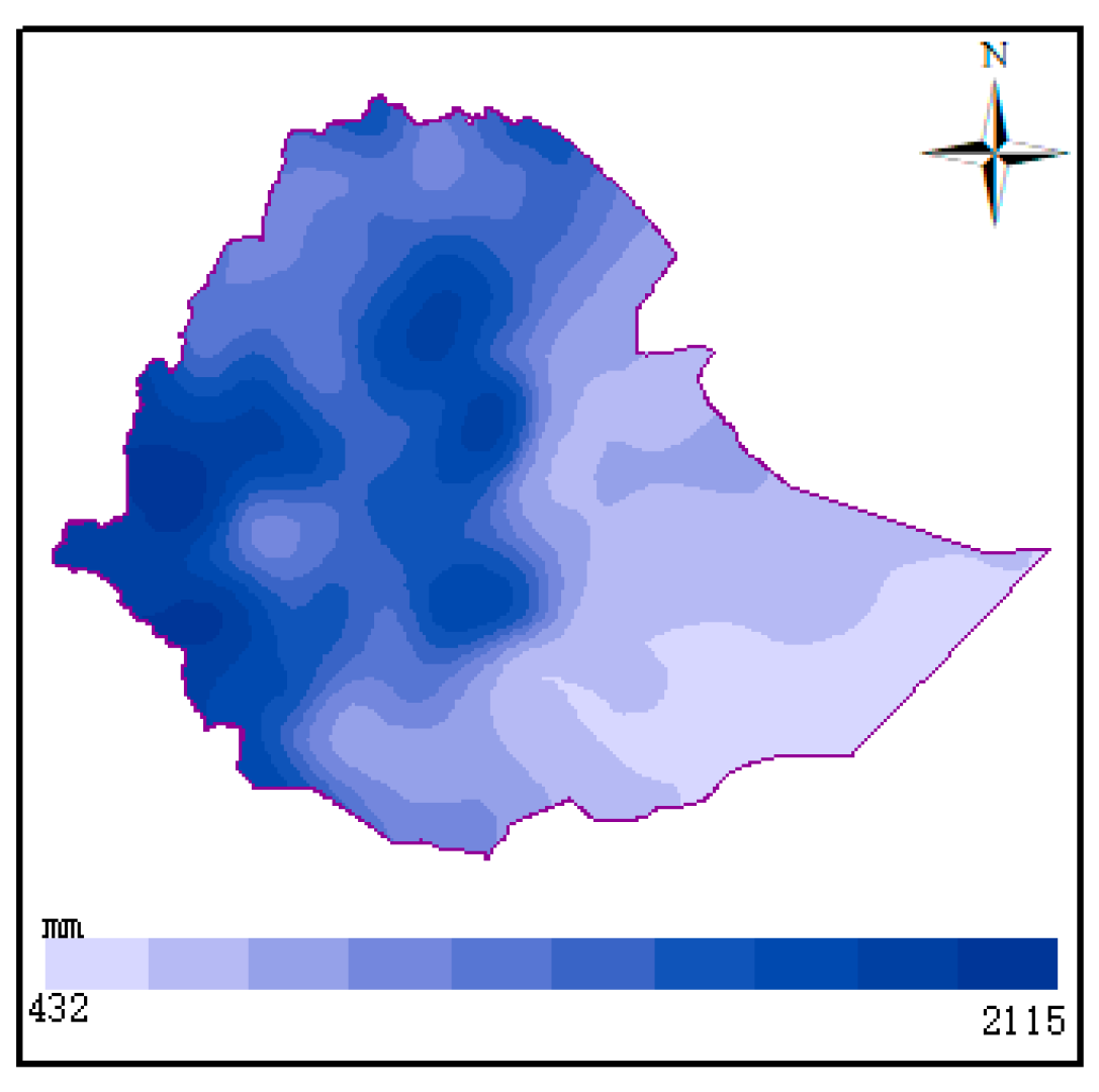
The high-resolution spatial distribution map of the mean annual precipitation in Ethiopia from 1990 to 2020 is shown in Figure 4. The East African Rift Valley divides Ethiopia into an eastern flat lowland region and a western highland region. By comparing the mean annual precipitation distribution (Figure 4) and topographic features (Figure 2), an obvious difference in annual precipitation between the eastern and western regions was found. Ethiopia’s precipitation was significantly affected by altitude: it went from an arid climate in the eastern flat lowland region to a humid climate in the western highland region. The annual precipitation in Ethiopia was mainly concentrated in the western highland regions, and it increased with altitude. The eastern lowland region had a flat terrain and significantly less precipitation. Figure 5 shows high-resolution maps of the monthly average precipitation generated by our hybrid of MLPs. Less precipitation occurred from December to February. From May to October, affected by the humid southeast monsoon, the precipitation gradually increased; in particular, the precipitation reached the maximum during June to August.

4.2.2. Air Temperature

We used the hybrid of MLPs to downscale the sparse air temperature observations and generated an air temperature map with a resolution of 0.1° × 0.1°. The two statistical indicators in

Table 3. Accuracy of high-resolution air temperature maps generated using three models.

Models	MAPE (%)		R2
	Range	Mean	Range	Mean
Multi-linear regression	1.48–6.94	4.09	0.65–0.88	0.76
Pure MLP	2.13–6.33	3.80	0.75–0.91	0.82
Hybrid of MLPs	0.98–2.77	1.96	0.84–0.93	0.90

showed the downscaling performance of our hybrid of MLPs, a pure MLP and multi-linear regression. Our hybrid of MLPs showed significantly better downscaling performance than multi-linear regression. The MAPE value attained when using the hybrid of MLPs was 0.5~4.17% lower than that found when using the multi-linear regression, the $R^2$ values attained when using hybrid of MLPs was 0.05–0.19 higher than that found when using multi-linear regression. The hybrid of MLPs was also better than the pure MLP: the R² value attained when using the hybrid of MLPs was increased by 0.08 and the MAPE value was decreased by 2.13.

The high-resolution map of Ethiopia’s mean annual air temperature generated using the hybrid of MLPs is shown in Figure 6. During 1990–2020, the mean annual air temperature in Ethiopia was about 16–28 °C. By comparing the mean annual air temperature distribution (Figure 6) and topographic features (Figure 2), the annual air temperature in Ethiopia significantly decreased with the increase in altitude: it went from a hot climate in the eastern terrain to a cool climate in the western plateau. Since the central region is the Ethiopian plateau with an average altitude of nearly 3000 m, the air temperature for this region was the lowest in Ethiopia. The high air temperature was mainly concentrated in the northeast and southeast, and the highest annual air temperature reached 28 °C.

The high-resolution monthly air temperature maps generated using the hybrid of MLPs are shown in Figure 7. The air temperature in Ethiopia gradually increased from March to August, with the highest air temperature of 31 °C. The coldest months in Ethiopia were November and December, where the lowest air temperature reached 13 °C. From the monthly air temperature high-resolution map, it was found that the climate in Ethiopia was characterized by a high air temperature in summer and a low temperature in winter. The air temperature decreased with altitude. In most months, the air temperature in the central region was lower than that in other regions.

5. Conclusions

Many developing countries are extremely vulnerable to climate change due to their rain-fed agriculture, weak industry basis and backward infrastructure. At the same time, meteorological stations in these developing countries are always sparse and irregularly distributed; these limited climate observations are insufficient to meet the needs of mitigating climate risks and improving resilience and adoption measures. Mainstream geostatistical downscaling techniques use spatial interpolation or multi-linear regression to produce high-resolution climate maps. Since global climate evolution is a nonlinear process governed by complex physical principles, these linear downscaling techniques cannot achieve the desired accuracy. The latest statistical learning techniques can extract nonlinear relations, but they cannot use different-resolution observation data as model inputs. In this study, we developed a hybrid of MLPs to solve these issues.

Our hybrid of MLPs not only fully coupled different-resolution observation data but also identified the complex nonlinear relationships without considering physical principles in advance. Compared with existing geostatistical algorithms, our hybrid of MLPs is the first geostatistical algorithm to utilize a strong link between observed climate variables to generate high-resolution climate maps. Our algorithm does not need to use a huge amount of GCM outputs like the statistical downscaling model (SDSM) does and has a simple network structure, and thus, its computation cost is very low. As a demonstration experiment, we generated high-resolution precipitation and air temperature maps using sparse observation data from 21 meteorological stations in Ethiopia. The accuracy of the high-resolution climate maps generated using our hybrid of MLPs clearly outperformed those created using a multi-linear regression model or a pure MLP. If we can obtain observations of more climate variables (e.g., humidity, wind and atmospheric pressure) at these Ethiopian meteorological stations, higher accuracy high-resolution climate maps can be achieved. Although we only demonstrated the generation of high-resolution Ethiopian climate maps, our hybrid of MLPs can generate high-resolution climate maps from sparse observation data in any developing country.