Mathematical Circuit Root Simplification Using an Ensemble Heuristic–Metaheuristic Algorithm

Abstract

Symbolic pole/zero analysis is a crucial step in designing an analog operational amplifier. Generally, a simplified symbolic analysis of analog circuits suffers from NP-hardness, i.e., an exponential growth of the number of symbolic terms of the transfer function with the circuit size. This study presents a mathematical model combined with a heuristic–metaheuristic solution method for symbolic pole/zero simplification in operational transconductance amplifiers. First, the circuit is symbolically solved and an improved root splitting method is applied to extract symbolic poles/zeroes from the exact expanded transfer function. Then, a hybrid algorithm based on heuristic information and a metaheuristic technique using simulated annealing is used for the simplification of the derived symbolic roots. The developed method is tested on three operational transconductance amplifiers. The obtained results show the effectiveness of the proposed method in achieving accurate simplified symbolic pole/zero expressions with the least complexity.

1. Introduction

Symbolic analysis is a method of analyzing analog circuits in which the circuit equations are expressed in terms of symbolic variables. This technique is useful for designing and analyzing complex analog circuits (especially those with nonlinear components) as it provides engineers with a deep insight into the relations between the circuit variables rather than simply relying on numerical methods. Therefore, this method can help circuit designers to quickly evaluate different design alternatives by allowing them to manipulate circuit equations algebraically, enabling the study of the effects of different component values on the circuit performance. One of the major applications of symbolic analysis is to determine the location and characteristics of circuits’ poles and zeroes, which is needed to analyze the stability and frequency response of the circuit [1].

Recently, multi-stage operational transconductance amplifiers (OTAs) have become widely applied in modern microelectronics, as OTAs can provide a large output swing and high gain with very low overdrive voltage [2]. However, as each stage has its own poles and zeroes, the bandwidth may be reduced. In addition to the poles and zeroes of each additional stage, the compensated capacitors may add some extra poles and zeroes [3]. One of the main challenges in the design of multi-stage OTAs is to devise a frequency compensation procedure capable of providing wide bandwidth and high gain with appropriate stability margins [4]. In this regard, a simplified extraction of symbolic poles and zeroes can give better analytical expressions and assist designers in making a straight decision when designing an OTA and a frequency compensation circuit [5].

Generally, an exact symbolic analysis of OTAs is error-prone and time-consuming if performed by hand, even for circuits with a small number of components [6]. In this regard, a computer-aided automatic symbolic analysis can be helpful by solving the circuit equations with mathematical solvers such as Cramer’s rule [7]. It can be performed by exploiting symbolic analysis solvers using software tools such as MATLAB, GNU Octave, and MAPLE [8]. The main drawbacks of a symbolic analysis are that the derived symbolic equations are very complex and cannot effectively guide the circuit designer [9]. Although various symbolic simplification techniques have been introduced, simplified expressions are not provided in a factorization form. Thus, it is difficult to evaluate the effects of roots on the behavior of the circuit.

Although the existing symbolic pole/zero analysis methods incorporate some types of approximations during the calculation of the transfer function, they suffer from some drawbacks which limit their effectiveness for use in real-world OTAs. First, these methods are inefficient in the case of overall generated error rates in terms of magnitude, phase, poles and zeroes [10]. Second, the correlation between eliminated terms in different polynomials is not effectively considered in polynomial-oriented methods. Third, pole/zero displacements due to approximations are not under control [7]. Fourth, those closely spaced pole/zero pairs may disappear due to a magnitude-/phase-oriented approximation, which can generate high error rates at points other than the nominal ones [8].

Over the past years, metaheuristics have also been presented for use in the parameter selection and symbolic simplification in electrical circuits. Shokouhifar and Jalali [10] presented a combined algorithm based on the genetic algorithm (GA) and simulated annealing (SA) as a metaheuristic-based optimization technique for symbolic term selection in the symbolic voltage gain of analog circuits containing transistors. Akbari et al. [3] proposed a symbolic analysis for the design of analog integrated circuits using an ant colony optimization (ACO) algorithm which takes noise optimization into account. Another technique, outlined in [11], involved performing GA, SA, and particle swarm optimization (PSO) to simplify the symbolic expressions for the common-mode rejection ratio (CMRR) and power supply rejection ratio (PSRR) of the analog amplifier. Sathasivam et al. [12] presented a combined metaheuristic algorithm based on GA and tabu search (TS) with restricted neural symbolic integration for solving the maximum k-satisfiability problem. Ali et al. [13] proposed a new hybrid metaheuristic algorithm based on the marine predator algorithm and sine cosine algorithm for selecting the best parameters for hybrid active power filters.

Although various metaheuristics have been presented for circuit simplification, they mostly present symbolic expressions in expanded forms. The existing symbolic root simplification techniques typically use simple criteria which are separately applied to each polynomial of the exact symbolic roots. Thus, these techniques do not guarantee a good match of the simplified root expressions compared to the exact ones. Although the maximum error of each simplified polynomial is limited, the displacement of poles and zeroes is not under control [7]. Therefore, despite the simplicity of the traditional methods, they may generate large errors in the simplified root expressions.

In this study, a simplified symbolic pole/zero extraction technique is presented based on an extension of the root splitting technique [14] and SA [15]. In this regard, we first introduce an enhanced root splitting (named ERS) for the symbolic pole/zero extraction from the exact transfer function. In this method, pole/zero displacements cannot exceed a pre-specified threshold. Then, we apply a metaheuristic-driven simplification method based on SA (named PZSA) to simplify the derived pole/zero expressions. Our main motivation is to mathematically formulate the pole/zero simplification problem in analog circuits as a multi-objective constrained optimization problem. The established problem can be solved by the use of optimization algorithms such as heuristics, single-solution metaheuristics, or population-based evolutionary and swarm intelligence algorithms. Thus, this paper applies a combined heuristic–metaheuristic algorithm based on the heuristic information available in the circuit model and SA to solve the symbolic root simplification problem. The key contributions outlined in this study can be characterized as follows:

• Introducing a combined mathematical modeling and optimization technique for the extraction and simplification of symbolic poles and zeros in OTAs.
• Proposing an enhanced root splitting technique, named ERS, to accurately extract the exact pole/zero expressions.
• Applying a combined heuristic–metaheuristic optimization algorithm to solve the proposed symbolic root simplification problem, utilizing the heuristic knowledge available in the circuit model and SA.
• Programming the proposed method in a MATLAB m-file, wherein simplified root equations are automatically generated from the circuit netlist.
• Successfully driving symbolic pole/zero expressions for three OTAs.

The rest of this study is organized as follows: In Section 2, the existing literature for a symbolic simplification and symbolic pole/zero extraction is reviewed. In Section 3, the proposed methodology is presented with details, and then the developed method in MATLAB is evaluated in Section 4. Finally, in Section 5, some concluding remarks are made and future directions are addressed.

2. Literature Review

Over recent years, along with the increasing advancement and development in analog circuit design, various symbolic simplification techniques and symbolic pole/zero extraction methods have been proposed. According to the existing literature, these methods can be described in the following manners outlined below.

2.1. Symbolic Simplification Techniques

The symbolic analysis of OTAs suffers from NP-hardness [7]. For instance, the μA741 amplifier has approximately 10³⁴ terms within its voltage transfer function [16]. Therefore, symbolic analysis tools must rely on simplification techniques to tackle the complexity and hardness of real-world circuits. Based on the steps taken in the simplification process, simplification algorithms can be categorized into SAG (simplification-after-generation), SDG (simplification-during-generation), and SBG (simplification-before-generation) [17]. It is worth noting that the proposed PZSA algorithm in this study is an SAG technique. An SAG is performed once the symbolic circuit analysis is done and, as a result, the exact symbolic expressions have been obtained. Therefore, simplified functions can be constructed from some terms of the exact expressions. In the following section, we discuss the details of the SAG technique used in the proposed method.

The small-signal transfer function of a linear or linearized circuit can be represented as a function of the frequency $s$ and the circuit parameters $\mathbf{x}$, according to Equation (1) [8], where each polynomial ${\acute{f}}_i\left(\mathbf{x}\right)$ or $f_i\left(\mathbf{x}\right)$ is a sum-of-product (SOP) of $\mathbf{x}$. This is expressed as $h_k\left(\mathbf{x}\right)=h_{k1}\left(\mathbf{x}\right)+h_{k2}\left(\mathbf{x}\right)+\dots +h_{kT}\left(\mathbf{x}\right)$, where $h_k\left(\mathbf{x}\right)$ is the $k$-th polynomial within the circuit transfer function $H\left(s,\mathbf{x}\right)$, comprising $T$ terms.

$$H(s,\mathbf{x})=\frac{N(s,\mathbf{x})}{D(s,\mathbf{x})}=\frac{{f^{\prime }}_0\left(\mathbf{x}\right)+{f^{\prime }}_1\left(\mathbf{x}\right)s+{f^{\prime }}_2\left(\mathbf{x}\right)s^2+\dots +{f^{\prime }}_{n^{\prime }}\left(\mathbf{x}\right)s^{n^{\prime }}}{f_0\left(\mathbf{x}\right)+f_1\left(\mathbf{x}\right)s+f_2\left(\mathbf{x}\right)s^2+\dots +f_n\left(\mathbf{x}\right)s^n}$$

(1)

The simplification method in [18] finds the largest term in terms of the magnitude, $h_{km}\left(\mathbf{x}\right)$, for the polynomial $h_k\left(\mathbf{x}\right)$. Then, all other terms within the polynomial $h_k\left(\mathbf{x}\right)$ are considered one by one. The condition for which the term $h_{kl}\left(\mathbf{x}\right)$ can be discarded from the polynomial $h_k\left(\mathbf{x}\right)$ is $\left|h_{kl}\left(\mathbf{x}\right)\right|\le \epsilon \times \left|h_{km}\left(\mathbf{x}\right)\right|$. Here, $\epsilon$ (0 < $\epsilon$ < 1) is a user-specified threshold to limit the maximum error. The main drawback of this method is that the error may be accumulated. To overcome this drawback, the reported criterion in [19] sorts the terms within $h_k\left(\mathbf{x}\right)$ based on their magnitude obtained in the nominal point. Afterwards, $P$ terms with the least accumulated magnitude are discarded from the polynomial if the error is below $\epsilon$. The condition on the $P$ terms for which they could be discarded can be expressed as Equation (2):

$$\left|{\displaystyle \sum _{l=1}^P}{h}_{kl}\left(\mathbf{x}\right)\right|<\epsilon \times \left|{\displaystyle \sum _{l=1}^T}{h}_{kl}\left(\mathbf{x}\right)\right|$$

(2)

Although this method achieves more accurate expressions at the nominal point, it may cause significant errors for other values of the parameters. To avoid the elimination of the mutually canceling terms, the method in [20] presented an enhanced condition for which the $P$ terms with the lowest magnitude can be discarded if:

$${\displaystyle \sum _{l=1}^P}\left|h_{kl}\left(\mathbf{x}\right)\right|<\epsilon \times {\displaystyle \sum _{l=1}^T}\left|h_{kl}\left(\mathbf{x}\right)\right|$$

(3)

In the above-mentioned techniques, the maximum error is limited for each polynomial. However, the obtained error in the poles and zeroes is not under consideration. If the same error (${\epsilon }_M$) occurs in all polynomials, no pole and/or zero displacement can be observed [21]. To overcome this drawback, an adaptive $\epsilon$ can be used, in which the term elimination process is performed step by step while displacements in poles and zeroes are monitored at every step. Thus, the term pruning procedure can be finished if the obtained displacements are beyond a pre-determined threshold [19].

Recently, various swarm and evolutionary metaheuristic algorithms in [7,10,22,23,24,25,26] have been applied for the simplified symbolic analysis of OTAs. In these techniques, different criteria (such as the magnitude error, phase error, and pole/zero displacements) have been used to evaluate feasible solutions generated by the metaheuristic algorithm. Although these methods achieve a low mean error rate, the worst cases of the displacements in the poles and zeroes are not accurately under consideration. The common drawback of the existing techniques is that the simplified function is achieved in either expanded or nested form. In other words, the transfer function is not derived in a factorization form, which makes it difficult to evaluate the contribution of roots.

2.2. Symbolic Pole/Zero Extraction Techniques

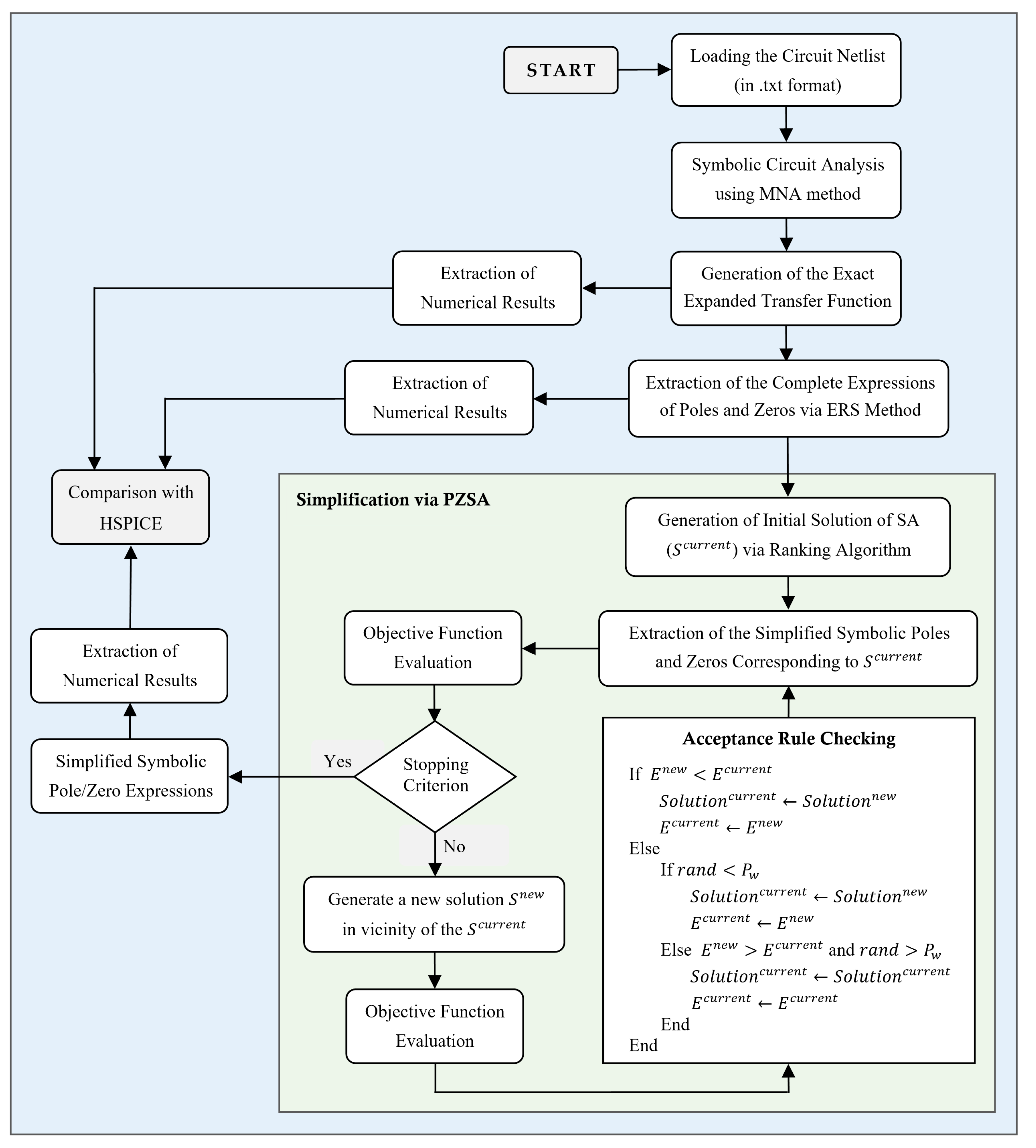
The symbolic pole/zero analysis also suffers from NP-hardness as some operations have to be performed between the polynomials. Generally, a direct calculation of the roots from the expanded transfer functions yields very complex results in the form of polynomials with degrees larger than two [7]. Since the numerator and denominator of a transfer function in practical OTAs generally have degrees much larger than 2, it is rarely possible to mathematically find the exact symbolic pole/zero expressions [27].

In the following section, the existing pole/zero extraction methods are discussed, including root spitting, time-constant analysis, and eigenvalue analysis. Root splitting [14] is one of the well-known root extraction techniques. It extracts poles, assuming them to be reciprocally dominant. By factorization, the denominator of the exact function in Equation (1) can be re-written as a function of the poles $p_i$ as follows:

$$D(s,\mathbf{x})=f_0\cdot \left(1-\frac{s}{p_1}\right)\cdot \left(1-\frac{s}{p_2}\right)\cdots \left(1-\frac{s}{p_n}\right)$$

(4)

It follows from Equation (1) that

$$f_1=f_0\cdot {\displaystyle \sum _{i=1}^n}\left(-\frac{1}{p_i}\right)$$

(5)

Therefore, assuming $p_1$ is the dominant pole within the denominator, the first pole can be approximately expressed as:

$$p_1\approx -\frac{f_0}{f_1}$$

(6)

Consequently, with a similar approach, considering $p_i$ to dominate the other poles, $p_i$ can be given by the negative quotient of the two consecutive coefficients $f_{i-1}$ and $f_i$ [8]. Similar argumentations can be performed to calculate simplified zeroes in the numerator of the transfer function. The root splitting method is not appropriate for manual pole/zero calculations (hand-and-paper analysis), as some estimations and simplifications should be developed to allow the circuit designer to extract approximate the dominant poles and zeroes manually. The most popular approach in such techniques is the time-constant method [27,28,29,30], which is expressed in Equation (7), where ${\tau }_k$ can be achieved by multiplying the resistance $R_k$ by the capacitance $C_k$.

$$p_1\approx -{\left(\sum _k{\tau }_k\right)}^{-1}$$

(7)

This technique is error-prone, as there is no information about the accuracy of the obtained symbolic results. Moreover, zeroes and higher-order poles cannot be determined by this approach at all. A more general approach in this context was reported in [29], one which also has the ability to extract the higher-order poles. This method is based on the use of open-circuits and short-circuits analysis to calculate the time constants of the circuit.

There are also some pole/zero extraction methods, which operate on the basis of the solution derived from the eigenvalue problem. A positive feature of these methods is that the simplification is no longer driven by the magnitude and the phase errors but by the pole/zero position, allowing improved error control. For example, a modified signal flow graph (MSFG) was recently developed to represent the equivalences between the system and SPICE outcomes of static nonlinear OTAs [31]. In this method, the circuit is firstly converted into an MSFG. Then, the graph is simplified in particular polynomials by minimizing the MSFGs. In [32], the implementation of some simplification procedures during the eigenvalue computation via a symbolic LR algorithm was addressed, in which the LR method is applied to compute the reduced matrix corresponding to the eigenvalue cluster. This technique is followed in [33] by the use of an algorithm to reduce the circuit matrix into a row echelon format. After determining the symbolic state matrix, the approximated poles and zeroes are achieved using the LR algorithm.

The main drawback of the existing symbolic pole/zero analysis methods is that the simplified expressions of poles and zeroes are not so compact that no SAG is applied to the final expressions. Thus, in this study, we utilize a combined heuristic–metaheuristic SAG algorithm to ensure the obtention of simplified symbolic pole/zero expressions with the least achievable complexity.

3. Proposed Method

The overall flowchart of the proposed symbolic pole/zero analysis can be seen in Figure 1. The list of indices, sets, parameters, and decision variables used in the following equations of this section are provided in

Table 1. Notations.

Sets/Parameters	Definition
$i$	Index of poles, $i=\mathrm{1,2},\dots ,n$
$j$	Index of zeroes, $j=\mathrm{1,2},\dots ,\acute{n}$
$n$	Degree of the denominator within the exact expanded TF
$\acute{n}$	Degree of the numerator within the exact expanded TF
$k$	Index of the symbolic terms, $k=\mathrm{1,2},\dots ,L$
$L$	Number of symbolic terms within all pole/zero expressions
$[f_{min},f_{max}]$	Defined frequency bound range for the pole/zero extraction
$S_k$	A binary parameter: 1 if the $k$-th term is presented; 0 otherwise
$E_n$	Percentage of the selected symbolic terms
$PoleSet$	Set of poles in the frequency range of $[f_{min},f_{max}]$
ZeroSet	Set of zeroes in the frequency range of $[f_{min},f_{max}]$
$p_{E,i}$	$i$-th pole within the exact expanded TF
$p_{ERS,i}$	$i$-th extracted pole via ERS
$p_{SA,i}$	$i$-th simplified pole via SA
$E_p$	Mean pole displacements
$z_{E,j}$	$j$-the zero of the exact expanded TF
$z_{ERS,j}$	$j$-th extracted zero via ERS
$z_{SA,j}$	$j$-th simplified zero via SA
$E_z$	Mean zero displacements
$T_{ERS}$	Maximum allowable pole/zero extraction error via ERS
$T_{SA}$	Maximum allowable pole/zero simplification error via SA

. To sum up, the main steps of the proposed methodology can be summarized as follows:

• The input circuit netlist is loaded as a text file (in .txt format).
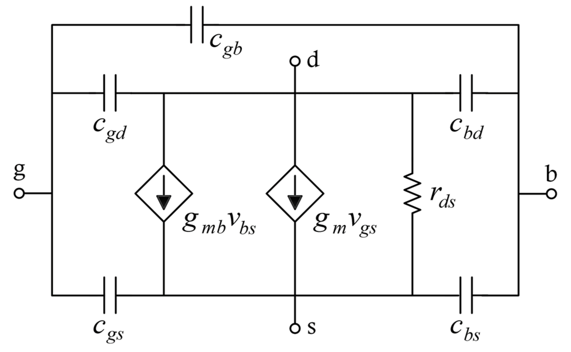
• All transistors are replaced via proper small-signal modeling.
• The symbolic circuit is solved via a modified nodal analysis (MNA).
• The exact transfer function (TF) is achieved in the expanded symbolic form.
• The exact expressions of poles and zeroes are derived using ERS.
• The numerical results of the exact symbolic pole/zero expressions are stored.
• A heuristic algorithm is performed to generate a near-optimal solution, utilizing the circuit-based knowledge available in the exact poles and zeroes.
• SA is performed to improve further the quality of the heuristic solution in order to generate the final simplified symbolic pole/zero expressions.
• The numerical results of the obtained simplified symbolic pole/zero expressions are calculated.
• The numerical results of the exact and simplified poles/zeroes are compared against HSPICE and other simplification algorithms.

3.1. Symbolic Pole/Zero Extraction via ERS

After the netlist pre-processing, the circuit is solved using MNA [1], and consequently, the exact symbolic TF is achieved in expanded form. Then, the obtained exact pole/zero expressions are approximately calculated using the proposed ERS method, which is an enhanced version of the traditional root splitting algorithm. Generally, an expanded TF could be converted into the factorized form according to Equation (8), where $Z(s,\mathbf{x})$ is a function of $\acute{n}$ (real or complex conjugate) zeroes $z_1$, $z_2$, …, $z_{\acute{n}}$, and $P(s,\mathbf{x})$ is a function of $n$ (real or complex conjugate) poles $p_1$, $p_2$, …, $p_n$.

$$(s,\mathbf{x})\approx \frac{{f^{\prime }}_0\cdot Z(s,\mathbf{x})}{f_0\cdot P(s,\mathbf{x})}$$

(8)

In the ERS algorithm, only poles and zeroes located in the interval [$f_{min},f_{max}]$ are extracted, where $f_{min}$ and $f_{max}$ are the minimum and maximum user-specified frequencies for the pole/zero extraction, respectively. If the user does not specify the frequency range, it is considered as the default range of [$\mathrm{0,10}{f}_T]$, where $f_T$ is the unity gain frequency of the exact expression in the nominal point. In the following section, the pole extraction procedure for $P(s,\mathbf{x})$ is described. By comparing Equations (1) and (8), $P(s,\mathbf{x})$ can be calculated as:

$$P(s,\mathbf{x})=\frac{D(s,\mathbf{x})}{f_0}=1+\left(\frac{f_1}{f_0}\right)s+\left(\frac{f_2}{f_0}\right)s^2+\left(\frac{f_3}{f_0}\right)s^3+\cdots +\left(\frac{f_n}{f_0}\right)s^n$$

(9)

Assuming $p_1$ to be dominant and all other poles (typically occurred in OTAs) to be located at much higher frequencies, i.e., $‖p_1‖<<‖p_2‖,‖p_3‖,\dots ,‖p_n‖$, the first pole can be split, and thus, $P(s,\mathbf{x})$ can be approximately written as:

$$\begin{array}{l}P(s,\mathbf{x})=\left(1-\frac{s}{p_1}\right)\cdot \left(1+g_{1}s+g_2{s}^2+\cdots +g_{n-1}{s}^{n-1}\right)\\ \hspace{1em}\hspace{1em}\hspace{1em}=1+\left(-\frac{1}{p_1}+g_1\right)s+\left(-\frac{g_1}{p_1}+g_2\right)s^2+\left(-\frac{g_2}{p_1}+g_3\right)s^3+\cdots +\left(-\frac{g_{n-2}}{p_1}+g_{n-1}\right)s^{n-1}+\left(-\frac{g_{n-1}}{p_1}\right)s^n\end{array}$$

(10)

By equating the $s$ coefficients of $P(s,\mathbf{x})$ in Equation (10) to those in Equation (9), the dominant real pole $p_1$ can be approximated given as:

$$p_1\approx -\frac{f_0}{f_1}$$

(11)

Consequently, by assuming the condition in Equation (12), we can simplify the rightmost expression of Equation (10) as Equation (13). By equating the $s$ coefficients of Equation (13) to the same $s$ coefficients in Equation (9), the parameters $g_i$ can be calculated as Equation (14).

$$\left|\frac{1}{p_1}\right|>>\left|g_1\right|, \left|\frac{g_{i-1}}{p_1}\right|>>\left|g_i\right|\hspace{1em}\hspace{1em}\hspace{1em}\forall i\in \{\mathrm{2,3},\dots ,n-1\}$$

(12)

$$P(s,\mathbf{x})\approx 1+\left(-\frac{1}{p_1}\right)s+\left(-\frac{g_1}{p_1}\right)s^2+\left(-\frac{g_2}{p_1}\right)s^3+\cdots +\left(-\frac{g_{n-1}}{p_1}\right)s^n$$

(13)

$$g_i=\frac{f_{i+1}}{f_1}\hspace{1em}\hspace{1em}\forall i\in \{\mathrm{1,2},\dots ,n-1\}$$

(14)

and thus, the leftmost expression in Equation (10) can be expressed as:

$$P(s,\mathbf{x})\approx \left(1+\frac{f_1}{f_0}s\right)\cdot \left(1+\frac{f_2}{f_1}s+\frac{f_3}{f_1}{s}^2+\cdots +\frac{f_n}{f_1}{s}^{n-1}\right)$$

(15)

The circumstances of $s$ coefficients in the original denominator $D(s,\mathbf{x})$, for which Equation (15) is valid, are:

$$\left|\frac{f_1}{f_0}\right|>>\left|\frac{f_i}{f_{i-1}}\right|\hspace{1em}\hspace{1em}\forall i\in \{\mathrm{2,3},\dots ,n\}$$

(16)

Equation (15) shows that $P(s,\mathbf{x})$ can be simplified into a product of a first-order polynomial (i.e., first dominant pole) and a high-order polynomial corresponding to other high-frequency poles. In a more general case, assuming the first $m$ poles ($1<m<n$) to be successively dominant in pairs (i.e., $p_1$ dominates $p_2$, $p_2$ dominates $p_3$, and so on, $p_{m-1}$ dominates $p_m$), $P(s,\mathbf{x})$ can be approximated as follows:

$$\begin{array}{l}P(s,\mathbf{x})=\left(1-\frac{s}{p_1}\right)\cdot \left(1-\frac{s}{p_2}\right)\cdots \left(1-\frac{s}{p_m}\right)\cdot \left(1+g_{1}s+g_2{s}^2+\cdots +g_{n-m}{s}^{n-m}\right)\\ \hspace{1em}\hspace{1em}\hspace{1em}=1+\left(-{\displaystyle {\displaystyle \sum _{i=1}^m}}\frac{1}{p_i}+g_1\right)s+\left({\displaystyle \sum _{i=1}^{m-1}}{\displaystyle {\displaystyle \sum _{j=i+1}^m}}\frac{1}{p_i{p}_j}-g_1{\displaystyle \sum _{i=1}^m}\frac{1}{p_i}+g_2\right)s^2\\ \hspace{1em}\hspace{1em}\hspace{1em}\hspace{1em}+\left(-{\displaystyle \sum _{i=1}^{m-2}}{\displaystyle {\displaystyle \sum _{j=i+1}^{m-1}}}{\displaystyle \sum _{k=j+1}^m}\frac{1}{p_i{p}_j{p}_k}+g_1{\displaystyle \sum _{i=1}^{m-1}}{\displaystyle {\displaystyle \sum _{j=i+1}^m}}\frac{1}{p_i{p}_j}-g_2{\displaystyle \sum _{i=1}^m}\frac{1}{p_i}+g_3\right)s^3+\cdots \\ \hspace{1em}\hspace{1em}\hspace{1em}\hspace{1em}+\left((-1{)}^m{g}_{n-m-1}{\displaystyle \prod _{i=1}^m}\frac{1}{p_i}+(-1{)}^{m-1}{g}_{n-m}{\displaystyle \sum _{i_1=1}^2}{\displaystyle \sum _{i_2=i_1+1}^3}\cdots {\displaystyle \sum _{i_{m-1}=i_{m-2}+1}^m}\frac{1}{p_{i_1}{p}_{i_2}{p}_{i_{m-1}}}\right)s^{n-1}+\left((-1{)}^m{g}_{n-m}{\displaystyle \prod _{i=1}^m}\frac{1}{p_i}\right)s^n\end{array}$$

(17)

By similar approximations as performed in the previous case, $P(s,\mathbf{x})$ can be simplified according to:

$$\begin{array}{l}P(s,\mathbf{x})\approx 1+\left(-\frac{1}{p_1}\right)s+\left(\frac{1}{p_1{p}_2}\right)s^2+\left(-\frac{1}{p_1{p}_2{p}_3}\right)s^3+\cdots +\left((-1{)}^m{\displaystyle \prod _{i=1}^m}\frac{1}{p_i}\right)s^m+\cdots \\ \hspace{1em}\hspace{1em}\hspace{1em}+\left((-1{)}^m{g}_1{\displaystyle \prod _{i=1}^m}\frac{1}{p_i}\right)s^{m+1}+\cdots +\left((-1{)}^m{g}_{n-m-1}{\displaystyle \prod _{i=1}^m}\frac{1}{p_i}\right)s^{n-1}+\left((-1{)}^m{g}_{n-m}{\displaystyle \prod _{i=1}^m}\frac{1}{p_i}\right)s^n\end{array}$$

(18)

By equating the $s$ coefficients of Equations (18) and (9), the $m$ first poles are derived as Equation (19). Additionally, the parameters $g_i$ can be expressed as Equation (20). Thus, $P(s,\mathbf{x})$ can be simplified into the multiplication of $m$+1 polynomials: $m$ first-order polynomials (representing the $m$ first poles) and a high-order polynomial, as Equation (21). The conditions on $s$ coefficients of $D(s,\mathbf{x})$, for which Equation (21) is valid, can be expressed as Equations (22) and (23).

$$p_i=-\frac{f_{i-1}}{f_i}\hspace{1em}\hspace{1em}\forall i\in \{\mathrm{1,2},\dots ,m\}$$

(19)

$$g_i=\frac{f_{m+i}}{f_m}\hspace{1em}\hspace{1em}\forall i\in \{\mathrm{1,2},\dots ,n-m\}$$

(20)

$$P(s,\mathbf{x})=\left(1+\frac{f_1}{f_0}s\right)\cdot \left(1+\frac{f_2}{f_1}s\right)\cdots \left(1+\frac{f_m}{f_{m-1}}s\right)\cdot \left(1+\frac{f_{m+1}}{f_m}s+\frac{f_{m+2}}{f_m}{s}^2+\cdots +\frac{f_n}{f_m}{s}^{n-m}\right)$$

(21)

$$\left|\frac{f_i}{f_{i-1}}\right|>>\left|\frac{f_{i+1}}{f_i}\right|\hspace{1em}\hspace{1em}\forall i\in \{\mathrm{1,2},\dots ,m-1\}$$

(22)

$$\left|\frac{f_i}{f_{i-1}}\right|>>\left|\frac{f_j}{f_{j-1}}\right|\hspace{1em}\hspace{1em}\forall i\in \{\mathrm{1,2},\dots ,m\},j\in \{m+1,m+2,\dots ,n\}$$

(23)

In the general case, let us extend the above formulations to the case that all the $n$ poles are dominant reciprocally, in which $P(s,\mathbf{x})$ can be approximated as follows:

$$\begin{array}{l}P(s,\mathbf{x})=\left(1-\frac{s}{p_1}\right)\cdot \left(1-\frac{s}{p_2}\right)\cdot \left(1-\frac{s}{p_3}\right)\cdots \left(1-\frac{s}{p_n}\right)\\ \hspace{1em}\hspace{1em}=1+\left(-{\displaystyle \sum _{i=1}^n}\frac{1}{p_i}\right)s+\left({\displaystyle \sum _{i=1}^{n-1}}{\displaystyle \sum _{j=i+1}^n}\frac{1}{p_i{p}_j}\right)s^2+\left(-{\displaystyle \sum _{i=1}^{n-2}}{\displaystyle \sum _{j=i+1}^{n-1}}{\displaystyle \sum _{k=j+1}^n}\frac{1}{p_i{p}_j{p}_k}\right)s^3\\ \hspace{1em}\hspace{1em}+\cdots +\left((-1{)}^{n-1}{\displaystyle \sum _{i_1=1}^2}{\displaystyle \sum _{i_2=i_1+1}^3}\cdots {\displaystyle \sum _{i_{n-1}=i_{n-2}+1}^n}\frac{1}{p_{i_1}{p}_{i_2}{p}_{i_{n-1}}}\right)s^{n-1}+\left((-1{)}^n{\displaystyle \prod _{i=1}^n}\frac{1}{p_i}\right)s^n\end{array}$$

(24)

Under the assumption that all poles are dominant in pairs (i.e., $p_1$ dominates $p_2$, $p_2$ dominates $p_3$, and so on), the following conditions are satisfied:

$$\left|\frac{f_i}{f_{i-1}}\right|>>\left|\frac{f_{i+1}}{f_i}\right|\hspace{1em}\hspace{1em}\forall i\in \{\mathrm{1,2},3,\dots ,n-1\}$$

(25)

Therefore, the rightmost expression in Equation (24) can be approximated as Equation (26). By equating $s$ coefficients of Equation (26) and Equation (9), $P(s,\mathbf{x})$ can be approximately expressed as Equation (27), where each pole $p_i$ can be calculated according to Equation (28).

$$P(s,\mathbf{x})\approx 1+\left(-\frac{1}{p_1}\right)s+\left(\frac{1}{p_1{p}_2}\right)s^2+\cdots +\left((-1{)}^{n-1}{\displaystyle \prod _{i=1}^{n-1}}\frac{1}{p_i}\right)s^{n-1}+\left((-1{)}^n{\displaystyle \prod _{i=1}^n}\frac{1}{p_i}\right)s^n$$

(26)

$$P(s,\mathbf{x})\approx \left(1+\frac{f_1}{f_0}s\right)\cdot \left(1+\frac{f_2}{f_1}s\right)\cdot \left(1+\frac{f_3}{f_2}s\right)\cdots \left(1+\frac{f_n}{f_{n-1}}s\right)$$

(27)

$$p_i=-\frac{f_{i-1}}{f_i}\hspace{1em}\hspace{1em}\forall i\in \{\mathrm{1,2},\dots ,n\}$$

(28)

The interesting point is that all poles are derived from $s$ coefficients of the denominator of the transfer function. The above formulations operate under the assumption that all poles are real. In other words, the approach fails for closely spaced or complex conjugate poles. Therefore, the method should be extended to cases where two consecutive poles are located in a cluster. Assuming that $p_i$ and $p_{i+1}$ constitute a pair of poles (real or conjugate), they remain split off in the expression $P(s,\mathbf{x})$ and can be expressed via a second-order polynomial $(1+as+b{s}^2)$, where $a$ and $b$ can be calculated as follows:

$$a=\frac{f_i}{f_{i-1}}+\frac{f_{i+1}}{f_i},b=\frac{f_{i+1}}{f_{i-1}}$$

(29)

The condition for which the poles $p_i$ and $p_{i+1}$ are real is $a^2\ge 4b$. If the condition has been satisfied, the real poles $p_i$ and $p_{i+1}$ can be expressed as Equation (30). Otherwise, these poles can be represented as complex conjugate poles according to Equation (31).

$$p_i=-a+\frac{\sqrt{a^2-4b}}{2b},\hspace{1em}\hspace{1em}{p}_{i+1}=-a-\frac{\sqrt{a^2-4b}}{2b}$$

(30)

$$p_{i,i+1}=-a\pm j\frac{\sqrt{4b-a^2}}{2b}$$

(31)

It should be emphasized that all the above formulations could be used to extract simplified zeroes $Z(s,\mathbf{x})$ from the numerator $N(s,\mathbf{x})$ of the expanded TF. In ERS, the pole $p_i$ (or zero $z_j$) can be separated using Equation (27) if the conditions in Equations (32) and (33) are met, where $p_{ERS,i}$ ($z_{ERS,j}$) is the absolute of the numerical value of $i$-th pole ($j$-th zero) extracted via the ERS method and $p_{E,i}$ ($z_{E,j}$) is the absolute of the $i$-th pole ($j$-th zero) of the exact function of Equation (1). These are numerically achieved by the calculation of the roots of the transfer function. $PoleSet$ ($ZeroSet$) refers to the set of poles (zeroes) which are in the range of the interval [$f_{min},f_{max}]$. Additionally, $T_{ERS}$ is a pre-determined constant parameter used to specify the maximum allowable root displacement for each ERS root compared with the exact one.

$$\left|\frac{p_{ERS,i}-p_{E,i}}{p_{E,i}}\right|\le T_{ERS}\hspace{1em}\hspace{1em}\forall p_{E,i}\in PoleSet$$

(32)

$$\left|\frac{z_{ERS,j}-z_{E,j}}{z_{E,j}}\right|\le T_{ERS}\hspace{1em}\hspace{1em}\forall z_{E,j}\in ZeroSet$$

(33)

The ERS pole/zero extraction method comprises evaluation and extraction steps. In the evaluation step, all poles and zeroes within the interval [$f_{min},f_{max}]$ are assumed to be reciprocally dominant. Thus, their ERS values are numerically obtained according to Equation (27). In the extraction step, the conditions of Equations (32) and (33) are checked for all extracted poles and zeroes. Then, each pole (zero) that has satisfied the mentioned condition can be symbolically extracted according to Equation (27). Otherwise, a pair of real or complex conjugate poles (zeroes) remains split off, and the condition $a^2\ge 4b$ is checked for them. If the condition has been satisfied, the poles (zeroes) are a pair of real poles (zeroes) and can be calculated by Equation (30); otherwise, they are considered as complex conjugate poles (zeroes) which are extracted by means of Equation (31). To gain further insight into the details of the ERS method, the pseudo-code of the symbolic pole/zero extraction method is provided in Algorithm 1.

Algorithm 1. Symbolic Pole/Zero Extraction using ERS

Inputs:

Symbolic exact expanded transfer function

Numerical values of the circuit parameters in the nominal point

$\mathrm{Maximum}\mathrm{allowable}\mathrm{root}\mathrm{displacement}(T_{ERS}$)

Output:

Symbolic expressions of poles and zeros

Numerical Analysis:

1.  $\mathrm{Extract}\mathrm{coefficients}\mathrm{of}\mathrm{the}\mathrm{numerator}({\acute{f}}_0$$,{\acute{f}}_1$$, \dots ,{\acute{f}}_{\acute{n}}$$\left)\mathrm{and}\mathrm{the}\mathrm{denominator}\right(f_0$$,f_1$$,\dots ,f_n$)

2.   Numerically evaluate the exact expanded transfer function in the nominal point

3.   $\mathrm{Numerically}\mathrm{find}\mathrm{roots}\mathrm{of}\mathrm{the}\mathrm{numerator}\mathrm{and}\mathrm{the}\mathrm{denominator}\mathrm{in}[f_{min},f_{max}]$

4.   $\mathrm{Sort}\mathrm{the}\mathrm{exact}\mathrm{numerical}\mathrm{zeroes}(z_{E,j}$$\left)\mathrm{and}\mathrm{poles}\right(p_{E,i}$) by their magnitude

Extraction of Symbolic Zeros:

5.    $\mathbf{for}j\in ZeroSet$

6.      Numerically estimate the position of zero j as $z_{ERS,j}=-{\acute{f}}_{j-1}/{\acute{f}}_j$

7.       $\mathbf{if}\left|\left(z_{ERS,j}-z_{E,j}\right)/z_{E,j}\right|\le T_{ERS}$

8.          $\mathrm{Extract}\mathrm{the}\mathrm{real}\mathrm{zero}j\mathrm{as}{z}_j={\acute{f}}_{j-1}/{\acute{f}}_j$

9.      else

10.         $\mathrm{Consider}{z}_j$$\mathrm{and}{z}_{j+1}$ in one cluster 11.         $\mathrm{Calculate}a=\left({\acute{f}}_j/{\acute{f}}_{j-1}\right)+\left({\acute{f}}_{j+1}/{\acute{f}}_j\right)$$\mathrm{and}b={\acute{f}}_{j+1}/{\acute{f}}_{j-1}$

12.          $\mathbf{if}{a}^2\ge 4b$

13.              $\mathrm{Extract}\mathrm{the}\mathrm{real}\mathrm{zero}j\mathrm{as}{z}_j=-a+\left(\sqrt{a^2-4b}/2b\right)$

14.              $\mathrm{Extract}\mathrm{the}\mathrm{real}\mathrm{zero}j+1\mathrm{as}{z}_{j+1}=-a-\left(\sqrt{a^2-4b}/2b\right)$

15.         else

16.              $\mathrm{Extract}\mathrm{the}\mathrm{complex}\mathrm{conjugate}\mathrm{zeroes}j\mathrm{and}j+1\mathrm{as}{z}_{j,j+1}=-a\pm j\left(\sqrt{a^2-4b}/2b\right)$

17.         end if 18.      end if 19.    end for

Extraction of Symbolic Poles:

20.      $\mathbf{for}i\in PoleSet$

21.       $\mathrm{Numerically}\mathrm{estimate}\mathrm{the}\mathrm{position}\mathrm{of}\mathrm{pole}i\mathrm{as}{p}_{ERS,i}=-f_{i-1}/f_i$

22.       $\mathbf{if}\left|\left(p_{ERS,i}-p_{E,i}\right)/p_{E,i}\right|\le T_{ERS}$

23.          $\mathrm{Extract}\mathrm{the}\mathrm{real}\mathrm{pole}i\mathrm{as}{p}_i=f_{i-1}/f_i$

24.      else

25.         $\mathrm{Consider}{p}_i$$\mathrm{and}{p}_{i+1}$ in one cluster 26.         $\mathrm{Calculate}a=\left(f_i/f_{i-1}\right)+\left(f_{i+1}/f_i\right)$$\mathrm{and}b=f_{i+1}/f_{i-1}$

27.          $\mathbf{if}{a}^2\ge 4b$

28.              $\mathrm{Extract}\mathrm{the}\mathrm{real}\mathrm{pole}i\mathrm{as}{p}_i=-a+\left(\sqrt{a^2-4b}/2b\right)$

29.              $\mathrm{Extract}\mathrm{the}\mathrm{real}\mathrm{pole}i+1\mathrm{as}{p}_{i+1}=-a-\left(\sqrt{a^2-4b}/2b\right)$

30.         else

31.              $\mathrm{Extract}\mathrm{the}\mathrm{complex}\mathrm{conjugate}\mathrm{poles}i\mathrm{and}i+1\mathrm{as}{p}_{i,i+1}=-a\pm j\left(\sqrt{a^2-4b}/2b\right)$

32.         end if 34.      end if 35.    end for

3.2. Symbolic Pole/Zero Simplification via PZSA

The extracted symbolic pole/zero expressions cannot provide analytical information about the circuit behavior due to their high complexity. Thus, a pole/zero simplification based on PZSA is used to simplify the exact pole/zero expressions. SA is a single-solution metaheuristic method inspired by metallurgy annealing, which involves heating and then slowly cooling a material to reduce its defects [15]. Generally, SA starts its search from a fully random solution and then iteratively updates the solution until arriving at the stopping criterion [34]. However, to improve the quality and speed of the search process in SA, we utilize the knowledge from the exact circuit expressions as heuristic information to guide the SA algorithm by starting from a near-optimal solution. After generating the initial solution using the heuristic algorithm, SA is performed to further improve the solution’s quality using local search operators in an iterative procedure. In the following section, the main steps of the PZSA algorithm are described.

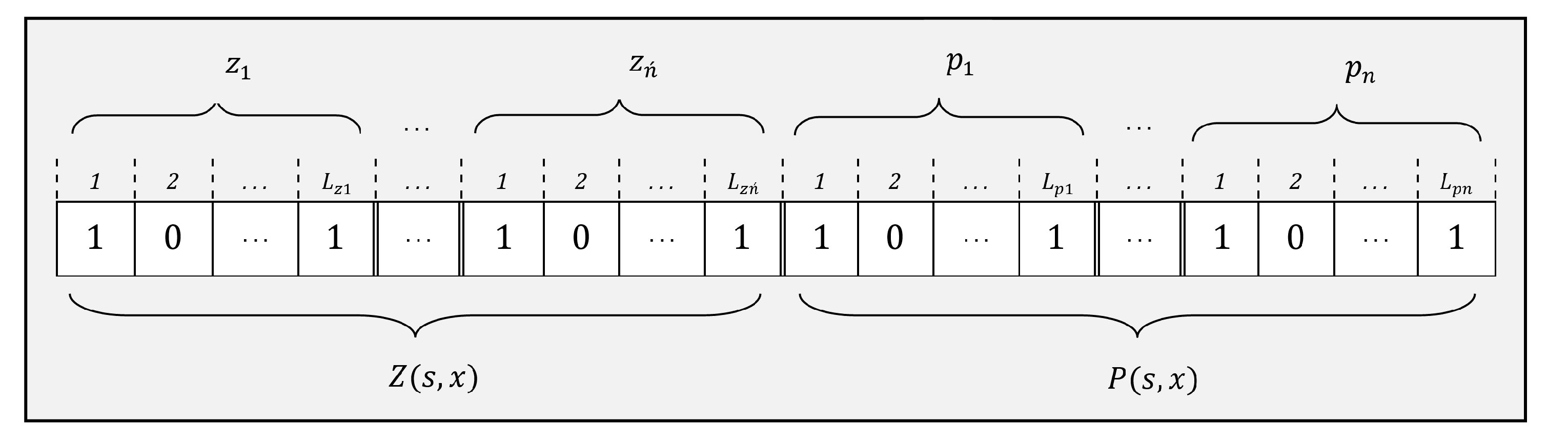
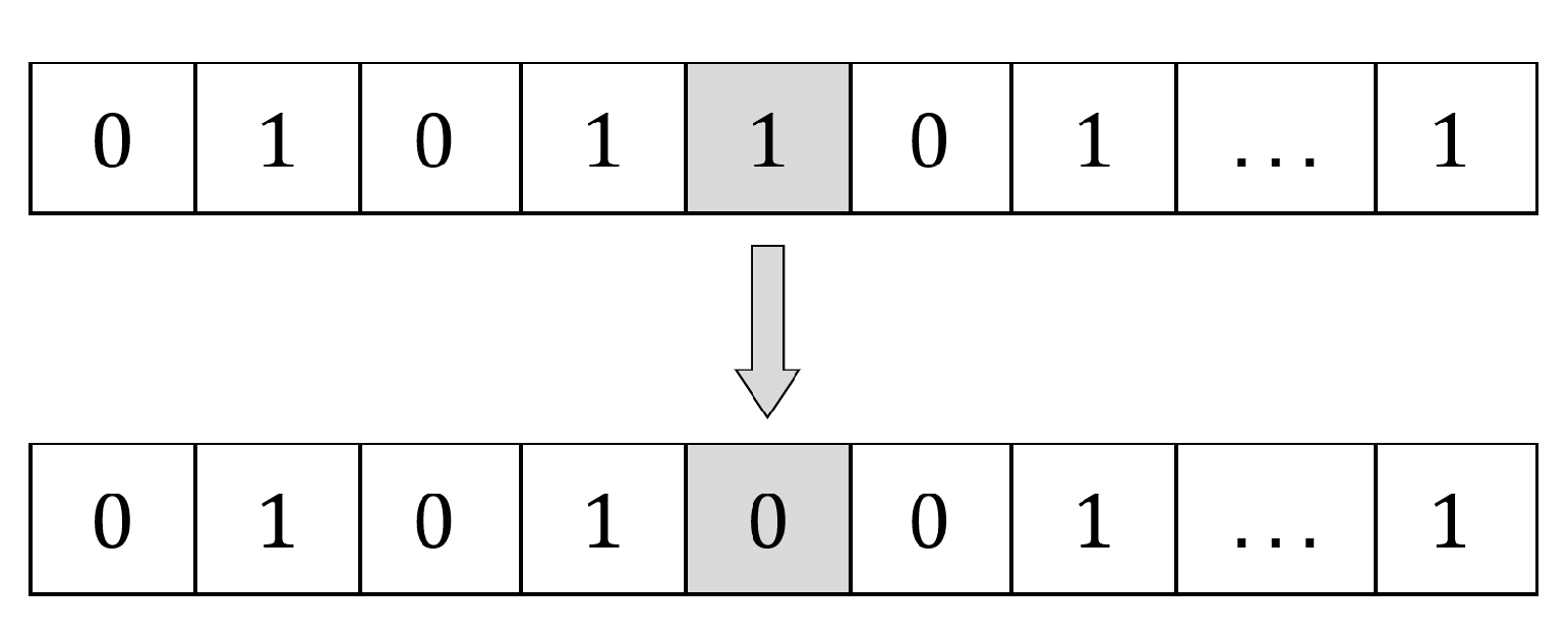
3.2.1. Solution Encoding/Decoding

A possible solution to the pole/zero simplification problem, as shown in Figure 2, is a binary vector of length $L$, where $L$ is the number of original terms, which can be calculated as follows:

$$L=\left(L_{z_1}+L_{z_2}+\cdots +L_{z_{n\prime }}\right)+\left(L_{p_1}+L_{p_2}+\cdots +L_{p_n}\right)={\displaystyle \sum _{j=1}^{n^{\prime }}}{L}_{z_j}+{\displaystyle \sum _{i=1}^n}{L}_{p_i}$$

(34)

where $L_K$, $L_{z_j}$, and $L_{p_i}$ are the number of symbolic terms within the DC-gain $K$, $j$-th zero, and $i$-th pole, respectively.

3.2.2. Generation of the Initial Solution

To construct the initial solution of SA, we utilize heuristic information available in the circuit via a ranking algorithm (RA). This not only improves the convergence speed of SA as it utilizes a near-optimal solution but can also effectively enhance the quality of the final solution. An RA comprises an evaluation step and a selection step. In the first step, each term is eliminated, and accordingly, the generated error rate is measured and stored. After the evaluation of all terms, they are sorted into a list from the best to the worst. In the selection phase, an empty solution is considered, after which the terms within the list are added one by one until all constraints have been satisfied.

3.2.3. Objective Function Evaluation

To evaluate the performance of each solution, an objective function is formulated which compares the simplified pole/zero expressions with the exact ones in terms of the number of terms and mean pole/zero displacements. Moreover, each pole/zero displacement should not exceed the user-specified margin $T_{SA}$. In this direction, the objective function is expressed as a weighted average of three sub-objectives. The first sub-objective (E_n) demonstrates the proportion of the selected symbolic terms to the total number of exact terms extracted by the ERS method. Additionally, the second and third sub-objectives (E_p and E_z) express the mean displacements of the simplified poles and zeroes, respectively. According to Equation (35), these three sub-objectives are merged into a single objective function (OF) to be minimized by the PZSA method, where the sub-objectives E_n, E_p, and E_z are calculated via Equations (36)–(38), respectively.

$$\mathrm{m}\mathrm{i}\mathrm{n}\mathrm{i}\mathrm{m}\mathrm{i}\mathrm{z}\mathrm{e} OF=\left\{w_n{E}_n+w_p{E}_p+w_z{E}_z)\right\}$$

(35)

$$E_n=\frac{1}{L}{\displaystyle \sum _{k=1}^L}{S}_k$$

(36)

$$E_p=\frac{1}{n}{\displaystyle \sum _{i=1}^n}\left(\left|\frac{p_{SA,i}-p_{E,i}}{p_{E,i}}\right|\right)$$

(37)

$$E_z=\frac{1}{n^{\prime }}{\displaystyle \sum _{j=1}^{n^{\prime }}}\left(\left|\frac{z_{SA,j}-z_{E,j}}{z_{E,j}}\right|\right)$$

(38)

subject to:

$$\left|\frac{p_{SA,i}-p_{E,i}}{p_{E,i}}\right|\le T_{SA}\hspace{1em}\hspace{1em}\forall p_{E,i}\in PoleSet$$

(39)

$$\left|\frac{z_{SA,j}-z_{E,j}}{z_{E,j}}\right|\le T_{SA}\hspace{1em}\hspace{1em}\forall z_{E,j}\in ZeroSet$$

(40)

In Equation (35), $w_n$, $w_p$, and $w_z$, are constant parameters ($w_n+w_z+w_z=1$) that specify the relative impacts of the three objectives. As the worst-case pole/zero displacements are limited by Equations (39) and (40), $w_n$ is set as being much larger than $w_p$ and $w_z$ to ensure achieving the simplest expressions.

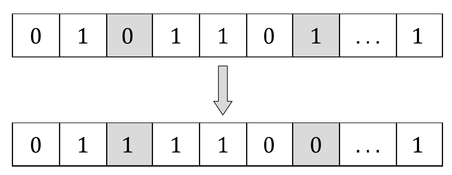
3.2.4. Generation of a New Solution

In each iteration, a neighbor solution, $S^{new}$, is constructed in the vicinity of the current solution, $S^{current}$. We adopt swap (Figure 3) and an exchange (Figure 4) operators as neighborhood search strategies in SA. The reason behind using these operators is to introduce randomness into the optimization process, allowing it to escape from local optima and search for better solutions in the search space. The swap operator adds or removes a term in the exact pole/zero expression, and the exchange operator selects from the available terms while preserving the total number of terms constant. To generate a new solution, an operator is randomly selected with a probability of 50%, and then it operates on the solution $S^{current}$.

3.2.5. Acceptance Rule Checking

In each iteration, if ${OF}^{new}<{OF}^{current}$, the new solution is accepted. Otherwise, if ${OF}^{new}\ge {OF}^{current}$, the new solution (worse solution) has a chance to be accepted with the probability of $P_w$, which can be calculated according to the current temperature $T$ and the differences between the objective function values of the two solutions as follows:

$$P_w=\mathrm{e}\mathrm{x}\mathrm{p}\left(-\frac{E^{new}-E^{current}}{T}\right)$$

(41)

where $T$ is considered to be linearly decreasing during the execution of SA from $T_{initial}$ (initial temperature) to $T_{final}$ (final temperature), as follows:

$$T=T_{initial}+\frac{t}{iter}\left(T_{final}-T_{initial}\right)$$

(42)

4. Performance Evaluation

All simulations are conducted on a PC with a 2.6 GHz CPU and 6 GB RAM. The presented tool has been successfully coded in an MATLAB R2020b m-file running on Windows 10. In order to analyze the performance of the proposed method, we have applied it to three different circuits. All MOS transistors in these circuits are modeled via a small-signal model, as shown in Figure 5. The parameters of the proposed tool have been divided into two categories: Model parameters and SA parameters.

Table 2. Model parameter settings.

Phase	Parameter	Value/Description
Model Parameters	$f_{min}$	1 Hz
	$f_{max}$	10 × $f_T$
	$T_{ERS}$ in Equations (32) and (33)	10%
	$T_{SA}$ in Equations (39) and (40)	20%
	$w_n$ in Equation (35)	0.99
	$w_p$ in Equation (35)	0.005
	$w_z$ in Equation (35)	0.005

provides the selected values for the model parameters. As shown in this table, the model parameters include $f_{min}$, $f_{max}$, $T_{SA}$, $T_{ERS}$, $w_n$, and $w_{pz}$, which engineers should determine based on the desired specifications of the circuit’s application. To perform the experiments in this study, we deploythe typical values for the model parameters which are generally used in the circuit design process. In this regard, the frequency range in which the poles/zeroes are analyzed equals 1 Hz to 10 times the unity gain bandwidth of the active components (10 × $f_T$). The reason for choosing a final frequency of 10 × $f_T$ is to ensure that the circuit response is analyzed up to a frequency where the active components, such as transistors or amplifiers, are still able to provide reasonable gain. At frequencies beyond 10 × $f_T$, the gain of the active components typically drops significantly, and the circuit response may be dominated by the passive components [35]. Additionally, $T_{ERS}$ has been set to 10%, and thus, the poles and zeroes with no more than 10% displacement can be simplified via first-order polynomials, while the other poles and zeroes are expressed via second-order polynomials. Moreover, $T_{SA}$ is selected so that the displacements of the poles/zeroes in the simplified expressions derived by SA are confined to 20%. Eventually, since the maximum displacements of the poles/zeroes are limited by $T_{SA}$, the weight of the term related to the compactness of the symbolic expressions in OF ($w_n$) is set to be much larger than the weight of the average pole/zero displacement ($w_{pz}$). Therefore, the values $w_n$ and $w_{pz}$ are set as 0.99 and 0.01, respectively. As mentioned above, it should be emphasized that the choice of the model parameters depends on the specific circuit and should be modified by the circuit designers according to the application requirements.

Additionally, in the case of the SA parameters, the Taguchi method is utilized to adjust the controllable parameters of SA, comprising maximum iterations, local search operators, $T_{initial}$, and $T_{final}$. In this study, the value of the objective function (OF) is used to evaluate the effectiveness of the algorithm. In order to implement the Taguchi method, we have conducted each experiment 10 times, and the mean and standard deviation values of the objective function are considered as signal and noise values in the Taguchi method, respectively.

Table 3. SA parameter settings using the Taguchi method.

Phase	Parameter	Parameter Levels			Selected Value
SA Parameters	Maximum iterations	L	5 × L	10 × L	5 × L
	Local search operators	Swap	Exchange	Swap/Exchange	Swap/Exchange
	$T_{initial}$ in Equation (42)	10−5	10−4	10−3	10−5
	$T_{final}$ in Equation (42)	0	10−8	10−10	0

presents the analyzed levels for each SA parameter and the optimal level obtained by the Taguchi method.

To justify the proposed methodology, we compare it against a time-constant approach [29], an eigenvalue technique [31], and an evolutionary-based algorithm using a genetic algorithm [26].

4.1. Results for a Three-Stage Amplifier in the RCg_m Model (Circuit 1)

The block diagram of a three-stage compensation OTA is shown in Figure 6. The circuit is described by the RCg_m model. First, the exact expanded TF is derived according to Equation (43) using the MNA technique. Next, by applying the simplification algorithm in [26], the simplified expanded TF is obtained according to Equation (44). By performing PZSA, 3 poles and 2 zeroes can be achieved as Equations (45)–(49).

The comparison of the different methods is summarized in

Table 4. Number of terms within simplified symbolic poles/zeroes in Circuit 1.

Expression	Expanded TF (Exact)	Ref. [26]	Ref. [29]	Ref. [31]	Proposed Exact (ERS)	Proposed Simplified (SA)
P1	-	-	1	10	10	1
P2	-	-	4	26	26	3
P3	-	-	5	25	25	3
Z1	-	-	2	9	3	2
Z2	-	-	2	9	4	2
Overall TF	40	10	-	-	-	-

. According to the obtained results, the exact expanded TF has a total of 40 symbolic terms. The simplification method in [26] obtained an expanded TF according to Equation (44) containing 10 terms. However, even in the simplified form, it cannot give effective insights for the circuit designer to evaluate the positions of the poles and zeroes. By performing the proposed ERS method, 3 poles and 2 zeroes with 10, 26, 25, 3, and 4 terms, resulting in a total of 68 terms, have been extracted. Finally, the proposed PZSA algorithm has reduced the number of terms within these roots to 1, 3, 3, 2, and 2 terms, i.e., totaling 11 terms. Moreover, the numerical results of the different methods are provided in

Table 5. Numerical results for Circuit 1.

Parameter	HSPICE	Expanded TF (Exact)	Ref. [26]	Ref. [29]	Ref. [31]	Proposed Exact	Proposed Simplified
P1 (Hz)	−12.8	−12.8	−13.3	−13.2	−12.8	−12.8	−13.2
P2 (MHz)	−3.19	−3.19	−3.49	−3.19	−2.96	−2.96	−3.18
P3 (MHz)	−40.6	−40.6	−36.3	−43.9	−43.8	−43.8	−39.8
Z1 (MHz)	2.72	2.72	2.72	3.18	3.36	3.18	3.18
Z2 (MHz)	−18.6	−18.6	−18.6	−15.9	−17.5	−15.9	−15.9
Mean pole displacement (%)	-	-	7.8	3.8	5	5	1.9
Max pole displacement (%)	-	-	10.6	8.36	7.9	7.9	3.5
Mean zero displacement (%)	-	-	0.03	15.9	14.7	15.8	15.9
Max zero displacement (%)	-	-	0.04	17.1	23.6	17.1	17.1

, where the last four rows illustrate the error of the simplified equations in terms of the pole and zero displacements when compared to the exact expressions. According to the obtained results, all pole/zero displacements in the derived simplified expressions by the proposed method are less than T_SA = 20%. Although in some cases the existing methods have achieved less pole/zero displacements, the resulting expressions are not as compact as the proposed method. This occurs due to the selection of a much larger value for $w_n$ compared to the values $w_p$ and $w_z$ in the defined objective function. However, as previously mentioned, these values can be modified by the circuit designer based on the desired application requirements.

$$H_E\left(s\right)=\frac{-R_L{R}_{1}G{m}_1\left(\left(C_2{R}_2{C}_{m2}+C_{m1}{R}_2{C}_{m2}\right)s^2-\left(G{m}_2{R}_2{C}_{m1}+C_{m2}\right)s-G{m}_2{R}_{2}G{m}_L\right)}{\begin{array}{c}\left(\begin{array}{l}{C}_{m1}{R}_2{C}_L{R}_L{C}_1{R}_1+C_{m1}{R}_2{C}_L{R}_L{C}_{m2}{R}_1+C_2{R}_2{C}_{m1}{R}_L{C}_{m2}{R}_1+C_2{R}_2{C}_L{R}_L{C}_{m2}{R}_1\\ +C_2{R}_2{C}_{m1}{R}_L{C}_1{R}_1+C_2{R}_2{C}_{m2}{R}_L{C}_1{R}_1+C_{m1}{R}_2{C}_{m2}{R}_L{C}_1{R}_1+C_2{R}_2{C}_L{R}_L{C}_1{R}_1\end{array}\right)s^3\\ +\left(\begin{array}{l}{C}_2{R}_2{C}_{m1}{R}_L+C_{m1}{R}_L{C}_{m2}{R}_1+C_{m1}{R}_2{R}_{L}G{m}_L{C}_1{R}_1-C_{m1}{R}_1{R}_{L}G{m}_2{C}_{m2}{R}_2\\ +C_L{R}_L{C}_1{R}_1+C_2{R}_2{C}_{m2}{R}_1+C_{m1}{R}_L{C}_{m2}{R}_1+C_2{R}_2{C}_1{R}_1+C_{m2}{R}_2{C}_{m1}{R}_1\\ +C_2{R}_2{R}_L{C}_{m2}+C_2{R}_2{R}_L{C}_L+C_{m1}{R}_2{R}_L{C}_{m2}+C_{m1}{R}_2{R}_L{C}_L+C_{m2}{R}_L{C}_1{R}_1\\ +C_{m1}{R}_2{C}_1{R}_1+C_{m1}{R}_2{R}_{L}G{m}_L{C}_{m2}{R}_1+C_L{R}_L{C}_{m2}{R}_1+C_{m1}{R}_L{C}_1{R}_1\end{array}\right)s^2\\ +\left(\begin{array}{l}{R}_L{C}_L+R_L{C}_{m2}+R_L{C}_{m1}+R_2{C}_{m1}+R_2{C}_2+R_1{C}_1\\ +R_1{C}_{m2}+R_1{C}_{m2}{R}_{L}G{m}_2{R}_{2}G{m}_L+C_{m2}{R}_L{R}_{2}G{m}_L\end{array}\right)s+1\end{array}}$$

(43)

$$H_{S,E}\left(s\right)=\frac{-(C_2{R}_1{R}_2{R}_L{C}_{m1}{C}_{m2}+G{m}_1{R}_1{R}_2{R}_L{C}_{m1}{C}_{m2})s^2+\left(G{m}_{1}G{m}_2{R}_1{R}_2{R}_L{C}_{m1}\right)s+G{m}_{1}G{m}_{2}G{m}_L{R}_1{R}_2{R}_L}{\begin{array}{c}\left(C_{m1}{R}_2{C}_L{R}_L{C}_{m2}{R}_1\right)s^3+\left(C_{m1}{R}_2{R}_{L}G{m}_L{C}_1{R}_1+C_{m1}{R}_1{R}_2{R}_{L}G{m}_L{C}_{m2}-C_{m1}{C}_{m2}{R}_1{R}_2{R}_{L}G{m}_2\right)s^2\\ +\left(R_1{C}_{m2}{R}_{L}G{m}_2{R}_{2}G{m}_L\right)s+1\end{array}}$$

(44)

$$P_1=-\frac{1}{R_{1}G{m}_2{R}_{2}G{m}_L{R}_L{C}_{m2}}$$

(45)

$$P_2=-\frac{G{m}_{2}G{m}_L}{C_{m1}(G{m}_L-G{m}_2)}$$

(46)

$$P_3=-\frac{(G{m}_L-G{m}_2)}{C_L}$$

(47)

$$Z_1=\frac{G{m}_L}{C_{m1}}$$

(48)

$$Z_2=-\frac{G{m}_2}{C_{m2}}$$

(49)

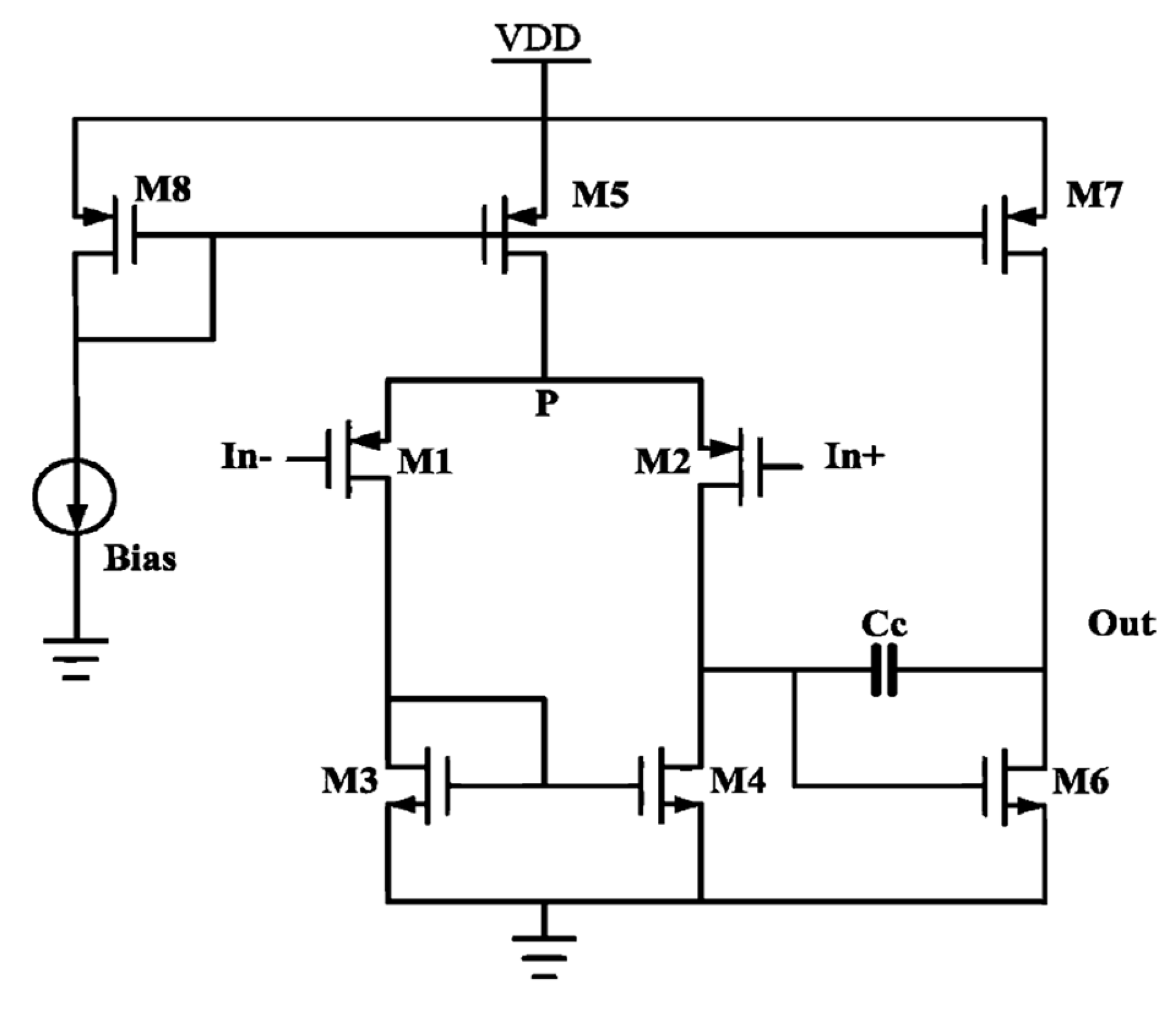
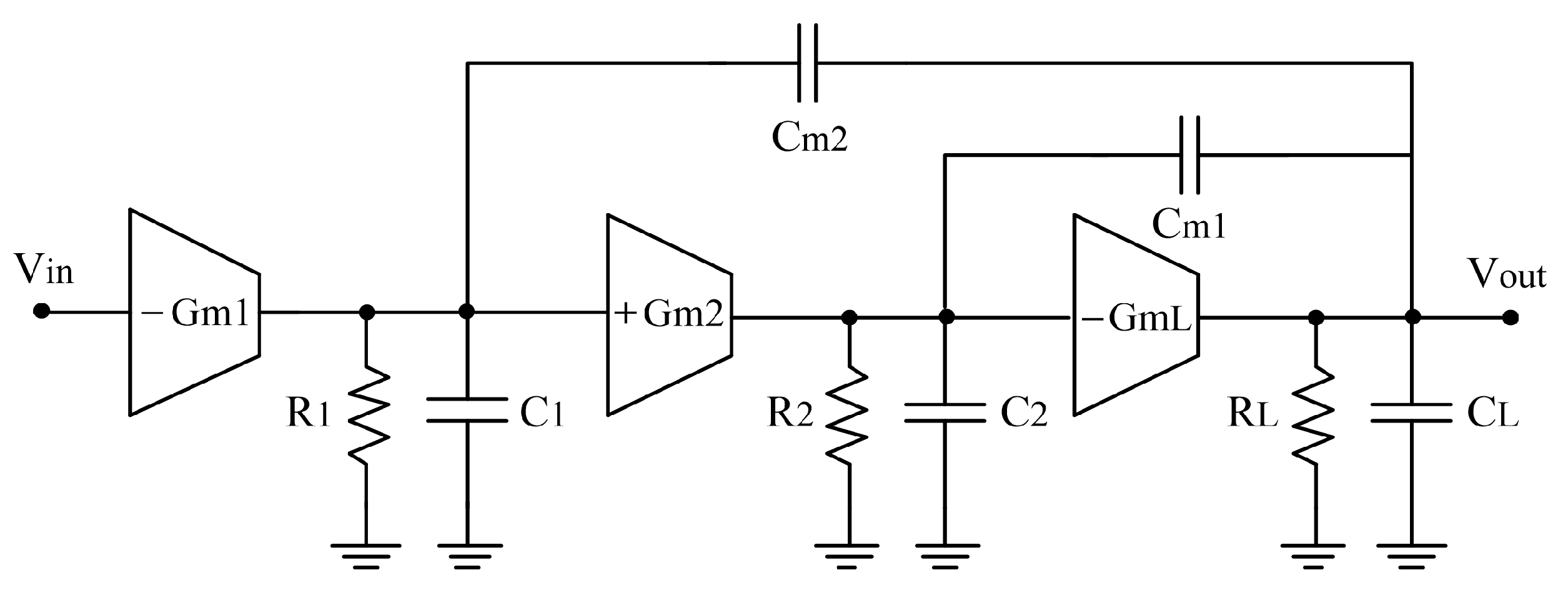
4.2. Results for a Two-Stage Miller Compensated Amplifier (Circuit 2)

The second circuit is a folded cascode two-stage OTA with compensation, as shown in Figure 7. The exact expanded TF obtained by MNA contains 134 symbolic terms. By performing the simplification method outlined in [26], the simplified TF has been obtained according to Equation (50). As shown in

Table 6. Number of terms within the simplified symbolic poles/zeroes in Circuit 2.

Expression	Expanded TF (Exact)	Ref. [26]	Ref. [29]	Ref. [31]	Proposed Exact (ERS)	Proposed Simplified (SA)
P1	-	-	5	104	104	5
P2	-	-	7	82	82	2
Z	-	-	4	18	18	2
Overall TF	134	11	-	-	-	-

, the proposed ERS method has extracted 2 poles and 1 zero with 104, 82, and 18 terms, respectively. Subsequently, the proposed PZSA method has simplified these roots based on Equations (51)–(53), resulting in 5, 2, and 2 terms, respectively. Additionally, a comparison of the numerical results is shown in

Table 7. Numerical results for Circuit 2.

Parameter	HSPICE	Expanded TF (Exact)	Ref. [26]	Ref. [29]	Ref. [31]	Proposed Exact	Proposed Simplified
P1 (KHz)	−177.1	−178.5	−192	−152.8	−178.4	−178.4	−152.8
P2 (MHz)	−377.4	−435.4	−409.1	−341	−435.6	−435.6	−409.3
Z (MHz)	407.2	409.3	409.3	409.3	409.3	409.3	409.3
Mean pole displacement (%)	-	-	6.8	18	0.04	0.04	10.2
Max pole displacement (%)	-	-	7.5	21.7	0.04	0.04	14.4
Zero displacement (%)	-	-	0.01	0.01	0	0	0.01

, which shows that all pole/zero displacements do not exceed T_SA = 20%.

$$H\left(s\right)=\frac{-g_{m1}\left(g_{m1}r{o}_{1}r{o}_{3}r{o}_{6}r{o}_7{C}_c+g_{mb1}r{o}_{1}r{o}_{3}r{o}_{6}r{o}_7{C}_c\right)s+\left(g_{m1}{g}_{m6}r{o}_{1}r{o}_{3}r{o}_{6}r{o}_7+g_{m6}{g}_{mb1}r{o}_{1}r{o}_{3}r{o}_{6}r{o}_7\right)}{\begin{array}{c}r{o}_1\left(g_{m1}r{o}_{3}r{o}_{6}r{o}_7{C}_c{C}_L+g_{mb1}r{o}_{3}r{o}_{6}r{o}_7{C}_c{C}_L\right)s^2+\left(g_{m1}{g}_{m6}r{o}_{3}r{o}_{6}r{o}_7{C}_c+g_{mb1}{g}_{m6}r{o}_{3}r{o}_{6}r{o}_7{C}_c\right)s\\ +\left(g_{m1}r{o}_6+g_{m1}r{o}_7+g_{m1}r{o}_{3}r{o}_7/r{o}_1\right)\end{array}}$$

(50)

$$P_1=-\frac{\left(r{o}_{1}r{o}_6+r{o}_{1}r{o}_7+r{o}_{3}r{o}_6+r{o}_{3}r{o}_7\right)}{g_{m6}r{o}_{1}r{o}_{3}r{o}_{6}r{o}_7{C}_c}=-\frac{1}{g_{m6}\left(r{o}_1‖r{o}_3\right)\left(r{o}_6‖r{o}_7\right)C_c}$$

(51)

$$P_2=-\frac{g_{m6}}{C_L}$$

(52)

$$Z=\frac{g_{m6}}{C_c}$$

(53)

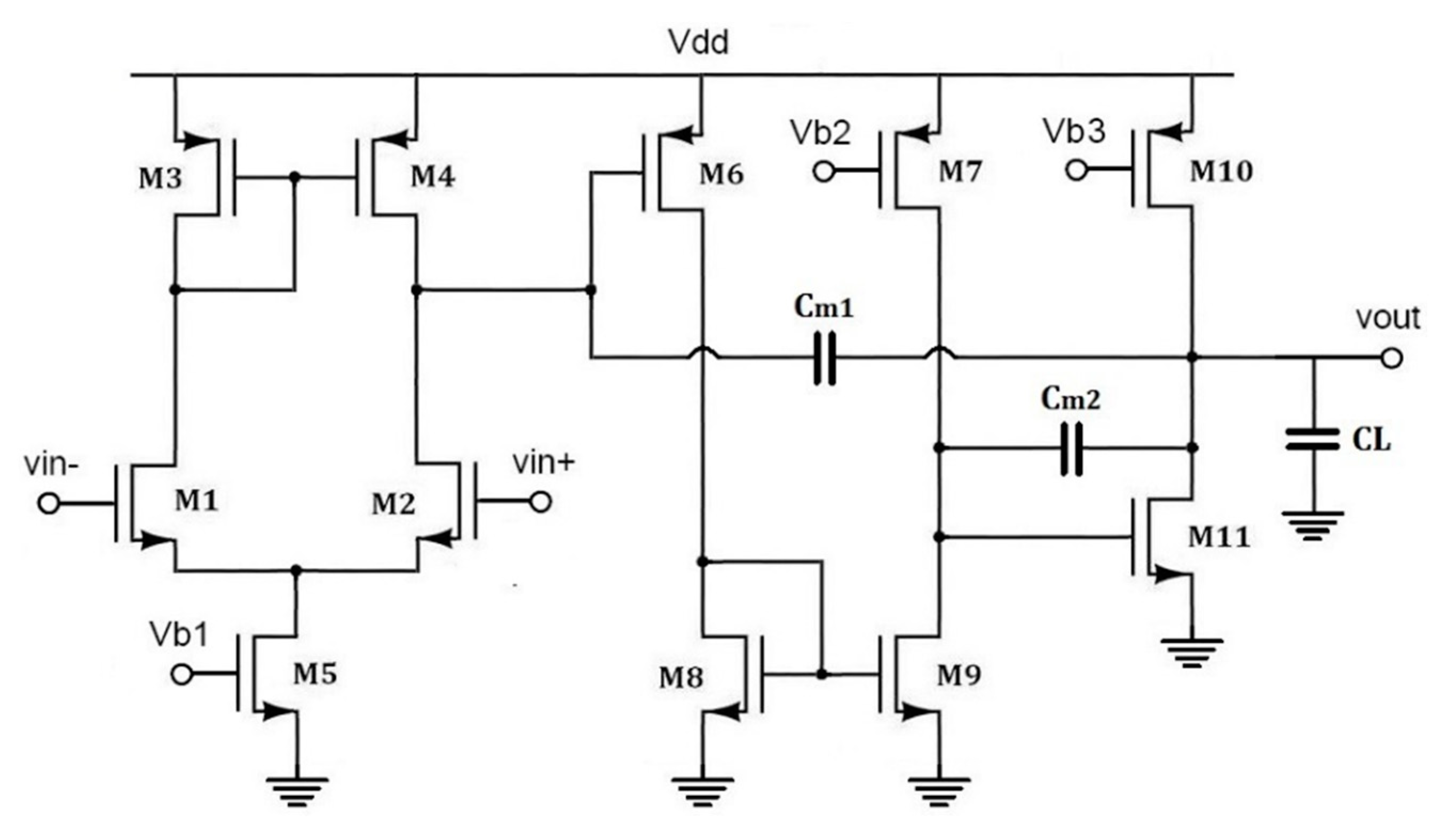
4.3. Results for a Three-Stage Amplifier in Transistor Model (Circuit 3)

The last circuit is a transistor-level three-stage amplifier with miller compensation, as shown in Figure 8. The exact expanded TF of this circuit contains 1320 symbolic terms. Considering the approximation algorithm in [26], the simplified expanded TF with 18 symbolic terms is shown in Equation (54). The ERS method extracted 3 poles and 2 zeroes with a total of 2061 terms. As shown in Equations (55)–(59), applying PZSA to the exact extracted roots reduced them to only a total of 19 terms. The number of simplified terms and numerical results of the different algorithms are summarized in

Table 8. Number of terms within the simplified symbolic poles/zeroes in Circuit 3.

Expression	Expanded TF (Exact)	Ref. [26]	Ref. [29]	Ref. [31]	Proposed Exact (ERS)	Proposed Simplified (SA)
P1	-	-	29	714	714	9
P2	-	-	21	837	837	3
P3	-	-	23	330	330	3
Z1	-	-	15	75	75	2
Z2	-	-	13	105	105	2
Overall TF	1320	18	-	-	-	-

and

Table 9. Numerical results for Circuit 3.

Parameter	HSPICE	Expanded TF (Exact)	Ref. [26]	Ref. [29]	Ref. [31]	Proposed Exact	Proposed Simplified
P1 (Hz)	−27.7	−27.9	−20.6	−20.5	−27.9	−27.9	−22.8
P2 (MHz)	−1.84	−1.84	−2.03	−2.16	−1.76	−1.76	−2.07
P3 (MHz)	−36.6	−40.2	−36.3	−36.1	−42.1	−42.1	−35.7
Z1 (MHz)	1.4	1.4	1.4	2.23	1.62	1.62	1.62
Z2 (MHz)	−10.3	−10.2	−10.5	−7.37	−8.81	−8.81	−9.1
Mean pole displacement (%)	-	-	15.6	18	3	3	14.2
Max pole displacement (%)	-	-	26.4	26.5	4.6	4.6	18.4
Mean zero displacement (%)	-	-	1.7	43.5	14.8	14.8	13.5
Max zero displacement (%)	-	-	2.9	59.3	15.9	15.9	16.1

, respectively.

$$H(s)=\frac{\begin{array}{c}-\left(g_{m1}{g}_{m8}r{o}_{1}r{o}_{3}r{o}_{6}r{o}_{7}r{o}_{8}r{o}_{9}r{o}_{10}r{o}_{11}{C}_{m1}{C}_{m2}\right)s^2-\left(g_{m1}{g}_{m6}{g}_{m9}r{o}_{1}r{o}_{3}r{o}_{6}r{o}_{7}r{o}_{8}r{o}_{9}r{o}_{10}r{o}_{11}{C}_{m2}\right)s\\ +g_{m1}{g}_{m6}{g}_{m9}{g}_{m11}r{o}_{1}r{o}_{3}r{o}_{6}r{o}_{7}r{o}_{8}r{o}_{9}r{o}_{10}r{o}_{11}\end{array}}{\begin{array}{c}\left(\begin{array}{l}{g}_{m8}r{o}_{1}r{o}_{6}r{o}_{7}r{o}_{8}r{o}_{10}+g_{m8}r{o}_{3}r{o}_{6}r{o}_{8}r{o}_{9}r{o}_{10}+g_{m8}r{o}_{1}r{o}_{6}r{o}_{8}r{o}_{9}r{o}_{10}+g_{m8}r{o}_{3}r{o}_{6}r{o}_{8}r{o}_{9}r{o}_{11}\\ +g_{m8}r{o}_{3}r{o}_{6}r{o}_{7}r{o}_{8}r{o}_{10}+g_{m8}r{o}_{1}r{o}_{6}r{o}_{7}r{o}_{8}r{o}_{11}+g_{m8}r{o}_{3}r{o}_{6}r{o}_{7}r{o}_{8}r{o}_{11}+g_{m8}r{o}_{1}r{o}_{6}r{o}_{8}r{o}_{9}r{o}_{11}\end{array}\right)\\ +\left(g_{m8}r{o}_{1}r{o}_{3}r{o}_{6}r{o}_{7}r{o}_{8}r{o}_{9}r{o}_{10}r{o}_{11}{C}_{m1}{C}_{m2}{C}_L\right)s^3+\left(g_{m6}{g}_{m9}{g}_{m11}r{o}_{1}r{o}_{3}r{o}_{6}r{o}_{7}r{o}_{8}r{o}_{9}r{o}_{10}r{o}_{11}{C}_{m1}\right)s\\ +\left(\begin{array}{l}{g}_{m8}r{o}_{1}r{o}_{3}r{o}_{6}r{o}_{7}r{o}_{8}r{o}_{9}r{o}_{10}{C}_{m1}{C}_{m2}-g_{m6}{g}_{m9}r{o}_{1}r{o}_{3}r{o}_{6}r{o}_{7}r{o}_{8}r{o}_{9}r{o}_{10}r{o}_{11}{C}_{m1}{C}_{m2}\\ +g_{m11}r{o}_{1}r{o}_{3}r{o}_{7}r{o}_{8}r{o}_{9}r{o}_{10}r{o}_{11}{C}_{m1}{C}_{m2}+g_{m11}r{o}_{1}r{o}_{3}r{o}_{6}r{o}_{7}r{o}_{9}r{o}_{10}r{o}_{11}{C}_{m1}{C}_{m2}\\ +g_{m8}{g}_{m11}r{o}_{1}r{o}_{3}r{o}_{6}r{o}_{7}r{o}_{8}r{o}_{9}r{o}_{10}r{o}_{11}{C}_{m1}{C}_{m2}\end{array}\right)s^2\end{array}}$$

(54)

$$P_1=-\frac{g_{m8}(r{o}_1+r{o}_3)(r{o}_7+r{o}_9)(r{o}_{10}+r{o}_{11})}{g_{m6}{g}_{m9}{g}_{m11}r{o}_{1}r{o}_{3}r{o}_{7}r{o}_{9}r{o}_{10}r{o}_{11}{C}_{m1}}=-\frac{g_{m8}}{g_{m6}{g}_{m9}{g}_{m11}{C}_{m1}\left(r{o}_1‖r{o}_3\right)\left(r{o}_7‖r{o}_9\right)\left(r{o}_{10}‖r{o}_{11}\right)}$$

(55)

$$P_2=-\frac{g_{m6}{g}_{m9}{g}_{m11}}{\left(g_{m8}{g}_{m11}-g_{m6}{g}_{m9}\right)C_{m2}}$$

(56)

$$P_3=-\frac{\left(g_{m8}{g}_{m11}-g_{m6}{g}_{m9}\right)}{g_{m8}{C}_L}$$

(57)

$$Z_1=\frac{g_{m11}}{C_{m2}}$$

(58)

$$Z_2=-\frac{g_{m6}{g}_{m9}}{g_{m8}{C}_{m1}}$$

(59)

4.4. Discussion

Generally, in the reported simplified symbolic pole/zero expressions, three types of errors can be observed:

Error-1: the first type of error may occur by comparing HSPICE with the exact expanded TF achieved by MNA. This error may be observed for OTAs described at the transistor level, as HSPICE considers a more accurate small-signal transistor model than the simple model in our program.

Error-2: the second type of error may be observed when comparing the exact TF with the exact extracted poles/zeroes because of the simplifications induced by the root extraction process in the ERS method.

Error-3: the third error may occur between exact pole/zero expressions and the simplified ones due to the simplifications done by PZSA.

As mentioned above, Error-1 is inevitable in symbolic analysis, which is observed in all symbolic tools. However, Error-2 and Error-3 may occur because of our pole/zero extraction and simplification methods, respectively. Therefore, in the results shown in Table 5, Table 7 and Table 9, we have reported these errors for each algorithm by comparing them with the exact expanded TF. Thus, the numerical results of the poles and zeroes in the exact TF were considered as references to justify the performance of the different techniques.

Table 10. Sub-objective values for different circuits.

Circuit/Objective	En	Ep	Ez
Circuit 1	0.1617	0.019	0.159
Circuit 2	0.0441	0.102	0.0001
Circuit 3	0.0092	0.142	0.135

reports the obtained values of the three sub-objectives (E_n, E_p, and E_z) for the different circuits. As previously mentioned, the total number of terms in the exact poles/zero expressions extracted by the ERS method are 68, 204, and 2061 for circuits 1, 2, and 3, respectively. Subsequently, these expressions are then simplified by the PZSA method resulting in a total of 11, 9, and 19 terms. As a result, the first sub-objective (E_n) equals the proportion of the number of simplified terms to the exact terms for each circuit. Additionally, the obtained results for the sub-objectives E_p and E_z demonstrate that all pole/zero displacements do not exceed the pre-specified threshold of T_SA = 20%.

In addition, since SA is a non-deterministic algorithm that produces different results in each run, its performance was assessed by running it on each circuit 10 times. The resulting objective function values and their average and standard deviation are summarized in

Table 11. Overall objective function values in 10 successive runs for different circuits.

Circuit/Objective	Circuit 1	Circuit 2	Circuit 3
Run 1	0.1619	0.0447	0.0119
Run 2	0.162	0.0451	0.013
Run 3	0.1618	0.0448	0.0128
Run 4	0.1766	0.045	0.0123
Run 5	0.162	0.0447	0.0114
Run 6	0.1767	0.0445	0.0115
Run 7	0.1617	0.0446	0.012
Run 8	0.1616	0.0449	0.0129
Run 9	0.1473	0.0398	0.0117
Run 10	0.1621	0.0447	0.0121
Average	0.1634	0.0443	0.0122
Standard Deviation	0.0083	0.0016	0.0006

. According to the obtained results, the proportion of the standard deviation to the average values equals 5.1%, 3.6%, and 4.7% for circuits 1, 2, and 3, respectively, which demonstrates the robustness of the proposed PZSA.

5. Conclusions

This paper presented a mathematical technique for symbolic circuit pole/zero extraction, followed by a combined heuristic–metaheuristic algorithm to simplify the extracted expressions. In the proposed method, a mathematical model was presented for extracting the exact poles and zeroes from the original expanded expression of OTA. Then, an ensemble heuristic–metaheuristic approach was proposed to obtain the simplest symbolic pole/zero equations from the exact ones. In the proposed ensemble method, a near-optimal solution was constructed using the knowledge-based heuristic information available in the circuit model. Subsequently, a metaheuristic algorithm based on simulated annealing was used to obtain the simplest pole/zero expressions with the best achievable quality. The proposed tool has been coded in an m-file of MATLAB to extract simplified pole/zero equations directly from the circuit netlist. Simulations on three OTAs demonstrated the effectiveness and superiority of the proposed technique against the existing algorithms in the literature.

Besides the advantages mentioned above, the proposed method has some limitations that can be addressed in future studies. The proposed methodology relies on a single nominal point for the circuit parameters, and thus, the simplified root expressions are valid around the nominal point. As a future work, the proposed method can be extended to deal with the uncertainties of the circuit parameters using robust optimization techniques, Monte Carlo simulation, fuzzy arithmetic, etc. Another limitation of this study is that the suggested method is a simplification-after-generation technique, in which the symbolic expressions should be generated exactly before the simplification process. Since circuit simplification is an NP-hard problem, the computational complexity of the exact expressions increases exponentially with the circuit size. Thus, the use of metaheuristic algorithms is challenging for large-size circuits from the time complexity point of view. As an interesting future research direction, the proposed method can be hybridized with simplification-before-generation approaches to deal with larger circuits. Moreover, we suggest performing other metaheuristics and their hybridizations with other soft computing techniques [36,37] in order to solve the root simplification problem.

References

1. Gielen, G.; Sansen, W.M. Symbolic Analysis for Automated Design of Analog Integrated Circuits; Springer Science + Business Media: Berlin, Germany, 2012; Volume 137. [Google Scholar]
2. Riad, J.; Soto-Aguilar, S.; Estrada-López, J.J.; Moreira-Tamayo, O.; Sánchez-Sinencio, E. Design Trade-Offs in Common-Mode Feedback Implementations for Highly Linear Three-Stage Operational Transconductance Amplifiers. Electronics 2021, 10, 991. [Google Scholar] [CrossRef]
3. Akbari, M.; Shokouhifar, M.; Hashemipour, O.; Jalali, A.; Hassanzadeh, A. Systematic design of analog integrated circuits using ant colony algorithm based on noise optimization. Analog. Integr. Circuits Signal Process. 2016, 86, 327–339. [Google Scholar] [CrossRef]
4. Rodovalho, L.H.; Toledo, P.; Mir, F.; Ebrahimi, F. Hybrid Inverter-Based Fully Differential Operational Transconductance Amplifiers. Chips 2023, 2, 1–19. [Google Scholar] [CrossRef]
5. Akbari, M.; Hussein, S.M.; Hashim, Y.; Khateb, F.; Kulej, T.; Tang, K.T. Implementation of a Multipath Fully Differential OTA in 0.18-μm CMOS Process. IEEE Trans. Very Large Scale Integr. (VLSI) Syst. 2022, 31, 147–151. [Google Scholar] [CrossRef]
6. Aminzadeh, H.; Grasso, A.D.; Palumbo, G. A methodology to derive a symbolic transfer function for multistage amplifiers. IEEE Access 2022, 10, 14062–14075. [Google Scholar] [CrossRef]
7. Shokouhifar, M.; Jalali, A. Simplified symbolic transfer function factorization using combined artificial bee colony and simulated annealing. Appl. Soft Comput. 2017, 55, 436–451. [Google Scholar] [CrossRef]
8. Grasso, A.D.; Marano, D.; Pennisi, S.; Vazzana, G. Symbolic factorization methodology for multistage amplifier transfer functions. Int. J. Circuit Theory Appl. 2015, 44, 38–59. [Google Scholar] [CrossRef]
9. Shi, G.; Tan, S.X.D.; Tlelo-Cuautle, E. Advanced Symbolic Analysis for VLSI Systems; Springer: Berlin, Germany, 2014. [Google Scholar]
10. Shokouhifar, M.; Jalali, A. An evolutionary-based methodology for symbolic simplification of analog circuits using genetic algorithm and simulated annealing. Expert Syst. Appl. 2015, 42, 1189–1201. [Google Scholar] [CrossRef]
11. Shokouhifar, M.; Jalali, A. Simplified symbolic gain, CMRR and PSRR analysis of analog amplifiers using simulated annealing. J. Circuits Syst. Comput. 2016, 25, 1650082. [Google Scholar] [CrossRef]
12. Sathasivam, S.; Mamat, M.; Kasihmuddin, M.S.M.; Mansor, M.A. Metaheuristics approach for maximum k satisfiability in restricted neural symbolic integration. Pertanika J. Sci. Technol. 2020, 28, 545–564. [Google Scholar]
13. Ali, S.; Bhargava, A.; Saxena, A.; Kumar, P. A Hybrid Marine Predator Sine Cosine Algorithm for Parameter Selection of Hybrid Active Power Filter. Mathematics 2023, 11, 598. [Google Scholar] [CrossRef]
14. Dziedziewicz, S.; Warecka, M.; Lech, R.; Kowalczyk, P. Self-Adaptive Mesh Generator for Global Complex Roots and Poles Finding Algorithm. IEEE Trans. Microw. Theory Tech. 2023, 66, 7198–7205. [Google Scholar] [CrossRef]
15. Kirkpatrick, S.; Gelatt, C.D.; Vecchi, M.P. Optimization by Simulated Annealing. Science 1983, 220, 671–680. [Google Scholar] [CrossRef] [PubMed]
16. Hennig, E. Symbolic Approximation and Modeling Techniques for Analysis and Design of Analog Circuits; Shaker Verlag: Herzogenrath, Germany, 2000. [Google Scholar]
17. Toumazou, C.; Moschytz, G.S.; Gilbert, B. Trade-Offs in Analog Circuit Design: The Designer’s Companion; Kluwer Academic Publishers: New York, NY, USA, 2014. [Google Scholar]
18. Wierzba, G.; Srivastava, A.; Joshi, V.; Noren, K.; Svoboda, J. SSPICE-A symbolic SPICE program for linear active circuits. Midwest Symp. Circuits Syst. 1989, 2, 1197–1201. [Google Scholar]
19. Fernández, F.V.; Rodríguez-Vázquez, A.; Huertas, J.L. Interactive AC modeling and characterization of analog circuits via symbolic analysis. Kluwer J. Analog. Integr. Circuits Signal Process. 1991, 1, 183–208. [Google Scholar]
20. Gielen, G.; Walscharts, H.; Sansen, W. ISAAC: A symbolic simulator for analog integrated circuits. IEEE J. Solid-State Circuits 1989, 24, 1587–1597. [Google Scholar] [CrossRef]
21. Fakhfakh, M.; Cuautle, E.T.; Fernandez, F.V. Design of Analog Circuits through Symbolic Analysis; Bentham Science Publishers: Sharjah, United Arab Emirates, 2012. [Google Scholar]
22. Shokouhifar, M.; Jalali, A. Automatic Simplified Symbolic Analysis of Analog Circuits Using Modified Nodal Analysis and Genetic Algorithm. J. Circuits Syst. Comput. 2015, 24, 1–20. [Google Scholar] [CrossRef]
23. Shokouhifar, M.; Jalali, A. Evolutionary based simplified symbolic PSRR analysis of analog integrated circuits. Analog. Integr. Circuits Signal Process. 2016, 86, 189–205. [Google Scholar] [CrossRef]
24. Panda, M.; Kumar Patnaik, S.; Kumar Mal, A.; Ghosh, S. Fast and optimised design of a differential VCO using symbolic technique and multi objective algorithms. IET Circuits Devices Syst. 2019, 13, 1187–1195. [Google Scholar] [CrossRef]
25. Panda, M.; Patnaik, S.K.; Mal, A.K. An efficient method to compute simplified noise parameters of analog amplifiers using symbolic and evolutionary approach. Int. J. Numer. Model. Electron. Netw. Devices Fields 2021, 34, e2790. [Google Scholar] [CrossRef]
26. Zhou, R.; Poechmueller, P.; Wang, Y. An Analog Circuit Design and Optimization System with Rule-Guided Genetic Algorithm. IEEE Trans. Comput.-Aided Des. Integr. Circuits Syst. 2022, 41, 5182–5192. [Google Scholar] [CrossRef]
27. Hayes, M. Lcapy: Symbolic linear circuit analysis with Python. PeerJ Comput. Sci. 2022, 8, e875. [Google Scholar] [CrossRef] [PubMed]
28. Guerra, O.; Rodriguez-Garcia, J.D.; Fernandez, F.V.; Rodríguez-Vázquez, A. A symbolic pole/zero extraction methodology based on analysis of circuit time-constants. Analog. Integr. Circuits Signal Process. 2002, 31, 101–118. [Google Scholar] [CrossRef]
29. Gomes, J.L.; Nunes, L.C.; Gonçalves, C.F.; Pedro, J.C. An accurate characterization of capture time constants in GaN HEMTs. IEEE Trans. Microw. Theory Tech. 2019, 67, 2465–2474. [Google Scholar] [CrossRef]
30. Cao, H.; Zhang, Y.; Han, Z.; Shao, X.; Gao, J.; Huang, K.; Shi, Y.; Tang, J.; Shen, C.; Liu, J. Temperature compensation circuit design and experiment for dual-mass MEMS gyroscope bandwidth expansion. IEEE/ASME Trans. Mechatron. 2019, 24, 677–688. [Google Scholar] [CrossRef]
31. Coşkun, K.Ç.; Hassan, M.; Drechsler, R. Equivalence Checking of System-Level and SPICE-Level Models of Linear Circuits. Chips 2022, 1, 54–71. [Google Scholar] [CrossRef]
32. Evnin, O. Melonic dominance and the largest eigenvalue of a large random tensor. Lett. Math. Phys. 2021, 111, 66. [Google Scholar] [CrossRef]
33. Gheorghe, A.G.; Constantinescu, F. Pole/Zero Computation for Linear Circuits. In Proceedings of the 2012 Sixth UKSim/AMSS European Symposium on Computer Modeling and Simulation, Valletta, Malt, 14–16 November 2012; pp. 477–480. [Google Scholar]
34. Sohrabi, M.; Zandieh, M.; Shokouhifar, M. Sustainable inventory management in blood banks considering health equity using a combined metaheuristic-based robust fuzzy stochastic programming. Socio-Econ. Plan. Sci. 2022, 86, 101462. [Google Scholar] [CrossRef]
35. Razavi, B. Fundamentals of Microelectronics; John Wiley & Sons: New York, NY, USA, 2021. [Google Scholar]
36. Ghasemi Darehnaei, Z.; Shokouhifar, M.; Yazdanjouei, H.; Rastegar Fatemi, S.M.J. SI-EDTL: Swarm intelligence ensemble deep transfer learning for multiple vehicle detection in UAV images. Concurr. Comput. Pract. Exp. 2022, 34, e6726. [Google Scholar] [CrossRef]
37. Aziz, R.M.; Mahto, R.; Goel, K.; Das, A.; Kumar, P.; Saxena, A. Modified Genetic Algorithm with Deep Learning for Fraud Transactions of Ethereum Smart Contract. Appl. Sci. 2023, 13, 697. [Google Scholar] [CrossRef]
Figure 1. Overall flowchart of the proposed methodology.
Mathematics 11 01498 g001
Figure 2. Encoding of a solution: If S i = 1, the i -th symbolic term is present in the solution; otherwise, if S i = 0, the i -th term has been discarded from the solution.
Mathematics 11 01498 g002
Figure 3. Swap: a symbolic term is randomly selected and inverted.
Mathematics 11 01498 g003
Figure 4. Exchange: a term “0” and a term “1” are randomly selected and exchanged.
Mathematics 11 01498 g004
Figure 5. Small signal representation of MOS transistors.
Mathematics 11 01498 g005
Figure 6. A three-stage amplifier in the RCgm model.
Mathematics 11 01498 g006
Figure 7. Two-stage compensation amplifier.
Mathematics 11 01498 g007
Figure 8. A three-stage amplifier in the transistor model.
Mathematics 11 01498 g008