Scheduling of Software Test to Minimize the Total Completion Time ^†

Abstract

This paper investigates a single-machine scheduling problem of a software test with shared common setup operations. Each job has a corresponding set of setup operations, and the job cannot be executed unless its setups are completed. If two jobs have the same supporting setups, the common setups are performed only once. No preemption of any processing is allowed. This problem is known to be computationally intractable. In this study, we propose sequence-based and position-based integer programming models and a branch-and-bound algorithm for finding optimal solutions. We also propose an ant colony optimization algorithm for finding approximate solutions, which will be used as the initial upper bound of the branch-and-bound algorithm. The computational experiments are designed and conducted to numerically appraise all of the proposed methods.

1. Introduction

Scheduling is the decision-making process used by many manufacturing and service industries to allocate resources to economic activities or tasks over he planning horizon [1,2]. This paper studies a scheduling model that is inspired by real-life applications, where supporting operations need to be prepared before regular jobs are processed. The specific application context is the scheduling of asoftware test at an IC design company, where the software system is modular and can be tested module by module and level by level. Before starting a module test, we need to install software utilities and libraries as well as adjust system parameters to shape an appropriate system environment. The setup operation corresponds to the installation of utilities and libraries, which are supporting tasks for the job. Different tests may require part of the same environment settings. If two jobs have common supporting tasks, the common setups are performed only once. The abstract model was also studied by Kononov, Lin, and Fang [3] as a single-machine scheduling problem formulated from the production scheduling of multimedia works. In the context of multimedia scheduling, when we want to play multimedia, we need to download their content first, including audio tracks, subtitles, and images, which can correspond to setup operations and jobs for this study, respectively. Once the setup operations of the multimedia objects are prepared, they can be embedded in upper-level objects without multiple copies, as in physical products. This unique property is different from the manufacture of tangible products, such as vehicles and computers. Following the standard three-field notation [4], we denote the model by $1|bp-prec|{\sum }_j{C}_j$, where the one indicates the single-machine setting, $bp-prec$ indicates the bipartite precedence relation between shared setups and test jobs, and ${\sum }_j{C}_j$ is the objective to minimize the total completion time.

This paper is organized into seven sections. In Section 2, the problem definition is presented with a numerical example for illustrations. The literature review follows. Section 3 introduces two integer programming models based on different formulation approaches. Section 4 is dedicated to the development of a branch-and-bound algorithm, including the development of upper bound, lower bound, and tree traversal methods. In Section 5, an ant colony optimization algorithm is proposed. Section 6 presents the computational experiments on the proposed methods. Finally, conclusions and suggestions for future works are given in Section 7.

2. Problem Definition and Literature Review

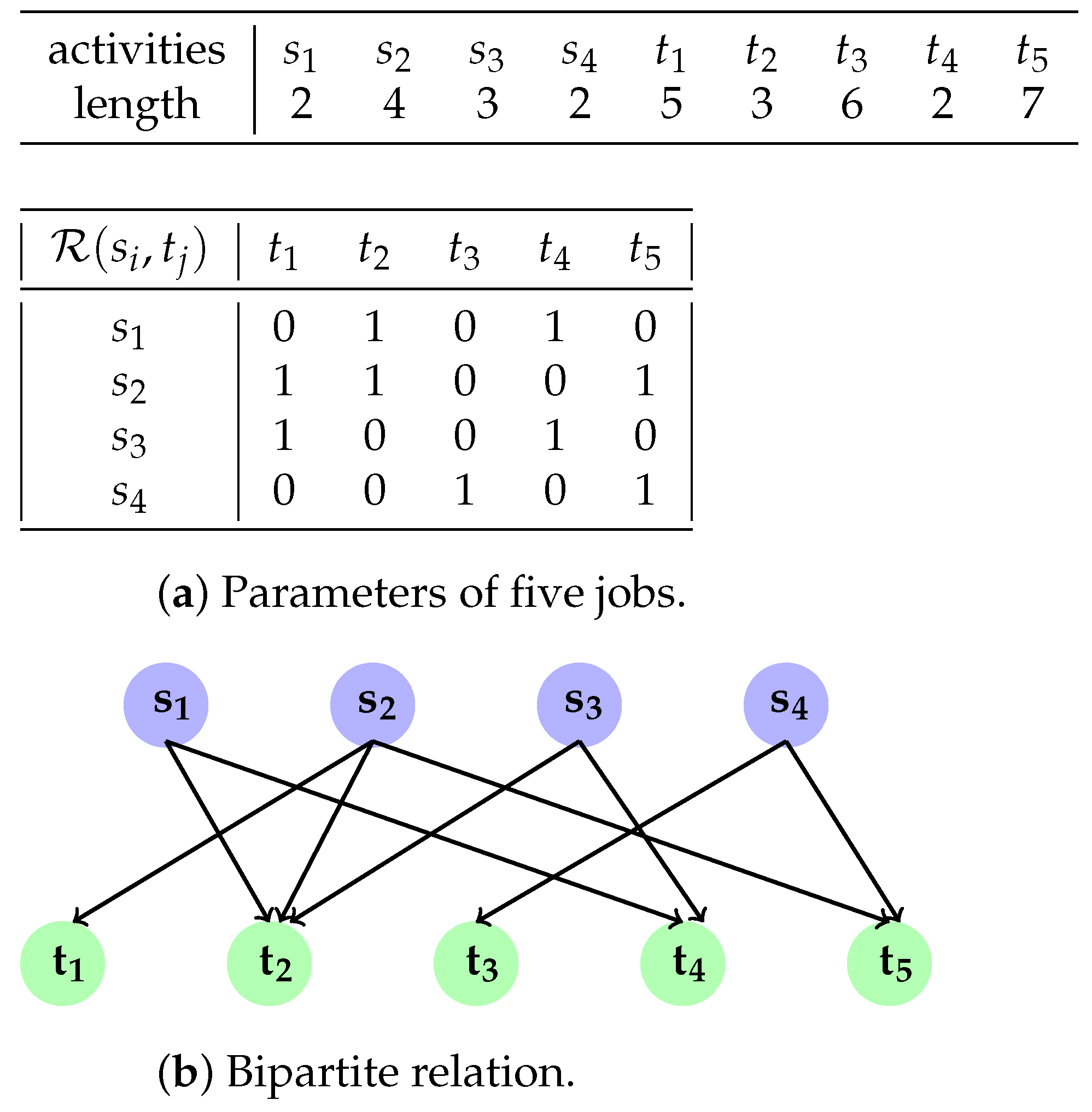
2.1. Problem Statements

We first present the notation that will be used in this paper. Note that all parameters are assumed to be non-negative integers.

n	number of jobs;
m	number of setup operations;
$T=\{t_1,t_2,\dots ,t_n\}$	set of jobs to be processed;
$S=\{s_1,s_2,\dots ,s_m\}$	set of setup operations;
$\mathcal{R}=\left\{(s_i,t_j)\right|s_i\in Ssupports{t}_j\in T\}$	relation indicating whether the setup operation $s_i$
	is required for each job $t_j$;
$p_j$	processing time of job $t_j$ on the machine;
$s{p}_i$	processing time of setup $s_i$ on the machine;
$\sigma =({\sigma }_1,{\sigma }_2,\dots ,{\sigma }_n)$	particular sequence of the jobs;
${\sigma }^{\ast }$	optimal schedule sequence;
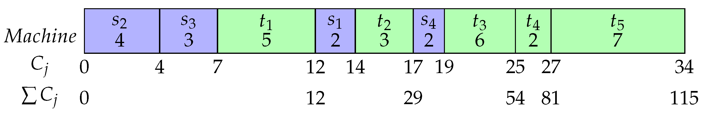
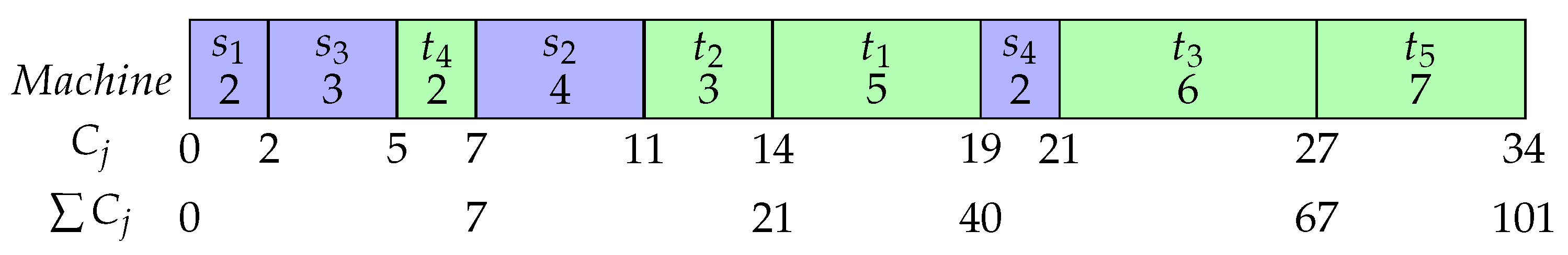
$C_j$	completion time of job $t_j$;
$Z\left(\sigma \right)={\sum }_{j\in T}$	total job completion time under schedule $\sigma$.

The subject of our research is dedicated to studying the single-machine scheduling problem with shared common setup operations. The objective is to minimize the total completion time of the jobs, i.e., $\Sigma C_j$. The problem can be described as follows:

From time zero onwards, two disjoint sets of activities S and T are to be processed on a machine. Each job $t_j$ has a set of setup operations that job $t_j$ can only start after its setups are completed. All setup operations and jobs can be performed on the machine at any time. Although all setup operations need to be processed once, they do not contribute to the objective function because their role is only the preparatory operations for jobs under the priority relation. At any time, the machine can process at most one setup operation or job. No preemption of any processing is allowed. In software test scheduling, jobs $t_j$ represent the software to be tested, and setups $s_i$ refers to the preparation of a programming language or compilation environment that needs to be installed in advance so that the test software can be executed. For example, if $t_1$ is an Android application that needs to be tested, and $t_1$ needs setups $s_1$ and $s_4$, then $s_1$ could be JAVA, $s_4$ could be Android Studio, etc.

To illustrate the problem of our study, we give numerical examples of four setup operations, five test jobs, the relation $\mathcal{R}$, and its corresponding graph. The parameters and relation are shown in Figure 1.

Two example schedules are produced and shown below in the form of Gantt charts. The feasible schedule shown in Figure 2 is $\sigma =(t_1,t_2,t_3,t_4,t_5)$ with a total completion time of 115. Setups $s_2,s_3$ precede job $t_1$. The order of $s_2$ and $s_3$ is immaterial. Figure 3 shows schedule ${\sigma }^{\ast }=(t_4,t_2,t_1,t_3,t_5)$ associated with a total completion time of 101, which is optimal for the given instance. While both are feasible solutions, the objective value of Figure 3 will be better than that of Figure 2.

2.2. Literature Review

The scheduling problem studied by Kononov, Lin, and Fang [3] has a single machine that performs all setup operations and testing jobs. Referring to Brucker [5] and Leung [1], we know that precedence constraints play a crucial role in scheduling problems, especially when complexity status or categories are involved. Existing research works in the literature consider precedence relations presented in various forms. Bipartite graphs are often studied in graph theory. The graph shown in Figure 1 is bipartite because edges exist between nodes on one side and nodes on the other. Linear allocation problems can also be visualized by both supply and demand. Unfortunately, scheduling theory rarely addresses precedence constraints in bipartite graphs.

After formulation, Kononov, Lin, and Fang [3] studied two minimum sum objective functions, namely the number of late jobs and the total weighted completion time of jobs. As for the minimization of the total weighted completion time (${\sum }_j{w}_j{C}_j$), Baker [6] is probably the first paper to address the existence of precedence constraints. Adolphson and Hu [7] proposed a polynomial time algorithm for the case in which rooted trees give priority. A fundamental problem for the jobs-per-unit execution time is $1|prec,p_i=1|\sum w_j{C}_j$, where $w_j\in 1,2,3$ has been proven to be strongly NP-hard by Lawler [8]. The minimum latency set cover problem studied by Hassin and Levin [9] is the most relevant. The minimum latency set cover problem involves a subset of several operations. A subset is complete when all of their operations are finished. The objective function is the total weighted completion time of subsets. The minimum latency set cover problem is a special case of our $1|bp-prec|\sum w_j{C}_j$ problem, and the correspondence is as follows: In our problem, an operation is mapped to a setup operation ($s_i$), and a subset is interpreted as a testing job ($t_j$). Furthermore, Hassin and Levin [9] showed that the minimum delay set cover problem is strongly NP-hard even if all operations require the unit execution time (UET). Subsequently, the $1|bp-prec|\sum w_j{C}_j$ problem is hard as well. By performing a pseudo-polynomial time reduction in Lawler’s result about $1|prec,p_j=1|\sum w_j{C}_j$, where $w_j\in 1,2,3$, Kononov, Lin, and Fang [3] proved $1|bp-prec,s_i=t_j=1|\sum C_j$ is strongly NP-hard. In other words, it is very difficult to minimize the total weighted completion time in our model, even though all setup operations and all testing jobs require unit execution time and all weights are one.

To solve the scheduling problem, Shafransky and Strusevich [10]; Hwang, Kovalyov, and Lin [11]; and Cheng, Kravchenko, and Lin [12] studied several special cases with fixed job sequences and solved these problems in polynomial time. Moreover, the branch-and-bound algorithm is an enumeration technique that can be applied to combinatorial optimization problems. Brucker and Sievers [13] deploy branch-and-bound algorithms on the job-shop scheduling problem and Hadjar, Marcotte, and Francois [14] do the same on the multiple-depot vehicle scheduling problem. To find approximate solutions to a hard optimization problem, various meta-heuristics have been designed. Kunhare, Tiwari, and Dhar [15] used particle swarm optimization for feature selection in intrusion detection systems. Kunhare, Tiwari, and Dhar [16] further used a genetic algorithm to compose a hybrid approach to intrusion detection. For solving a worker assignment bi-level programming problem, Luo, Zhang, and Yin [17] designed a two-level algorithm, which simulated annealing as the upper level to minimize the worker idle time and the genetic algorithm as the lower level to minimize the production time. For more general coverage, the reader is referred to Ansari and Daxini [18] and Rachih, Mhada, and Chiheb [19]. Ant colony optimization (ACO) is a meta-heuristic algorithm that can be used to find approximate solutions to difficult optimization problems. Many research studies in the literature also use ACO to solve scheduling problems, such as Blum and Sampels [20] on group shop scheduling problems; Yang, Shi, and Marchese [21] on generalized TSP problems; and Xiang, Yin, and Lim [22] on operating room surgery scheduling problems. According to the above, it is known that the branch-and-bound algorithm and ACO may be effective in solving the scheduling problem in our study.

3. Integer Programming Models

In this section, to mathematically present the studied problem $1|bp-prec|{\Sigma }_j{C}_j$, we formulate two integer programming models. Since the problem’s nature is set on permutations of jobs, we deploy two common approaches, sequence-based decision variables and position-based decision variables, for shaping permutation-based optimization problems. The models will be then implemented and solved by the off-the-shelf Gurobi Optimizer.

3.1. Position-Based IP

In the section, we focus on the decision that assigns $m+n$ activities at $m+n$ positions. Activities $1,2,\dots ,m$ are setups and activities $m+1,m+2,\dots ,$ and $m+n$ are jobs. Therefore, an activity could be either a job or a setup operation. In the model, there are six categories of constraints; ${(m+n)}^2$ binary variables x; and two subsets of $m+n$ integer variables, $e_l$ and $C_k$. Index $k\in \{1,2,\dots ,m+n\}$ indicates the positions. We use the binary relation $(i,j)\in \mathcal{R}$ to indicate whether the setup i should finish before the job j starts. The variables used in the model are defined in the following:

Decision variables:

$$x_{i,k}=1\mathrm{if}\mathrm{the}\mathrm{activity}i\mathrm{is}\mathrm{in}\mathrm{the}\mathrm{position}k;0,\mathrm{otherwise}.$$

Auxiliary variables:

$$\begin{array}{ccc}& p_l:& \mathrm{processing}\mathrm{time}\mathrm{of}\mathrm{the}\mathrm{activity}l;\hfill \\ & C_k:& \mathrm{completion}\mathrm{time}\mathrm{of}\mathrm{the}\mathrm{job}\mathrm{in}\mathrm{the}\mathrm{position}k.\hfill \end{array}$$

Note that extra variables, $C_k^{\prime }$, are introduced for extracting the completion times of jobs. If a position k is loaded with a setup, then $C_k^{\prime }\ge -M$, where M is a big number.

Position-based IP:

$$\begin{array}{cc}\hfill min& \sum _{k=1}^{m+n}{C}_k^{\prime }\hfill \end{array}$$

$$\begin{array}{ccc}\hfill \mathrm{s}.\mathrm{t}.& \sum _{k=1}^{m+n}{x}_{l,k}=1,\hfill & \hfill \hspace{1em}\hspace{1em}\hspace{1em}\mathrm{activity} l\in \{1,\dots ,m+n\} \mathrm{is} \mathrm{assigned} \mathrm{to} \mathrm{a} \mathrm{position};\end{array}$$

(1)

$$\begin{array}{ccc}\hfill & \sum _{l=1}^{m+n}{x}_{l,k}=1,\hfill & \hfill \hspace{1em}\hspace{1em}\hspace{1em}\hspace{1em}\hspace{1em}\hspace{1em}\mathrm{position} k \mathrm{accommodates} \mathrm{one} \mathrm{activity};\end{array}$$

(2)

$$\begin{array}{ccc}\hfill & \sum _{k=1}^{m+n}{x}_{i,k}·k\le \sum _{k=1}^{m+n}{x}_{j,k}·k,\hfill & \hfill \hspace{1em}\hspace{1em}\hspace{1em}(i,j)\in \mathcal{R},1\le i\le m,m+1\le j\le m+n;\end{array}$$

(3)

$$\begin{array}{ccc}\hfill & C_1=\sum _{l=1}^{m+n}{x}_{l,1}·p_l,\hfill & \hfill \hspace{1em}\hspace{1em}\hspace{1em}\hspace{1em}\hspace{1em}\hspace{1em}\mathrm{completion} \mathrm{time} \mathrm{of} \mathrm{the} \mathrm{first} \mathrm{position};\end{array}$$

(4)

$$\begin{array}{ccc}\hfill & C_k\ge C_{k-1}+\sum _{l=1}^{m+n}{x}_{l,k}·p_l,\hfill & \hfill \hspace{1em}\hspace{1em}\mathrm{completion} \mathrm{time} \mathrm{of} \mathrm{position} k\in \{1,\dots ,m+n\};\end{array}$$

(5)

$$\begin{array}{cc}\hfill & C_k^{\prime }\ge C_k-(\sum _{i=1}^m{x}_{i,k})M,\hfill \end{array}$$

(6)

$$\begin{array}{ccc}\hfill & x_{l,k}\in \{0,1\},\hfill & \hfill \hspace{1em}\hspace{1em}\hspace{1em}\hspace{1em}\hspace{1em}\hspace{1em}\hspace{1em}\hspace{1em}\hspace{1em}\hspace{1em}\hspace{1em}\hspace{1em}1\le l,k\le m+n;\end{array}$$

(7)

$$\begin{array}{ccc}\hfill & C_k\ge 0,C_k^{\prime }\ge 0,\hfill & \hfill \hspace{1em}\hspace{1em}\hspace{1em}\hspace{1em}\hspace{1em}\hspace{1em}\hspace{1em}\hspace{1em}\hspace{1em}\hspace{1em}\hspace{1em}\hspace{1em}1\le k\le m+n.\end{array}$$

(8)

The goal is to minimize the total completion time of jobs. Constraint (1) lets each position accommodate exactly one job or one setup. Constraint (2) lets each activity be assigned to exactly one position. Constraint (3) ensures that any job j can start only after its setup operations, i, are all finished. Constraint (4) lets the completion time of the first position be greater than or equal to the processing time of the event that occupied the first position. Constraint (5) defines the completion time of the position k to be greater than or equal to the completion time of $k-1$ plus the processing time of the event that is processed in the position k. Constraint (6) defines the completion time $k^{\prime }$ if the position k contains a job. The reason we added a variable is that if the objective function computes the completion time of jobs in ${\sum }_{k=1}^{m+n}{\sum }_{j=m+1}^{m+n}{C}_k·x_{jk}$; it becomes quadratic. Therefore, we add an extra variable, $C^{\prime }$, to make the objective function linear, i.e., ${\sum }_{k=1}^{m+n}{C}_k^{\prime }$.

3.2. Sequence-Based IP

In this section, the formulation approach is to determine the relative positions between each two activities. The model consists of five categories of constraints; ${(m+n)}^2$ binary variables x; and two subsets of $m+n$ integer variables, $p_j$ and $C_k$.

Decision variable:

$$x_{i,j}=1 \mathrm{if} \mathrm{activity} i \mathrm{precedes} \mathrm{the} \mathrm{activity} j; 0, \mathrm{otherwise}.$$

Auxiliary variables:

$$\begin{array}{ccc}& p_l:& \mathrm{processing} \mathrm{time} \mathrm{of} \mathrm{the} \mathrm{activity} l;\hfill \\ & C_k:& \mathrm{completion} \mathrm{time} \mathrm{of} \mathrm{the} \mathrm{activity} k.\hfill \end{array}$$

Sequence-based IP:

$$\begin{array}{cc}\hfill min& \sum _{k=m+1}^{m+n}{C}_k\hfill \end{array}$$

$$\begin{array}{ccc}\hfill \mathrm{s}.\mathrm{t}.& x_{i,j}+x_{j,i}=1,\hfill & \hfill \hspace{1em}\hspace{1em}\hspace{1em}\hspace{1em}\hspace{1em}\hspace{1em}i\ne j\in \{1,\dots ,m+n\};\end{array}$$

(9)

$$\begin{array}{ccc}\hfill & x_{j,i}=0,\hfill & \hfill \hspace{1em}\hspace{1em}\hspace{1em}(i,j)\in \mathcal{R},1\le i\le m,m+1\le j\le m+n;\end{array}$$

(10)

$$\begin{array}{ccc}\hfill & C_j\ge C_i+p_j+(x_{i,j}-1)M,\hfill & \hfill \hspace{1em}\hspace{1em}\hspace{1em}i\ne j\in \{1,\dots ,m+n\};\end{array}$$

(11)

$$\begin{array}{ccc}\hfill & C_i\ge s{p}_i,\hfill & \hfill \hspace{1em}\hspace{1em}\hspace{1em}\hspace{1em}\hspace{1em}\hspace{1em}\hspace{1em}\hspace{1em}\hspace{1em}1\le i\le m;\end{array}$$

(12)

$$\begin{array}{ccc}\hfill & C_j\ge p_j+\sum _{(i,j)\in \mathcal{R}}s{p}_i,\hfill & \hfill \hspace{1em}\hspace{1em}\hspace{1em}\hspace{1em}\hspace{1em}\hspace{1em}m+1\le j\le m+n;\end{array}$$

(13)

$$\begin{array}{ccc}\hfill & x_{i,j}\in \{0,1\},\hfill & \hfill \hspace{1em}\hspace{1em}\hspace{1em}\hspace{1em}\hspace{1em}\hspace{1em}\hspace{1em}\hspace{1em}\hspace{1em}1\le i,j\le m+n;\end{array}$$

(14)

$$\begin{array}{ccc}\hfill & C_k\ge 0,\hfill & \hfill \hspace{1em}\hspace{1em}\hspace{1em}\hspace{1em}\hspace{1em}\hspace{1em}\hspace{1em}\hspace{1em}\hspace{1em}1\le k\le m+n.\end{array}$$

(15)

The objective value is to minimize the total completion time of jobs except for setup operations. Constraint (9) limits the precedence between the two events. Constraint (10) means that if job j needs setup i, then setup i should come before job j. Constraint (11) lets the completion time of job j be greater than or equal to the completion time of job i plus the processing time of job j if job i precedes job j. Constraint (12) defines the completion time of event i if it is a setup. Constraint (13) defines the completion time of event j if it is a job.

4. Branch-and-Bound Algorithm

In this section, we explore a search tree that generates all permutations of jobs. In the branch-and-bound algorithm, there will be an upper bound representing the current best solution during the search process. In the process of searching, each node will calculate the lower bound once, and if the lower bound calculated is not better than the upper bound, the subtree of the node will be pruned to speed up the search. Therefore, we propose an upper bound as the initial solution, a lower bound for pruning non-promising nodes, and a property to check whether each node satisfies the condition when pruning the tree.

4.1. Upper Bound

First, we use an ACO algorithm coupled with local search to find an approximate solution as an upper bound, sorted by the settings of pheromone and visibility. Details about the ACO algorithm will be introduced in Section 5. Implementing a branch-and-bound algorithm with tight upper bounds helps converge the solution process faster.

4.2. Lower Bound

Lower bounds can help cut unnecessary branches that will never lead to a solution better than the incumbent one. Different approaches can be used to derive lower bounds. In our study, we compute a lower bound by sorting the remaining processing times of unscheduled jobs. We can express it as the $1|r_j|\Sigma C_j$ problem. When the setup operations of the scheduled jobs are complete, we can release these setup times. Then, we denote the unfinished setup operations as the release date of each job and implement the shortest remaining processing time (SRPT) method. The process with the least amount of time remaining before completion is selected to execute. Finally, we add the total current completion time of scheduled jobs and the result of the SRPT mentioned above as a lower bound. 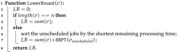The Lower Bound algorithm is shown in Algorithm 1.   

Algorithm 1: LowerBound

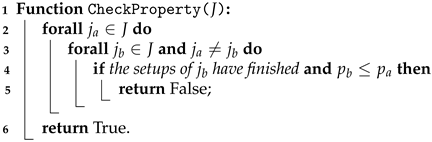
4.3. Dominance Property

In this section, after we use the lower bound to prune nodes, we also propose a property of the branch-and-bound algorithm (Algorithm 2), which can also speed up node pruning and reduce tree traversal time. The content description and proof of the property are as follows:

 Lemma 1.

Let $J=\{j_1,j_2,...,j_k\}$ be the unscheduled jobs at a node X in the branch-and-bound tree. For any unscheduled job $j_a$, if there is another unscheduled job $j_b$ such that the setups of $j_b$ are all scheduled and $p_b\le p_a$, then the subtree $X+j_a$ by choosing $j_a$ as the next job to schedule can be pruned off because $j_b$ precedes $j_a$ in some optimal solution.

Proof. 

Let $\sigma$ be the sequence of scheduled jobs. Assume that there is an optimal solution $(\sigma ,j_a,L,j_b)$, where L is a sequence of the unscheduled jobs. When the setups of job $j_a$ are not yet completed, its completion time $C_a$ would be $C_{\sigma }+{\sum }_{\begin{array}{c}i\to a\\ i\in unfinished\end{array}}^{m}s{p}_i+p_a$, and, when the setups of job $j_b$ are completed, its completion time $C_b$ would be $C_{\sigma }+C_a+C_L+p_b$, where $C_L$ is the completion time of all jobs of L. Assuming the positions of $j_b$ and $j_a$ are swapped as $(\sigma ,j_b,L,j_a)$, we denote their completion times as $C_b^{\prime }$,$C_L^{\prime }$, and $C_a^{\prime }$. At this point, $C_b^{\prime }$ will be $C_{\sigma }+p_b$, and $C_a^{\prime }$ will be $C_{\sigma }+C_b^{\prime }+C_L^{\prime }+{\sum }_{\begin{array}{c}i\to a\\ i\in unfinished\end{array}}^{m}s{p}_i+p_a$. Suppose that if $p_b$ is less than $p_a$, it makes $C_b^{\prime }$ less than $C_b$, which also makes the completion time of L shorter, to the benefit of both job $j_y$ and L. When both $C_y^{\prime }$ and $C_L^{\prime }$ move forward, the result of $C_a^{\prime }$ will also decrease accordingly. According to the assumption, we know that the total completion time of $(\sigma ,j_b,L,j_a)$ will be smaller than that of $(\sigma ,j_a,L,j_b)$. Therefore, we can prune off the branch of node $j_a$, which will not lead to a better solution without sacrificing the optimality.    □

Algorithm 2: Check Property

4.4. Tree Traversal

In this section, we use three different tree traversal methods, depth-first search (DFS), breadth-first search (BFS), and best-first search (BestFS), to perform the branch-and-bound algorithm. Moreover, we also added the upper bound, lower bound, and property mentioned above into our branch-and-bound algorithm.

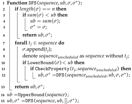
4.5. Depth-First Search (DFS)

DFS is a recursive algorithm for searching all the nodes of a tree and can generate the permutations of all the solutions. It starts at the root node and traverses along each branch before backtracking. The advantage of DFS is that the demand for memory is relatively low, but the disadvantage is that because of recursion, there will be a heavier loading in the stack operation, and it will take more time to find all the solutions. The DFS algorithm is shown in Algorithm 3.

First, the algorithm will obtain the upper bound from Line 15 and call the recursive DFS function. When we encounter the deepest node or have visited all of its children, we move backward along the current path to find the unvisited node to traverse. In the search process, we use LowerBound() and CheckProperty() to test whether we should continue to search down or not. If the lower bound is greater than or equal to the upper bound, or if the property is not met, we will prune the branch because it does not yield a better solution than the current one. This method can reduce the number of search nodes.   

Algorithm 3: Depth-First Search

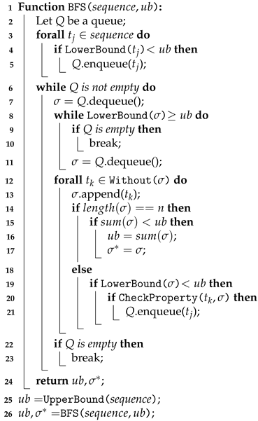
4.6. Breadth-First Search (BFS)

BFS is a tree traversal algorithm that satisfies given properties. It starts at the root of the tree, traverses all nodes at the current level, and moves to the next depth level. Unlike DFS, which will find a solution first, it will wait until the last level is searched to find all suitable solutions. In particular, this method uses a queue to record the sequence of visited nodes. The advantage of BFS is that each node is traversed by the shortest path, but the disadvantage is that it requires more memory to store all of the traversed nodes. It thus takes more time to search deeper trees.

The BFS algorithm is shown in Algorithm 4. First, the algorithm will obtain the upper bound by UpperBound() from Line 25. The BFS function starts from Line 2; we create a queue that uses the First-In-First-Out strategy. Lines 3 through 5 are the initial settings that we use to set a root. From Lines 6 to 24, we enqueue the root node and then dequeue the values in order. Then, we enqueue the unvisited nodes and recalculate the lower bound until there is no value in the queue. Before each enqueue, it is necessary to use LowerBound() and CheckProperty() to check whether the lower bound is smaller than the upper bound and whether it satisfies the property. It can reduce the number of visited nodes and shorten the execution time. In Line 12, we use the Without() function to obtain the nodes that have not been visited yet. The loop stops when the queue is empty, indicating that all nodes have been traversed.

Algorithm 4: Breadth-First Search

4.7. Best-First Search (BestFS)

BestFS works as a combination of depth-first and breadth-first search algorithms. It is different from other search algorithms that blindly traverse to the next node, it uses the concept of a priority queue and heuristic search, using an evaluation function to determine to which neighbor node is the best to move. It is also a greedy strategy because it always chooses the best path at the time, rather than BFS using an exhaustive search. The advantage of BestFS is that it is more efficient because it always searches through the node with the smaller lower bound first. On the other hand, the disadvantage is that the structure of the heap is difficult to maintain and requires more memory resources. Since each visited node will be stored in the heap, we can directly obtain the node with the smallest lower bound bound by heapsort. Therefore, when the amount of data is large, there will be too many nodes growing at one time, which will occupy a relatively large memory space.

The concept of the BestFS algorithm is the same as Algorithm 4. The difference is that in the BestFS function, we change the queue to a priority queue by using a min-heap data structure, where the priority order is sorted using the calculated lower bound, instead of using the FIFO order. The smaller the lower bound is, the higher the priority. When we use a heap to pop or push values, we will perform the function of heapify at the same time to ensure the heap is in the form of a min-heap. Heapify is the process of creating a heap data structure from a binary tree. Similarly, before each element is pushed into the heap, we use LowerBound() and CheckProperty() to check whether the lower bound is smaller than the upper bound and whether it satisfies the property.

5. Ant Colony Optimization (ACO)

Ant colony optimization (ACO) was proposed by Dorigo et al. [23] and Dorigo [24]. It is a meta-heuristic algorithm based on probabilistic techniques and populations. ACO is inspired by the foraging behavior of ants, where the probability of an ant choosing a path is proportional to the pheromone concentration on the path, that is, a large number of ant colonies will give positive feedback. When ants are looking for food, they constantly modify the original path through pheromones and, finally, find the best path. Initially, Ant System (AS) was used to solve the well-known traveling salesman problem (TSP). Later, many ACO variants were produced to solve different hard combinatorial optimization problems, such as assignment problems, scheduling problems, or vehicle routing problems. In recent years, some researchers have focused on applying the ACO algorithm to multi-objective problems and dynamic or stochastic problems. In ant colony optimization, each ant constructs its foraging path (solution) node by node. When determining the next node to move on, we can use dominance properties and exclusion information to rule out the nodes that are not promising. In comparison with other meta-heuristics, this feature may save the time required for handling infeasible or inferior solutions. The pseudo-code of ACO that we adopt is shown in Algorithm 5.

Algorithm 5: Ant Colony Optimization

State transition rule: We treat each job as a node in the graph and all nodes are connected. To choose the next edge, the ant will consider the visibility of each edge available from its current location, as well as the pheromones. The formula for calculating the visibility value is given by ${\eta }_{ij}=\frac{1}{{\displaystyle \sum _{i\to j}}s{p}_i+p_j}$, where ${\eta }_{ij}$ is the visibility value from node i to node j defined as the inverse of the processing time of job j plus its unfinished setup operations. Then, we will calculate the probability of each feasible path; the probability formula is given as $p_{ij}^k=\frac{{\tau }_{ij}^{\alpha }\ast {\eta }_{ij}^{\beta }}{{\displaystyle \sum _{k\in unselecte{d}_i}}{\tau }_{ik}^{\alpha }\ast {\eta }_{ik}^{\beta }},$ where ${\tau }_{ij}$ is the pheromone on the edge from node i to node j, $\alpha \ge 0$ is a parameter for controlling the influence of the pheromone, and $\beta \ge 0$ is a parameter for controlling the influence of invisibility. The next node is determined by a roulette wheel selection.

Pheromone update rule: When all ants have found their solutions, the pheromone trails are updated. The formula for updating the pheromones is defined as ${\tau }_{ij}=(1-\rho )\ast {\tau }_{ij}+△{\tau }_{ij}^k$, where $\rho$ is the pheromone evaporation rate, and $△{\tau }_{ij}^k$, the incremental of the pheromone from node i to node j by the kth ant, is ${\tau }_{ij}^k=\frac{Q}{\Sigma C_k}$ if the ant k traverses $edg{e}_{i,j}$; 0, otherwise, where $\Sigma C_k$ is the total completion time in the solution of the kth ant, and Q is a constant.

Stopping criterion: We set a time limit of 1800 s for the ACO execution. Once the course reaches the time limit, the ACO algorithm will stop and report the incumbent best solution.

To close the discussion of ACO features, we note that local search algorithms can improve on the ACO solution at each iteration and make the result closer to the global optimal solution. At the end of each ACO generation, we deploy a 2-OPT local search procedure to the best solution of each generation so as to probabilistically escape the incumbent solution away from the local optimum.

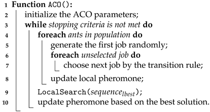6. Computational Experiments

In this section, we generate test data for appraising the proposed methods. The solution algorithms were coded in Python, and the integer programming models are implemented on Gurobi 9.1.2 interfaced with Python API. The experiments were performed on a desktop computer with Intel Core(TM) i7-8700K CPU at 3.70GHz with 32.0 GB RAM. The operating system is Microsoft Windows 10. We will describe the data generation design and parameter settings in detail and discuss the experimental results.

6.1. Data Generation Scheme

In the experiments, datasets were generated according to the following rules, and all parameters are integers:

• Six different numbers of jobs $n\in \{5,10,20,30,40,50\}$ and different numbers of setup operations $m\in \{4,8,18,25,35,45\}$.
• A binary support relation array $\mathcal{R}$ of a size $n\ast m$ is randomly generated. If $(s_i,t_j)$ belongs to $\mathcal{R}$, denoted by $r_{ij}=1$, then job $t_j$ cannot start unless setup $s_i$ is completed. The probability for $r_{ij}=1$ is set to be 0.5, i.e., if a generated random number $\le 0.5$, then $r_{ij}=1$. Note that when $r_{ij}=1$ for all i and j, the problem can be solved by simply arranging the job in the shortest processing time (SPT) order.
• The processing times of jobs $p_j$ were generated from the uniform distribution $[1,10]$.
• The processing times of setups $s{p}_i$ were generated from the uniform distribution $[1,5]$.
• For each job number, three independent instances were generated. In total, 18 datasets will be tested, as shown in

  Table 1. Categories of datasets.

  Datasets	n	m
  ${\mathcal{D}}_1,{\mathcal{D}}_2,{\mathcal{D}}_3$	5	4
  ${\mathcal{D}}_4,{\mathcal{D}}_5,{\mathcal{D}}_6$	10	8
  ${\mathcal{D}}_7,{\mathcal{D}}_8,{\mathcal{D}}_9$	20	18
  ${\mathcal{D}}_{10},{\mathcal{D}}_{11},{\mathcal{D}}_{12}$	30	25
  ${\mathcal{D}}_{13},{\mathcal{D}}_{14},{\mathcal{D}}_{15}$	40	35
  ${\mathcal{D}}_{16},{\mathcal{D}}_{17},{\mathcal{D}}_{18}$	50	45

  .

6.2. Results of Integer Programming Models

In the experiments of the integer programming models, we ran two integer programming models on the dataset with a time limit of 1800 s. The results are shown in

Table 2. Results of different IP models.

${\mathit{n}}_{\mathit{k}}$	Datasets	Position-Based			Sequence-Based			Best Solution
		obj.	Time	gap	obj.	Time	gap
5	${\mathcal{D}}_1$	101	0.09	0%	101	0.10	0%	101
	${\mathcal{D}}_2$	128	0.09	0%	128	0.10	0%	128
	${\mathcal{D}}_3$	122	0.08	0%	122	0.10	0%	122
10	${\mathcal{D}}_4$	461	246.11	0%	461	-	19%	461
	${\mathcal{D}}_5$	423	46.10	0%	423	-	21%	423
	${\mathcal{D}}_6$	457	355.95	0%	457	-	25%	457
20	${\mathcal{D}}_7$	2055	-	44%	2052	-	53%	2052
	${\mathcal{D}}_8$	1822	-	34%	1820	-	58%	1820
	${\mathcal{D}}_9$	1670	-	46%	1662	-	57%	1662
30	${\mathcal{D}}_{10}$	3609	-	50%	3602	-	61%	3597
	${\mathcal{D}}_{11}$	3985	-	50%	4007	-	62%	3985
	${\mathcal{D}}_{12}$	4448	-	62%	4469	-	66%	4424
40	${\mathcal{D}}_{13}$	8196	-	72%	8168	-	66%	8168
	${\mathcal{D}}_{14}$	7395	-	68%	7402	-	67%	7390
	${\mathcal{D}}_{15}$	7975	-	70%	7935	-	66%	7935
50	${\mathcal{D}}_{16}$	12,882	-	76%	12,963	-	66%	12,880
	${\mathcal{D}}_{17}$	12,305	-	73%	12,374	-	67%	12,305
	${\mathcal{D}}_{18}$	10,891	-	72%	10,953	-	66%	10,871

. If an IP model did not complete its execution of a dataset in 1800 s, its run time is denoted as ”−”. In the table, the $gap$ column indicates the relative difference between the feasible solution found upon termination and the best proven lower bound. The gap values were in the output of Gurobi. The gap value is defined as: $gap(\%)=\frac{|ObjBound-ObjVal|}{\left|ObjVal\right|}\times 100\%,$ where $ObjBound$ and $ObjVal$ are a lower bound and the incumbent solution objective, respectively. When the gap is zero we have demonstrated optimality. The column $bestsolution$ represents the best result of all our proposed methods on the same dataset.

When $n_k$ is 10, the sequence-based IP takes more than 1800 s, even though both methods can obtain the optimal solution. The position-based IP takes less time and ends up with a gap of $0\%$. When $n_k$ is greater than or equal to 20, neither model can find the optimal solution within 1800 s, but there are still some solutions that can find the same solution as the best solution, such as ${\mathcal{D}}_{17}$ of the position-based IP and ${\mathcal{D}}_{13}$ of the sequence-based IP. As $n_k$ increases, the gap of the position-based IP will be greater than that of the sequence-based IP. However, when we compare it with the best solution, even if the objective value is the same as the best solution, the gap value is still very large, such as the position-based IP of ${\mathcal{D}}_{17}$ and the sequence-based IP of ${\mathcal{D}}_7$ to ${\mathcal{D}}_9$. It means that their lower bounds are not tight, i.e., they have a significant deviation from the final feasible solution.

6.3. Results of Branch-and-Bound Algorithm

Table 3. Results of different tree traversal methods.

${\mathit{n}}_{\mathit{k}}$	Datasets	DFS				BFS				BestFS
		obj.	node_cnt	Time	dev	obj.	node_cnt	Time	dev	obj.	node_cnt	Time	dev
5	${\mathcal{D}}_1$	101	25	0.00	0.00	101	67	0.00	0.00	101	16	0.00	0.00
	${\mathcal{D}}_2$	128	22	0.00	0.00	128	44	0.00	0.00	128	12	0.00	0.00
	${\mathcal{D}}_3$	122	27	0.00	0.00	122	68	0.01	0.00	122	20	0.00	0.00
10	${\mathcal{D}}_4$	461	203	0.06	0.00	461	4141	0.39	0.00	461	283	0.04	0.00
	${\mathcal{D}}_5$	423	246	0.04	0.00	423	2518	0.27	0.00	423	128	0.02	0.00
	${\mathcal{D}}_6$	457	1055	0.25	0.00	457	34,646	2.57	0.00	457	1788	0.18	0.00
20	${\mathcal{D}}_7$	2052	34,798	69.07	0.00	7839	1,940,323	-	2.82	2052	33,393	22.62	0.00
	${\mathcal{D}}_8$	1820	44,844	77.49	0.00	6651	2,081,103	-	2.65	1820	44,166	22.03	0.00
	${\mathcal{D}}_9$	1662	201,418	314.67	0.00	6211	2,078,269	-	2.74	1662	172,094	96.32	0.00
30	${\mathcal{D}}_{10}$	3605	440,015	-	0.00	18,533	1,482,922	-	4.15	18,533	1,903,404	-	4.15
	${\mathcal{D}}_{11}$	4053	385,433	-	0.02	22,005	1,083,532	-	4.52	22,055	1,064,974	-	4.53
	${\mathcal{D}}_{12}$	4470	392,869	-	0.01	22,990	1,165,534	-	4.20	22,990	1,423,640	-	4.20
40	${\mathcal{D}}_{13}$	8357	189,796	-	0.02	51,610	846,721	-	5.32	51,610	769,918	-	5.32
	${\mathcal{D}}_{14}$	7564	176,723	-	0.02	44,779	873,638	-	5.06	44,779	1,112,645	-	5.06
	${\mathcal{D}}_{15}$	8074	185,522	-	0.02	49,102	888,079	-	5.19	49,102	1,094,652	-	5.19
50	${\mathcal{D}}_{16}$	13,007	74,873	-	0.01	106,541	856,905	-	7.27	106,541	954,605	-	7.27
	${\mathcal{D}}_{17}$	12,527	84,980	-	0.02	97,383	933,536	-	6.91	97,383	1,047,559	-	6.91
	${\mathcal{D}}_{18}$	11,255	90,908	-	0.04	87,545	1,055,329	-	7.05	87,545	1,181,533	-	7.05

shows the results of the branch-and-bound algorithm with three different tree traversal methods. We set the time limit to 1800 s. In this table, the column $node\_cnt$ represents the number of visited nodes. The $dev$ column is an abbreviation for deviation, expressed as a percentage of the difference between the objective value and the best solution. The calculation formula is as $dev(\%)=\frac{(obj-bestsolution)}{bestsolution}\times 100\%$.

When $n_k$ is less than 20, DFS and BestFS successfully find the optimal solutions, but their execution times and the number of visited nodes of BFS are much larger than others. Even if $n_k$ is 20, BFS cannot find the optimal solution within the time limit. In addition, we can see that the execution time of BestFS is faster than that of DFS for a small number of jobs. When $n_k$ is greater than or equal to 30, the three methods fail to find the optimal solution within the time limit. The number of visited nodes and the deviation of DFS are clearly lower than those of BFS and BestFS. The results indicate that DFS is more efficient than BFS and BestFS because the DFS algorithm is not a layer-order traversal but will backtrack after finding the solution. Therefore, BFS and BestFS may not be able to find any feasible solution within the time limit. To sum up, the performance of DFS is better than those of BFS and BestFS, so we will analyze the experimental results of DFS in detail in the next section.

6.4. Results of DFS Algorithm

In the experiment, we compare three different cases, including the original DFS algorithm, DFS with the lower bound, and DFS with the dominance property.

Table 4. Results of DFS algorithm.

${\mathit{n}}_{\mathit{k}}$	Datasets	DFS				DFS + LB				DFS + LB + Property
		obj.	node_cnt	Time	dev	obj.	node_cnt	Time	dev	obj.	node_cnt	Time	dev
5	${\mathcal{D}}_1$	101	325	0.00	0.00	101	28	0.00	0.00	101	25	0.00	0.00
	${\mathcal{D}}_2$	128	325	0.00	0.00	128	48	0.00	0.00	128	22	0.00	0.00
	${\mathcal{D}}_3$	122	325	0.00	0.00	122	27	0.00	0.00	122	27	0.00	0.00
10	${\mathcal{D}}_4$	461	9,864,100	173.53	0.00	461	614	0.11	0.00	461	203	0.07	0.00
	${\mathcal{D}}_5$	423	9,864,100	174.60	0.00	423	626	0.09	0.00	423	246	0.05	0.00
	${\mathcal{D}}_6$	457	9,864,100	182.09	0.00	457	2381	0.51	0.00	457	1055	0.25	0.00
20	${\mathcal{D}}_7$	2174	27,177,572	-	0.06	2052	135,187	230.35	0.00	2052	34,798	69.07	0.00
	${\mathcal{D}}_8$	2145	28,810,807	-	0.18	1820	287,087	429.71	0.00	1820	44,844	77.49	0.00
	${\mathcal{D}}_9$	1904	29,472,356	-	0.15	1662	1,006,390	1405.52	0.00	1662	201,418	314.67	0.00
30	${\mathcal{D}}_{10}$	4229	14,013,551	-	0.18	3679	426,340	-	0.02	3605	440,015	-	0.00
	${\mathcal{D}}_{11}$	4757	13,668,237	-	0.19	4211	462,562	-	0.06	4053	385,433	-	0.02
	${\mathcal{D}}_{12}$	5087	14,077,620	-	0.15	4530	443,418	-	0.02	4470	392,869	-	0.01
40	${\mathcal{D}}_{13}$	9557	7,184,349	-	0.17	8405	169,550	-	0.03	8357	189,796	-	0.02
	${\mathcal{D}}_{14}$	8505	7,327,087	-	0.15	7645	210,938	-	0.03	7564	176,723	-	0.02
	${\mathcal{D}}_{15}$	9131	7,111,936	-	0.15	8250	210,891	-	0.04	8074	185,522	-	0.02
50	${\mathcal{D}}_{16}$	14,629	4,136,372	-	0.14	13,196	104,445	-	0.02	13,007	74,873	-	0.01
	${\mathcal{D}}_{17}$	14,272	4,189,689	-	0.16	12,911	119,416	-	0.05	12,527	84,980	-	0.02
	${\mathcal{D}}_{18}$	12,901	4,254,099	-	0.19	11,522	114,774	-	0.06	11,255	90,908	-	0.04

shows the experimental results of the different cases and also compares their objective values $(obj.)$, numbers of visited nodes $(node\_cnt)$, execution times $\left(time\right)$, and deviations $\left(dev\right)$ from the best solution.

We can find that when the lower bound and properties are incorporated into DFS, the number of visited nodes is significantly reduced. Since this method will cut off unhelpful branches, it can also speed up the traversal, making it easier to find better solutions. Even when $n_k$ is greater than or equal to 30, none of the three cases can find the best solution within the time limit. However, compared with the original DFS, DFS with a lower bound and DFS with a dominance property attained smaller deviations, indicating the capability of finding solutions closer to the best solution.

6.5. Results of ACO Algorithm

In this section, we performed the ACO algorithm on the 18 datasets and set the time limit to 1800 s.

Table 5. Results of DFS with ACO upper bounds.

${\mathit{n}}_{\mathit{k}}$	Datasets	DFS			ACO		DFS + ACO
		obj.	node_cnt	Time	obj.	dev	obj.	node_cnt	Time
5	${\mathcal{D}}_1$	101	25	0.00	101	0.00	101	5	0.00
	${\mathcal{D}}_2$	128	22	0.00	128	0.00	128	7	0.00
	${\mathcal{D}}_3$	122	27	0.00	122	0.00	122	4	0.00
10	${\mathcal{D}}_4$	461	203	0.06	461	0.00	461	112	0.06
	${\mathcal{D}}_5$	423	246	0.04	427	0.01	423	75	0.04
	${\mathcal{D}}_6$	457	1055	0.25	464	0.02	457	954	0.25
20	${\mathcal{D}}_7$	2052	34,798	69.07	2058	0.00	2052	32,861	64.83
	${\mathcal{D}}_8$	1820	44,844	77.49	1868	0.03	1820	43,257	72.69
	${\mathcal{D}}_9$	1662	201,418	314.67	1668	0.00	1662	157,071	243.59
30	${\mathcal{D}}_{10}$	3605	440,015	-	3616	0.01	3597	433,789	-
	${\mathcal{D}}_{11}$	4053	385,433	-	3986	0.00	3985	373,573	-
	${\mathcal{D}}_{12}$	4470	392,869	-	4424	0.00	4424	357,690	-
40	${\mathcal{D}}_{13}$	8357	189,796	-	8282	0.01	8282	159,727	-
	${\mathcal{D}}_{14}$	7564	176,723	-	7390	0.00	7390	131,500	-
	${\mathcal{D}}_{15}$	8074	185,522	-	7967	0.00	7967	145,476	-
50	${\mathcal{D}}_{16}$	13,007	74873	-	12,880	0.00	12,880	69,077	-
	${\mathcal{D}}_{17}$	12,527	84,980	-	12,587	0.02	12,527	83,440	-
	${\mathcal{D}}_{18}$	11,255	90,908	-	10,871	0.00	10,871	71,311	-

,

Table 6. Results of BFS with ACO upper bounds.

${\mathit{n}}_{\mathit{k}}$	Datasets	BFS			ACO		BFS + ACO
		obj.	node_cnt	Time	obj.	Deviation	obj.	node_cnt	Time
5	${\mathcal{D}}_1$	101	67	0.00	101	0.00	101	4	0.00
	${\mathcal{D}}_2$	128	44	0.00	128	0.00	128	3	0.00
	${\mathcal{D}}_3$	122	68	0.01	122	0.00	122	4	0.00
10	${\mathcal{D}}_4$	461	4141	0.39	461	0.00	461	96	0.04
	${\mathcal{D}}_5$	423	2518	0.27	427	0.01	423	118	0.03
	${\mathcal{D}}_6$	457	34,646	2.57	464	0.02	457	2578	0.40
20	${\mathcal{D}}_7$	7839	1,940,323	-	2058	0.00	2052	43,231	33.67
	${\mathcal{D}}_8$	6651	2,081,103	-	1868	0.03	1868	3,185,673	-
	${\mathcal{D}}_9$	6211	2,078,269	-	1668	0.00	1662	79,117	124.83
30	${\mathcal{D}}_{10}$	18,533	1,482,922	-	3616	0.01	3616	782,158	-
	${\mathcal{D}}_{11}$	22,005	1,083,532	-	3986	0.00	3986	394,009	-
	${\mathcal{D}}_{12}$	22,990	1,165,534	-	4424	0.00	4424	485,726	-
40	${\mathcal{D}}_{13}$	51,610	846,721	-	8282	0.01	8282	649,800	-
	${\mathcal{D}}_{14}$	44,779	873,638	-	7390	0.00	7390	532,584	-
	${\mathcal{D}}_{15}$	49,102	888,079	-	7967	0.00	7967	702,847	-
50	${\mathcal{D}}_{16}$	106,541	856,905	-	12,880	0.00	12,880	682,047	-
	${\mathcal{D}}_{17}$	97,383	933,536	-	12,587	0.02	12,587	927,886	-
	${\mathcal{D}}_{18}$	87,545	1,055,329	-	10,871	0.00	10,871	820,528	-

and

Table 7. Results of BestFS with ACO upper bounds.

${\mathit{n}}_{\mathit{k}}$	Datasets	BestFS			ACO		BestFS + ACO
		obj.	node_cnt	Time	obj.	Deviation	obj.	node_cnt	Time
5	${\mathcal{D}}_1$	101	16	0.00	101	0.00	101	4	0.00
	${\mathcal{D}}_2$	128	12	0.00	128	0.00	128	3	0.00
	${\mathcal{D}}_3$	122	20	0.00	122	0.00	122	4	0.00
10	${\mathcal{D}}_4$	461	283	0.04	461	0.00	461	96	0.04
	${\mathcal{D}}_5$	423	128	0.02	427	0.01	423	61	0.02
	${\mathcal{D}}_6$	457	1788	0.18	464	0.02	457	1333	0.18
20	${\mathcal{D}}_7$	2052	33,393	22.62	2058	0.00	2052	13,380	24.48
	${\mathcal{D}}_8$	1820	44,166	22.03	1868	0.03	1820	39,031	25.69
	${\mathcal{D}}_9$	1662	172,094	96.32	1668	0.00	1662	71,082	100.10
30	${\mathcal{D}}_{10}$	18,533	1,903,404	-	3616	0.01	3616	1,350,098	-
	${\mathcal{D}}_{11}$	22,055	1,064,974	-	3986	0.00	3986	518,619	-
	${\mathcal{D}}_{12}$	22,990	1,423,640	-	4424	0.00	4424	648,245	-
40	${\mathcal{D}}_{13}$	51,610	769,918	-	8282	0.01	8282	790,216	-
	${\mathcal{D}}_{14}$	44,779	1,112,645	-	7390	0.00	7390	971,168	-
	${\mathcal{D}}_{15}$	49,102	1,094,652	-	7967	0.00	7967	1,087,057	-
50	${\mathcal{D}}_{16}$	106,541	954,605	-	12,880	0.00	12,880	888,985	-
	${\mathcal{D}}_{17}$	97,383	1,047,559	-	12,587	0.02	12,587	1,078,245	-
	${\mathcal{D}}_{18}$	87,545	1,181,533	-	10,871	0.00	10,871	1,181,376	-

summarize the results of the three branch-and-bound algorithms with ACO upper bounds. The results include objective values $(obj.)$ and deviation $\left(dev\right)$ of the ACO. The execution time of the ACO algorithm is much shorter than that of the branch-and-bound algorithm. In addition, we will compare the objective value $(obj.)$, the number of visited nodes $(node\_cnt)$, and the execution times, $\left(time\right)$, of the original algorithm and the algorithm with ACO as the upper bound. The ACO parameters used in the experiments are shown as follows: $generation=300$; $population=20$; $\alpha =3$; $\beta =1$; and $\rho =0.1$.

As can be seen from the experimental table, the deviation of the ACO is small and an even better solution can be found than IP models within 1800 s. Therefore, we can use the ACO as the initial value of the upper bound $\left(ub\right)$ to speed up the tree traversal time.

When the branch-and-bound algorithm is executing with the test $lb<ub$, the ACO can make $ub$ smaller, cutting more unnecessary branches. According to the tables, when $n_k$ is less than or equal to 20, the algorithm with an upper bound finds the best solution in a shorter time and visits fewer nodes; especially for the ACO in BFS, this is more obvious. As the value of $n_k$ becomes larger, it increases the probability of the algorithm finding the best solution within the same time limit. In summary, using the ACO solution as an upper bound can make the branch-and-bound algorithm perform better.

To summarize the computational study, we note that the two proposed integer programming approaches and the branch-and-bound algorithm, aimed at solving the problem to optimality, can complete their execution courses for 20 jobs or less. For larger instances, these exact two approaches become inferior. When reaching the specified time limit, the reported solutions are not favorable. Another observation is about the three traversal strategies. DFS has its advantages in its easy implementations (by straightforward recursions) and minimum memory requirement. The BFS and BestFS strategies are known to show their significance in maintaining acquired information about the quality of the unexplored nodes in a priority queue. On the other hand, they suffer from the memory space and heap manipulation work for the unexplored nodes. BFS and BestFS would be preferred when a larger memory is available and advanced data structure manipulations are available.

7. Conclusions and Future Works

In this paper, we studied the scheduling problem with shared common setups of the minimum total completion time. We proposed two integer programming models and the branch-and-bound algorithm, which incorporates three tree traversal strategies and the initial solutions yielded from an ACO algorithm. A computational study shows that the position-based IP outperforms the sequence-based one when the problem size is smaller. As the problem grows larger, the gap values for the sequence-based IP are smaller than those of the position-based IP. Similar to the branch-and-bound algorithm, the DFS performs best, regardless of whether lower bounds and other properties are used or not. Finally, we also observed that using ACO to provide an initial upper bound indeed speeds up the execution course of the branch-and-bound algorithm.

For future research, developing tighter lower bounds and upper bounds could lead to better performance. More properties can be found to help the branch-and-bound algorithm curtail non-promising branches. For integer programming models, tighter constraints can be proposed to reduce the execution time and optimality gaps to reflect a real-world circumstance in which multiple machines or servers are available for a software test project. In this generalized scenario, a setup could be performed on several machines if the jobs that it supports are assigned to distinct machines.

References

- Leung, J.Y.T. Handbook of Scheduling: Algorithms, Models, and Performance Analysis; CRC Press: Boca Raton, FL, USA, 2004. [Google Scholar]
- Pinedo, M. Scheduling; Springer: Berlin/Heidelberg, Germany, 2016. [Google Scholar]
- Kononov, A.V.; Lin, B.M.T.; Fang, K.T. Single-machine scheduling with supporting tasks. Discret. Optim. 2015, 17, 69–79. [Google Scholar] [CrossRef]
- Graham, R.; Lawler, E.L.; Lenstra, J.K.; Kan, A.R. Optimization and approximation in deterministic sequencing and scheduling: A survey. Ann. Discret. Math. 1979, 5, 287–326. [Google Scholar]
- Brucker, P. Scheduling Algorithms; Springer: Berlin/Heidelberg, Germany, 2013. [Google Scholar]
- Baker, K.E. Single Machine Sequencing with Weighting Factors and Precedence Constraints. Unpublished papers. 1971. [Google Scholar]
- Adolphson, D.; Hu, T.C. Optimal linear ordering. Siam J. Appl. Math. 1973, 25, 403–423. [Google Scholar] [CrossRef]
- Lawler, E.L. Sequencing jobs to minimize total weighted completion time subject to precedence constraints. Ann. Discret. Math. 1978, 2, 75–90. [Google Scholar]
- Hassin, R.; Levin, A. An approximation algorithm for the minimum latency set cover problem. In Lecture Notes in Computer Science; Springer: Berlin/Heidelberg, Germany, 2005; Volume 3669, pp. 726–733. [Google Scholar]
- Shafransky, Y.M.; Strusevich, V.A. The open shop scheduling problem with a given sequence of jobs on one machine. Nav. Res. Logist. 1998, 41, 705–731. [Google Scholar] [CrossRef]
- Hwang, F.J.; Kovalyov, M.Y.; Lin, B.M.T. Scheduling for fabrication and assembly in a two-machine flowshop with a fixed job sequence. Ann. Oper. Res. 2014, 27, 263–279. [Google Scholar] [CrossRef]
- Cheng, T.C.E.; Kravchenko, S.A.; Lin, B.M.T. Server scheduling on parallel dedicated machines with fixed job sequences. Nav. Res. Logist. 2019, 66, 321–332. [Google Scholar] [CrossRef]
- Brucker, P.; Jurisch, B.; Sievers, B. A branch and bound algorithm for the job-shop scheduling problem. Discret. Appl. Math. 1994, 49, 107–127. [Google Scholar] [CrossRef]
- Hadjar, A.; Marcotte, O.; Soumis, F. A branch-and-cut algorithm for the multiple sepot Vehicle Scheduling Problem. Oper. Res. 2006, 54, 130–149. [Google Scholar] [CrossRef]
- Kunhare, N.; Tiwari, R.; Dhar, J. Particle swarm optimization and feature selection for intrusion detection system. Sādhanā 2020, 45, 109. [Google Scholar] [CrossRef]
- Kunhare, N.; Tiwari, R.; Dhar, J. Intrusion detection system using hybrid classifiers with meta-heuristic algorithms for the optimization and feature selection by genetic algorithms. Comput. Ind. Eng. 2022, 103, 108383. [Google Scholar] [CrossRef]
- Luo, L.; Zhang, Z.; Yin, Y. Simulated annealing and genetic algorithm based method for a bi-level seru loading problem with worker assignment in seru production systems. J. Ind. Manag. Optim. 2021, 17, 779–803. [Google Scholar] [CrossRef]
- Ansari, Z.N.; Daxini, S.D. A state-of-the-art review on meta-heuristics application in remanufacturing. Arch. Comput. Methods Eng. 2022, 29, 427–470. [Google Scholar] [CrossRef]
- Rachih, H.; Mhada, F.Z.; Chiheb, R. Meta-heuristics for reverse logistics: A literature review and perspectives. Comput. Ind. Eng. 2019, 127, 45–62. [Google Scholar] [CrossRef]
- Blum, C.; Sampels, M. An ant colony optimization algorithm for shop scheduling problems. J. Math. Model. Algorithms 2004, 3, 285–308. [Google Scholar] [CrossRef]
- Yang, J.; Shi, X.; Marchese, M.; Liang, Y. An ant colony optimization method for generalized TSP problem. Prog. Nat. Sci. 2008, 18, 1417–1422. [Google Scholar] [CrossRef]
- Xiang, W.; Yin, J.; Lim, G. An ant colony optimization approach for solving an operating room surgery scheduling problem. Comput. Ind. Eng. 2015, 85, 335–345. [Google Scholar] [CrossRef]
- Dorigo, M.; Maniezzo, V.; Colorni, A. Positive Feedback as a Search Strategy; Technical Report 91–016; Dipartimento di Elettronica, Politecnico di Milano: Milan, Italy, 1991. [Google Scholar]
- Dorigo, M. Optimization, Learning and Natural Algorithms. Ph.D. Thesis, Dipartimento di Elettronica, Politecnico di Milano, Milan, Italy, 1992. (In Italian). [Google Scholar]