Article

An Improved Deep-Learning-Based Financial Market Forecasting Model in the Digital Economy

1
School of Finance, Central University of Finance and Economics, 39, South College Road, Beijing 100081, China
2
Collaborative Innovation Center of Green Development in the Wuling Shan Region, Yangtze Normal University, Chongqing 408100, China
3
Chongqing Vocational College of Transportation Jiangjin, Chongqing 402200, China
4
Fudan Postdoctoral Fellowships in Applied Economic Studies, Fudan University, Shanghai 200433, China
5
Guangxi Beibu Gulf Bank Postdoctoral Innovation and Practice Base, Nanning 530028, China
6
International College, Krirk University, Bangkok 10220, Thailand
*
Author to whom correspondence should be addressed.
Mathematics 2023, 11(6), 1466; https://doi.org/10.3390/math11061466
Submission received: 10 February 2023 / Revised: 11 March 2023 / Accepted: 14 March 2023 / Published: 17 March 2023

Abstract

:
The high-complexity, high-reward, and high-risk characteristics of financial markets make them an important and interesting study area. Elliott’s wave theory describes the changing models of financial markets categorically in terms of wave models and is an advanced feature representation of financial time series. Meanwhile, deep learning is a breakthrough technique for nonlinear intelligent models, which aims to discover advanced feature representations of data and thus obtain the intrinsic laws underlying the data. This study proposes an innovative combination of these two concepts to create a deep learning + Elliott wave principle (DL-EWP) model. This model achieves the prediction of future market movements by extracting and classifying Elliott wave models from financial time series. The model’s effectiveness is empirically validated by running it on financial data from three major markets and comparing the results with those of the SAE, MLP, BP network, PCA-BP, and SVD-BP models. Interestingly, the DL-EWP model based on deep confidence networks outperforms other models in terms of stability, convergence speed, and accuracy and has a higher forecasting performance. Thus, the DL-EWP model can improve the accuracy of financial forecasting models that incorporate Elliott’s wave theory.
MSC:
94-08; 94-04; 60G25; 68T07

1. Introduction

Financial markets are typically nonlinear and complex systems that are influenced by multiple, difficult-to-quantify factors. The purpose of industry and academic research on financial markets is to understand the laws of change, find reasonable and effective means to describe these laws in financial markets, and ultimately achieve predictions of future markets. Deep learning is the hottest technique in current neural network research and has been widely and successfully applied in many fields. Deep learning models use a multilayer network structure to learn feature information of the data layer by layer and autonomously abstract high-level feature representations from low-level features of the data. Arévalo et al. (2016) used deep learning to construct a high-frequency trading strategy [1]. Chong et al. (2017) used standard deep learning models to test three feature extraction techniques–principal component analysis (PCA), self-encoder, and restricted Boltzmann machine—and evaluated the feasibility of deep learning in predicting stock returns [2]. Fischer et al. (2017) applied the long short-term memory (LSTM) network for the prediction of the S&P 500 Index and compared LSTM with standard deep networks [3]. Wei et al. (2017) first applied stacked self-encoders for the prediction of the S&P 500 Index and compared them with standard deep neural networks (DNNs), logistic regression classifiers, and random forests, and were the first to apply stacked self-encoders to financial forecasting; their proposed deep learning model based on stacked self-encoders consisted of three parts: wavelet variation, stacked self-encoders, and LSTM. Interestingly, these outperformed other methods in terms of forecasting accuracy and profitability [4]. Basu, T. et al. (2022) utilized a Siamese-type neural network for pattern recognition in images followed by a bootstrapped image similarity distribution to predict rare events as they pertained to financial market analysis. The proposed method used a sliding window to store the input features as tabular data (HLC price), created an image of the time series window, and then used the feature vector of a pretrained convolutional neural network (CNN) to leverage pre-event images and predict rare events [5]. Navon and Kelly (2017) built an end-to-end deep learning model using raw financial time as input to successfully provide users with investment strategies [6]. SenGupta, I., Nganje et al. (2021) analyzed derivatives and commodity markets by using the improved Barndorff-Nielsen and Shephard (BN-S) model, which had the advantages of a high efficiency, few parameters, and completely random data extraction [7]. Troiano et al. (2017) used a restricted Boltzmann machine and a self-encoder to build two separate deep learning models to predict the future trend of the S&P Index; comparing the advantages and disadvantages of the two models, the authors found that the self-encoder performed better [8]. However, as they concluded, research in this area of deep learning for financial forecasting was still in its infancy and needed to be improved. Moreover, they argued that the number of input data and the type of indicators as well as the determination of the range of up or down of the output were open to question.
The Elliott wave can be considered as a high-level abstract representation of financial time series, and thus feature extraction is a key point in financial forecasting models [9]. The multilayer network structure of deep learning models can achieve this better. However, to the best of our knowledge, there is no published literature at the research stage on modeling Elliott wave models using deep learning techniques. The literature typically uses volume as input data (Volna et al., 2013) [10]. This is contrary to the Elliott Wave Theory, which takes the highest and lowest prices of stock prices as the object of study and volume is only an auxiliary indicator. Some studies in this area include Zhen Wu et al.’s (2004), who applied the rules of Elliott’s wave theory to wavelet-packet-decomposition-extracted features from financial time series and then used a genetic neural network (GNN) to predict the short-term changes in stock prices [11]. Qingfeng Li et al. (2011) combined a Fourier transform and a BP neural network to analyze the stock spectrum and were able to fit the Elliott wave [12]. Fuzzy neural networks have also been successfully combined with Elliott’s wave theory for predicting future market movements (Elaal et al., 2012) [13]. Atsalakis et al. (2012) [14] combined Elliott’s wave theory to build a neurofuzzy system called wave analysis stock prediction (WASP) for stock market prediction. This method used the mean and oscillator as key reference tools for analyzing the Elliott Wave. However, the mean and oscillator were only artificially set by the trading software program to help the participants analyze the market. The settings of their model had limitations that could affect the accuracy of the model prediction.
A major innovation of this study is attempting to model financial time series using deep learning models. To the best of our knowledge, we propose the first deep learning + Elliott wave principle (DL-EWP) model based on deep confidence networks for abstracting and identifying the Elliott wave models in financial time series. Using these extracted and classified Elliot wave models, we then empirically demonstrate the effectiveness of this model’s prediction of future market trends versus those by other models. Five reference models are used to model the Elliott wave model recognition in financial time series, and then we comprehensively compare the performance with various neural networks. The reference models include three deep learning models, and traditional BP networks and their improvement networks. The comparative analysis demonstrates that the DL-EWP model based on the deep confidence network outperforms other models in terms of stability, convergence speed, and accuracy and has higher prediction performance.
The remainder of this study is structured as follows: The second part reviews the related work on deep learning and wave theory. We describe the association between wave theory and deep learning, and the theoretical basis for building a deep learning model to solve our specified problem. The third part outlines the principles of building deep learning models integrating the Elliot Wave Theory. Specifically, we clearly describe the principles and construction process of the DL-EWP model as well as reference models, with the structure of the DL-EWP model based on the general framework of financial prediction models. In the fourth part, we empirically test the DL-EWP model. We first select the relevant categories of financial data and outline the basis of their selection. Then, we preprocess the original financial time series. Finally, we empirically demonstrate the validity of the model. The fifth part undertakes the comparison of the models. By introducing five reference models for modeling the Elliott wave model recognition of financial time series, the performance effectiveness of multiple neural network models is comprehensively compared and investigated. Finally, the seventh part presents the conclusions of this study.

2. Related Work

2.1. Deep Learning

Deep learning uses a multilayer network structure to learn the feature information of data layer by layer and autonomously abstracts high-level feature representations from the low-level data features. Deep learning effectively improves the problems such as local optimum and gradient disappearance of BP networks. Furthermore, it has a better representation capability than shallow networks and is thus more suitable for modeling Elliott wave models.

2.1.1. Deep Belief Network

Deep belief network (DBN) is a classical model of deep learning. It is a deep generative network made by stacking multiple stack units. A multilayer restricted Boltzmann machine (RBM) and a BP classifier are the classical architecture of DBNs, as shown in Figure 1. DBNs combine unsupervised learning (RBMs) and supervised learning (BP) [15].

2.1.2. Training of Deep Confidence Networks

Training a DBN consists of two phases: pretraining and fine-tuning (Hinton et al., 2006). The pretraining phase adopts an unsupervised greedy layer-by-layer learning strategy to train each constrained Boltzmann machine layer by layer from the bottom up. This process enables the layer-by-layer extraction of feature information from the original data and in turn, abstracts the high-level feature representation of the data. The fine-tuning phase uses supervised learning algorithms (e.g., BP algorithms and support vector machines) to tune some or all of the parameters of the network, through which the task of classification and recognition can be accomplished. The BP network used for the classification task in the fine-tuning phase is generally located at the last layer of the DBN [16].
The pretraining phase is the process of training multiple RBMs from the bottom up. An RBM model is determined by the parameters θ = { w , c , b } , where w denotes the weight between the visible and hidden layer units, and b and c denote the offsets of the visible and hidden layer units, respectively. The output value obtained from each RBM layer is used as the input of the next RBM layer, and the feature vector set of samples is obtained layer by layer. The pretraining process is to adjust the parameters of the RBM model for each layer, which only guarantees the optimal output result of this layer but not of the whole DBN. Therefore, a backpropagation process is needed to tune the DBN parameters. The fine-tuning process is top-down, using the sample data label set Y and the BP algorithm to adjust the network parameters θ = { w , c , b }  [17].
For a DBN with l hidden layers, the joint probability distribution is expressed as follows.
P ( v , h 1 , h 2 , , h l ) = p ( v | h 1 ) p ( h 1 | h 2 ) p ( h l 2 | h l 1 ) p ( h l 1 , h l )
Equation (1) reflects the feature that the DBN is superimposed by RBMs, which is the probability distribution of the RBM at the top level, and p ( h k | h k + 1 ) is the conditional probability training ( k = 0 , 1 , 2 , , l 1 , among them h 0 = v ) of hidden layer h k of the RBM at each layer under the h k + 1 state of known visible layers. The classification problem can be solved using a DBN.
The training sample set is:
X = ( x 0 , x 1 , x n )
The data label set is:
Y = ( y 0 , y 1 , , y n )

2.2. Elliott Wave Theory

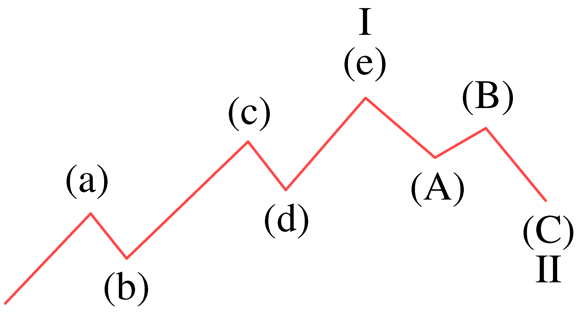
The American scholar R.N. Elliott discovered and proposed a wave theory after a long-term study of the Dow Jones Industrial Average. Elliott’s wave theory describes the occurrence and development of phenomena in nature in terms of cyclic waves. A complete cyclic wave consists of a driving wave and an adjustment wave. The term “drive” refers to the behavior of the market in the direction of the trend, and “adjustment” refers to the behavior of the change in the opposite direction of the trend. In financial markets, the adjustment wave completes a partial price retracement of the driving wave, and this retracement behavior follows the golden ratio relationship. Usually, the driving wave has a five-wave structure (1-2-3-4-5) and the adjustment wave has a three-wave structure (a-b-c). Depending on the direction of the trend, there are bull (trend direction up) and bear markets (trend direction down) in financial markets. When the main trend is up, a complete cyclic wave is shown in Figure 2 [18].
In the Elliott wave shown in Figure 2, wave I is the driving wave, wave II is the adjusting wave of wave I, and waves I and II are composed of smaller versions of driving and adjusting waves. In wave I, waves (a), (b), and (c) are driving waves, while waves (b) and (d) are the adjusting waves of waves (a) and (c), respectively. In wave II, waves (A) and (C) are driving waves, and wave (B) is an adjusting wave. By analogy, waves (a)–(e) and (A)–(C) are composed of smaller driving and adjusting waves. That is, they both consist of the driving wave of a five-wave structure and the adjusting wave of a three-wave structure. Waves I and II in Figure 2 are defined as “cyclical waves”, and waves (a)–(e) and (A)–(C) are defined as “large waves” (Frost and Prechter, 1998). Importantly, the fractal level of a “cyclic wave” is one level smaller than that of a “large wave”. Waves (1)–(5) and (A)–(C) in Figure 2 are called “medium waves”, and their fractal level is one level smaller than that of “large waves”. As long as the trading behavior of the financial markets does not stop, the fractal level of waves will continue to increase over time; this development is in line with the law of logarithmic spiral change.
A complete cyclic wave consists of a driving wave and an adjustment wave. The driving wave consists of five waves, and the adjusting wave consists of three waves or their variants. The “adjustment” is a partial retracement of the “driving” price, and the relationship of this partial retracement satisfies the golden mean. The Fibonacci series is the linear recursive series 1, 1, 2, 3, 5, 8, 13, 21, 34, 55, , and the series is defined by the following equation:
F ( n ) = 0 n = 0 1 n = 1 F ( n 1 ) + F ( n 2 ) n > 1
Elliott’s wave theory embodies the characteristics of the Fibonacci series in many ways, most notably in the relationship between the number of waves and the price ratio. The number of Elliott’s waves belongs to the Fibonacci series, and the price of the adjustment wave is usually 0.618 or 0.382 in relation to the previous driving wave.
When applying wave theory to forecast the future trend of financial markets, correctly determining the current Elliott wave model in which the market is located is a key point in solving the problem. For example, when the market completes a complete upward five-wave structure, it will face a three-wave downward adjustment; when the market ends a three-wave structure adjustment, it will face a five-wave bull market. The main purpose of the forecasting model is to accurately identify the model of Elliott waves from the financial time series.

3. Constructing a Model Integrating Deep Learning and Elliott Wave Theory

Elliott’s wave theory reveals the fundamental laws of financial market fluctuations and is an important tool for financial analysis. If an effective method can be found to extract Elliott wave models from financial data, it will be a big breakthrough for financial forecasting. Inspired by this, this study sought to model Elliott waves using the deep learning model of a DBN network, with each RBM layer extracting features from input data by energy function and finally classifying the model of waves using the BP network layer. The basic trading data of financial market include the opening price, volume, closing price, etc. The Elliott wave is a price sequence consisting of the highest or lowest price.
The advantage of deep learning lies in the ability to achieve feature information extraction of data layer by layer using a multilayer network structure, and deep learning is successfully applied in many fields, but no published research on using deep learning techniques for Elliott wave pattern modeling was found in the research phase, and this paper innovatively proposes a DBN-based EWP deep learning model (PLR_VIP + DBN), which consists of two main parts. The first part is a segmented linear representation based on significant points (PLR_VIP algorithm), which achieves the role of normalizing the step size of financial time series while preserving the significant feature points of the original financial time series; the second part is a deep confidence network, and the DBN network finally obtains the Elliott wave pattern corresponding to the series through feature extraction and the classification of the financial time series, so as to predict the future financial market. The effectiveness of the EWP model is verified through experiments.
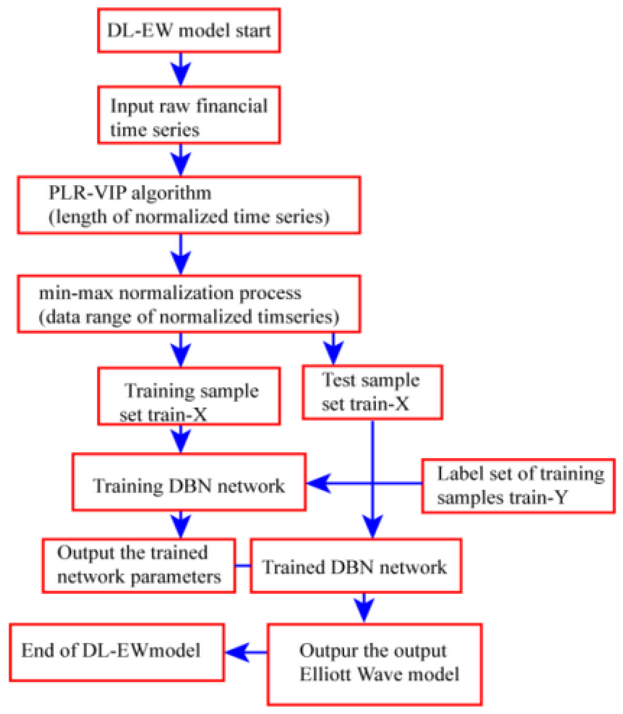
Our DL-EWP model consists of three main components: the segmented linear representation algorithm based on significant points, a min-max normalization, and the DBN network. Using this model, we can identify Elliott wave models in financial time series. The training and testing of the DBN network are two important steps in the construction of the DL-EWP model. The training phase results in a suitable configuration of the network parameters so that the trained network can be used to predict the Elliott wave models of the financial time series. Both the training and test sample sets are obtained from the original financial time series using a segmented linear representation algorithm based on significant points and a min-max normalization method. Figure 3 shows the basic framework of the DL-EWP model.
On the one hand, the time to complete an Elliott wave at different stages of the financial market is often not deterministic, i.e., the step size of the original financial time series is nonstandard. On the other hand, the number of input neurons of the DBN network needs to be specified. The segmented linear representation algorithm based on significant points can standardize the step length of financial time series while preserving the significant points of the original series. The range of price fluctuations varies widely among different financial time series, and the accuracy and convergence speed of the network are affected when the DBN network is trained directly using these data. Then, the min-max normalization method can standardize the range of the variation of the original financial time series, eliminate the influence of multiple orders of magnitude on the network, and improve the network’s accuracy and convergence speed [19]. This process is illustrated in Figure 4.
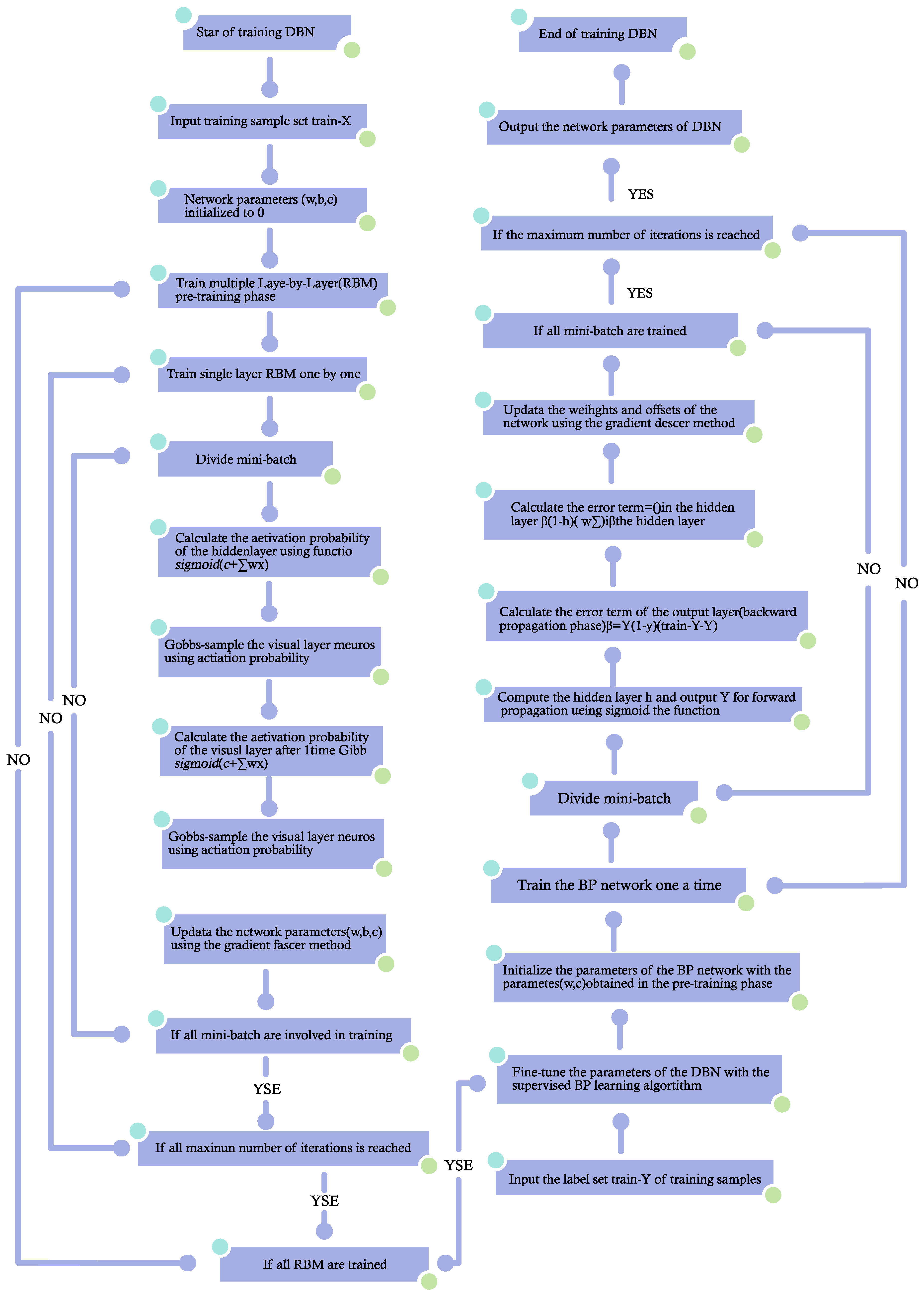
The parameters of the DBN network are directly related to the prediction results of the Elliott wave model recognition. Therefore, training the DBN network with a preprocessed sample dataset is a key step in building the DL-EWP model. Hence, the RBM is trained bottom-up using the training sample set, and the sigmoid function is used to calculate the activation probability of each neuron in each layer. Then, the Gibbs sampling of the visual layer neurons is performed using the activation probability and the parameters are finally updated using the gradient descent method. The RBM is trained iteratively until it reaches a preset number of iterations. Then, the label set of training samples is input, and the weights and offsets of the DBN network are iteratively adjusted using a supervised backpropagation learning algorithm to finally obtain a DBN network capable of successfully predicting the Elliott wave models of financial time series. The specific algorithmic flow of training the DBN network in the DL-EWP model is shown in Figure 5.

4. Empirical Validity of the DL-EWP Model

4.1. Data Selection

Trading price data were selected from the following three sources: global stock index, foreign exchange market, and commodities. The financial market is the place where commodity exchange is realized: commodities contain the basic materials for production and life; foreign exchange is the medium and contract for commodity exchange; and stock indices represent the overall economic situation of a country. Therefore, the trading data of these three major markets can comprehensively reflect the overall situation of financial markets. Elliott’s wave theory studies the inherent characteristics of the financial market and describes the basic trading data of the financial market, with each Elliott wave comprising the highest and lowest prices. Therefore, the data used here were the opening, closing, highest, and lowest prices of global stock, foreign exchange, and commodities markets. The details are shown in Table 1.
The DBN network consisted of multiple RBMs and a BP classifier. The parameter configuration of the DBN network was directly related to the prediction results of the Elliott wave pattern recognition; therefore, training the DBN network using the sample dataset obtained after preprocessing was a key step in building the EWP deep learning model. The DBN network parameters w, b, and c were initialized to zero, and the DBN network was trained layer by layer from the bottom up using the training sample set. The RBM was trained bottom-up using the training sample set, and the sigmoid function was used for each layer to calculate the activation probability of the neuron. The activation probability calculated by the sigmoid function was used to Gibbs sample the neurons in the visual layer, and finally the parameters were updated using the gradient descent method, while choosing the mean square error to measure the reconstruction error. The RBM was trained iteratively until a preset number of iterations was reached. Then, the label set of training samples was input, the weights and offsets of the DBN network were iteratively adjusted using a supervised backpropagation learning algorithm, and finally, a DBN network capable of successfully predicting Elliott wave patterns of financial time series was obtained. The specific algorithmic flow of training the DBN network in the EWP deep learning model is shown in Figure 5.
A total of 6092 Elliott wave samples were drawn from the historical price data of 18 traded instruments in the three types of markets. The sample of global stock indices, foreign exchange market, and commodities accounted for 26.7%, 30.7%, and 42.6% of the total sample, respectively. The basic information about the extracted data is listed in Table 2.

4.2. Data Preprocessing

The preprocessing stage consisted of two steps: the segmented linear representation algorithm and the min-max normalization process. The aim of preprocessing was to normalize the time series’ step size and data range.

4.2.1. Segmented Linear Representation Algorithm

The time required to complete an Elliott wave structure in financial markets is usually uncertain, and the lengths of financial time series constituting the same wave model may vary. Therefore, we needed to fix the step length of the original time series beforehand and thus determine the number of neurons in the input layer of the deep learning model. The purpose and method of this operation were equivalent to those of the time series representation in time series mining. This operation also enabled data compression and feature extraction. To ensure that the time series obtained after preprocessing contained the important inflection points that made up the Elliott wave, we preprocessed the original financial time series using a segmented linear representation algorithm based on important points. This algorithm was referred to as PLR_VIP, where PLR stands for piecewise linear representation, V stands for vertical distance, and IP stands for important point [20].
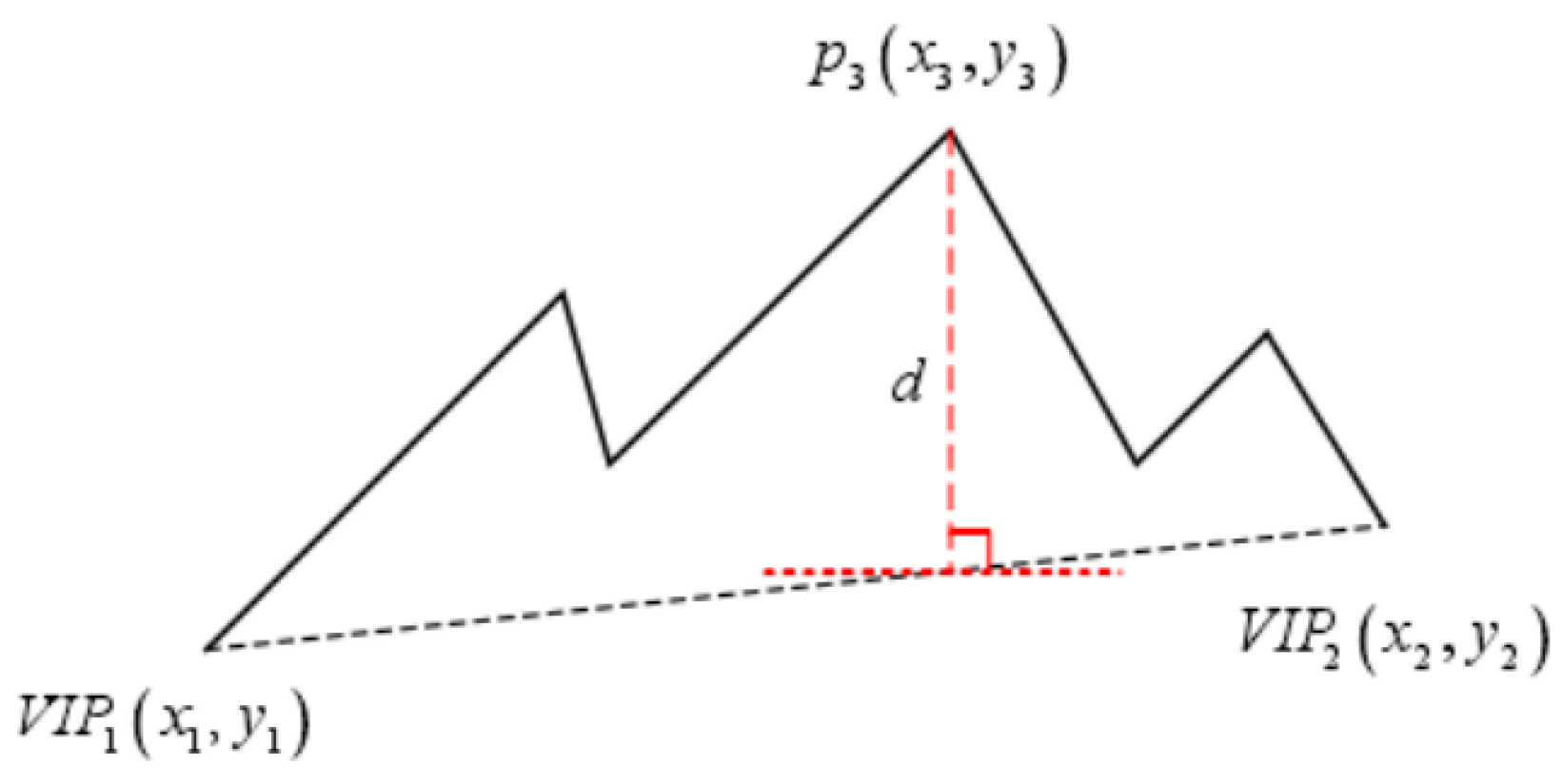
The basic idea of the PLR_VIP algorithm was as follows: First, the two endpoints VIP1 and VIP2 defaulted to important points. Then, the point p with the farthest vertical distance from the endpoint was found in the region and marked as the next important point VIP3. Subsequently, the points with the farthest vertical distance were found in the region with VIP1 and VIP3, and VIP3 and VIP2 as endpoints, and marked as important points, respectively. The above process was iterated until the set number of significant points was reached. Figure 6 shows the basic idea of the PLR_VIP algorithm, while Algorithm 1 shows the specific operation of the PLR_VIP algorithm [21].
Mathematics 11 01466 i001

4.2.2. Min-Max Normalization

The price data of financial transactions have a large range of variation. For example, the data on the S&P500’s price fluctuations used here were distributed in the range [ 0.4 , 3000 ] , while those for the Dow Jones Industrial Index were in the range [20, 27,000]. Moreover, there were large fluctuations in price changes within a single sample in the sample set of the Elliott wave model. During the training process of the network, data of larger order of magnitude could mask the effect of data of smaller order of magnitude on the network; in turn, this could affect the network’s accuracy. In addition, the data range was not uniform between samples, and the base and mean values varied widely. This increased the difficulty of network training and could lead to slow convergence. Therefore, we needed to normalize the sample data by using the min-max normalization method to map the sample data to the interval [ 0 , 1 ] . The min-max normalization of the i th data x i of sample yielded x i [22]:
x i = x i min ( x ) max ( x ) min ( x )

4.2.3. Example of Data Preprocessing

The results of the step normalization using the PLR_VIP algorithm for a wave sample of the S&P 500 Index are shown in Figure 7b. Notably, the PLR_VIP algorithm achieved the effect of normalizing the step size while preserving the main features (i.e., significant points) of the original time series.

4.3. Design of the Elliott Wave Model

The key to using Elliott’s wave theory to forecast financial markets is to accurately identify the current Elliott wave model in which the market is operating. When the current wave model is known, the future trend and structure of the market can be accurately predicted [23].
After studying and summarizing the Elliott wave theory, this study designed eight types of Elliott wave models consisting of eight subwaves, as shown in Figure 8.
A basic, complete Elliott wave is composed of eight subwaves. For regular driving and adjusting waves (i.e., except in the case of triangles), the most straightforward design idea is to aim at identifying the complete eight-wave structure, and thus target the beginning of bullish (models 1 and 2) and bearish (models 3 and 4) markets. Since regular adjustment waves are differentiated between saw-tooth (models 1 and 3) and platform (models 2 and 4), there is a distinction between two models for bull and bear markets. The structure of a correction wave is more complex than a driving wave and is typically longer as well. For example, the US Dollar Index has been in a corrective wave since 1985. This makes it difficult and necessary to accurately analyze the structure of a correction wave. In an adjustment wave, targeting the C wave and its third subwave (i.e., the main dip) is a key task. This study devised models 5 and 6 for predicting the main dip in a flat and saw-tooth adjustment wave, respectively. For unconventional driving and adjusting waves, such as triangle waves, our main objective was to predict the trend up (model 7) or down (model 8) without having to specifically distinguish between driving or adjusting. According to Elliott’s wave theory, the end of a triangle structure often means that the market will enter a “sprint” phase. Although triangles are less frequent, the identification of this structure is still highly relevant [24].

4.4. Design of DBN Network Parameters

Setting network parameters is crucial for the effectiveness of the prediction model. This process mainly includes the following aspects: the number of neurons in the output and input layers, the number of layers in the hidden layer and the number of neurons in each layer, the learning rate in the pretraining and fine-tuning stages, and the number of iterations of pretraining and fine-tuning. The PLR_VIP algorithm processing indicated that the length of the financial time series of each sample was 15. Thus, the number of neurons in the input layer of the DBN network was set to 15. As noted, there were eight types of Elliott wave models. Therefore, the output layer was set to eight neurons. The number of layers and neurons in the hidden layer affect the accuracy of the DBN network. Meanwhile, the learning rate, momentum factor, and the number of iterations are related to the convergence speed, error, and stability of the network. After several trial experiments, we settled on a DBN network with a two-layer RBM structure, and its specific parameters are listed in Table 3.
In the training process of the network, the momentum factor term α was added to the weight update process to weaken the oscillation phenomenon when the error changed.

4.5. Empirical Results of the DL-EWP Model

The original financial time series were normalized by the PLR_VIP algorithm and min-max normalization in the preprocessing stage to obtain the sample data for training and testing the DBN network. The DBN network was then trained iteratively using the training samples in two parts: pretraining and fine-tuning. After the pretraining, the reconstruction error of the two-layer RBM network was 2.626. In the fine-tuning phase, the mean square error (MSE) of the samples with the BP classifier for the classification task changed as the number of iterations increased, as shown in Figure 9.
The training tuned the DBN network parameters on the training sample set, and thus gave us a DL-EWP model capable of predicting the Elliott wave models of financial time series. The model was then used to classify 1164 financial time series for Elliott wave model prediction. The results showed that a total of 793 test samples were correctly classified. The accuracy of the DL-EWP prediction model was 68.13%, while its MSE was 0.4066. The experiments demonstrated that the proposed DL-EWP could effectively recognize Elliott wave models in financial time series.
Next, we present the forecasting results of the DL-EWP model for financial time series. Selected data for three major types of financial markets were drawn from the test sample, corresponding to the S&P 500 Index (global stock index), the Euro Index (foreign exchange market), and WTI crude oil (commodity). In the monthly S&P 500 price data in Figure 10a, the DL-EWP model accurately identified the financial time series between July 1933 and March 1937 as Elliott wave model 4, between March 1937 and October 1939 as model 6, and between April 1942 and June 1949 as model 1. In the quarterly Euro Index price data in Figure 10b, the DL-EWP model successfully identified the financial time series between June 1985 and December 2000 as model 2, and between December 2006 and June 2015 as model 7. In the monthly WTI crude oil price data in Figure 10b, the DL-EWP model successfully identified the financial time series between June 1985 and December 2000 as model 3, and between December 2006 and June 2015 as model 4. Finally, in the monthly WTI crude oil price data in Figure 10c, the DL-EWP model identified the financial time series between October 1990 and October 1997 as model 5, and between February 1999 and November 2001 as model 1.

5. Comparison of Models

In addition to DBN networks, five related neural network models were used to compare the performance of DL-EWP model: SAE (AEs + BP), MLP (BPs), BP network, PCA-BP, and SVD-BP models. The first two are deep learning models, while the last three are shallow network models with single-layer networks. We then empirically validated the effectiveness and superiority/inferiority of the DL-EWP model.

5.1. Selecting Evaluation Criteria

To evaluate the prediction performance of the deep learning models, four performance indicators were used: MSE, root-mean-square error (RMSE), mean absolute error (MAE), and error rate (ER). The calculation formulae for each are listed in Table 4.
Note: T i denotes the predicted true value, P i denotes the predicted value of the model, M o d e l p denotes the Elliott wave model predicted by the model, M o d e l r denotes the true Elliott wave model, and n denotes the sample size.
Lower values of these metrics indicate that the prediction results of the prediction model are closer to the true results. The notable metric is the ER, which is calculated as the ratio of the number of samples with wrongly predicted wave models to the number of all tested samples. We were most concerned about the ER because it is directly related to the accuracy of users’ trading decisions. Meanwhile, the ER also indirectly reflects the prediction model’s ability to extract features from the sample data.

5.2. Parameter Design of the Reference Model

The SAE model had two self-encoders, the MLP model had two hidden layers, and the BP network, PCA-BP, and SVD-BP models were shallow network models with a single hidden layer. Similar to the DL-EWP model, the reference models also included a preprocessing step to normalize the time series step and data range. The network parameters of the above five reference models are shown in Table 5, Table 6 and Table 7.
In the PCA-BP model, the PCA algorithm reduced the step size of the financial time series from 15 to 10. Therefore, the network input layer of the PCA-BP model had a total of 10 neurons.

5.3. Comparison of the DL-EWP Model’s Performance

We empirically checked the effectiveness of the six forecasting models: DL-EWP, SAE, MPL, BP network, PCA-BP, and SVD-BP models. Table 8 lists the performance of all models on the four evaluation metrics. Interestingly, all six forecasting models could successfully predict the Elliott wave model for the financial time series. However, the effectiveness of each model’s prediction performance differed. The DL-EWP model outperformed the other models, while the SVD-BP model showed a relatively poor prediction performance.
The prediction performance of the deep and shallow networks also differed. Among the shallow network models, the PCA-BP model had the lowest values of MSE, RMSE, and MAE, and the lowest ER value. By contrast, among the deep network models, the DL-EWP model had the lowest values of MSE, RMSE, MAE, and ER, and the best performance; it had 41.08%, 23.23%, and 38.67% lower MSE, RMSE, and MAE values, respectively, than those of the PCA-BP model. Furthermore, the ER value of the DL-EWP model was 36.69% lower compared to that of the BP network model. Together, the mean MSE, RMSE, MAE, and ER values for the three deep network models were 0.4974, 0.7107, 1.1161, and 37.74%, respectively, while those for the three shallow network models were 0.7656, 0.8740, 1.4582, and 61.65%, respectively. That is, the deep network model had 35.03%, 18.68%, 23.46%, and 38.78% lower values, respectively, than the shallow network models. This demonstrated the superiority of the deep learning model. This also indicated that deep networks could improve the problem of the weak characterization ability of shallow networks.
Next, the DL-EWP model was compared with each reference model. Among the three deep network models, the error rate of the DL-EWP model was 10.83% and 30.14% lower, and the accuracy was 6.02% and 25.29% higher than that of the SAE and MLP models, respectively. Among the three shallow network models, the BP network had the lowest error rate; however, the DL-EWP model had a 36.69% lower error rate and a 37.19% higher accuracy than the BP network. Thus, the DL-EWP model had the lowest prediction error rate, which indirectly demonstrated that the feature extraction ability of the DL-EWP model was higher than that of the reference models. The performance of the SAE model was second only to the DL-EWP model on all four evaluation criteria. Meanwhile, the performance of the SVD-BP model was worse than the other five models on all four evaluation criteria. In comparison, the DL-EWP model reported 52.97%, 31.42%, 43.70%, and 60.20% lower MSE, RMSE, MAE, and ER values, respectively. Thus, the DL-EWP model outperformed the SVD-BP shallow network model and was slightly better than the SAE deep learning model. Among the shallow network models, the training error of the PCA-BP model was smaller than that of the BP network, but its error rate was higher. Thus, the introduction of the PCA algorithm into the BP network resulted in overfitting, which was reflected by a weaker generalization ability of the traditional BP network for samples with larger quantities of data.
Together, these results showed that the prediction performance and feature extraction ability of the DL-EWP model were better than those of the reference models. Moreover, the prediction performance and feature extraction ability of the deep network models were higher than those of the shallow network models based on the BP network.
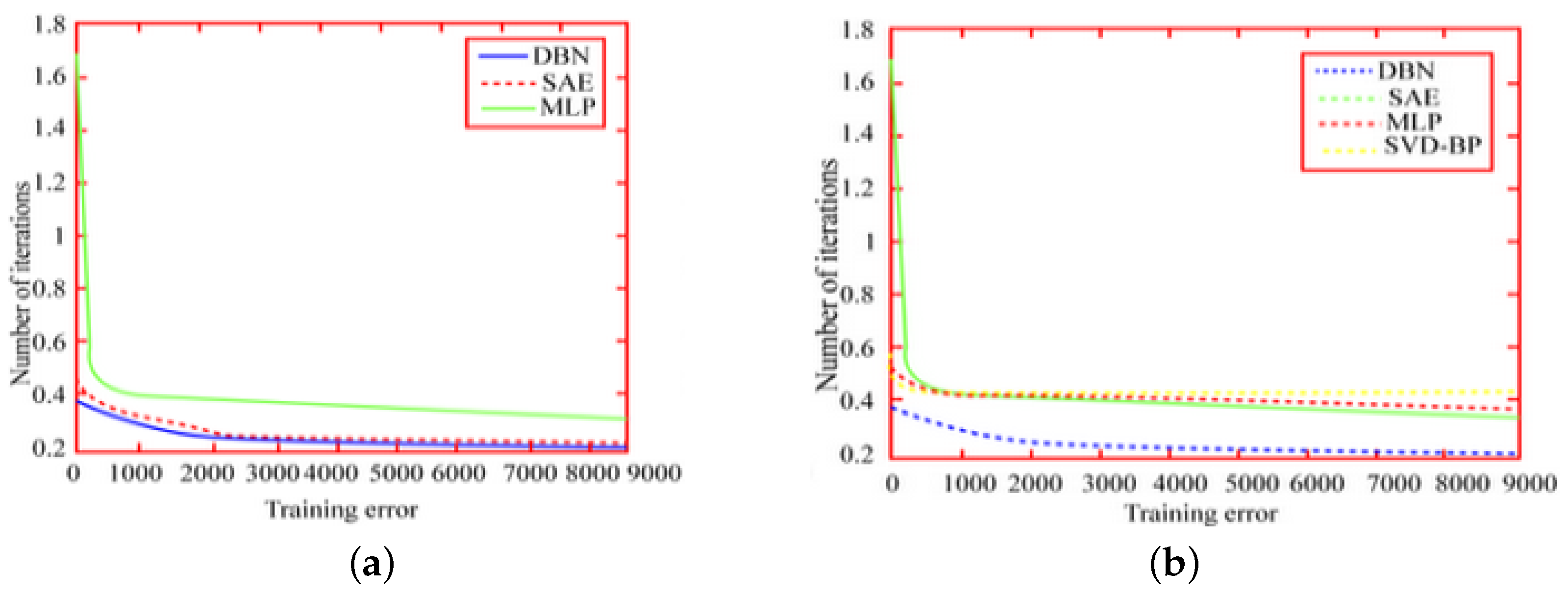
The partial forecasting results of the DL-EWP model shown in Figure 10 demonstrated the superiority of the DL-EWP model. The classification test results showed that all five reference models made a wrong classification of the Elliott wave model 7 of the Euro Index between December 2006 and June 2015 (as shown in Figure 10b). The SAE, MLP, BP network, and PCA-BP models judged it as model 5, while the SVD-BP model judged it as model 6. The training error variation curve (computed as the MSE) of the deep confidence network in the DL-EWP model with the reference models at the stage of completing the classification task is shown in Figure 11.
Figure 11a shows the training error variation curves of the three deep network models in the classification stage. The error curve of the DBN network was smoother than that of the SAE network in the fine-tuning stage, which indicated the superiority of the former’s stability against the latter. The training error variation curve of the MLP network also reflected that the network had a higher stability and convergence speed. However, its final training error was higher than that of the DBN network, which may be caused by the network falling into a local optimum. This demonstrated that the DBN network was more reliable than the MLP network and could effectively improve the local optimum problem caused by using BP algorithms in batch. Figure 11b shows the training error variation curves of the DBN network in the fine-tuning stage and the three shallow network models. The DBN network had a faster convergence speed and a higher accuracy than the three shallow network models. Together, this shows that the DBN network converged faster, had a lower final training error, and had a better smoothness than the reference models during the iterative training for classification.

6. Conclusions and Discussion

Based on our results, we can draw the following conclusions: First, our proposed DBN-based DL-EWP model had a high reliability and could successfully and efficiently identify the corresponding Elliott wave models from financial time series. Second, compared with the five reference models, including deep and shallow network models, the DBN network used in the DL-EWP model had a better performance in terms of stability, convergence speed, accuracy, and feature extraction capability. Third, the DL-EWP model improved the prediction performance of traditional BP network models and multilevel classifiers. Fourth, the DL-EWP financial forecasting model incorporating Elliott’s wave theory reduced the error of the deep network model with stock returns as the decision criterion and improved the accuracy of the deep network model with high-frequency buying and selling as the decision criterion.
The research results of this paper can improve the system of financial risk prevention, early warning, disposal and accountability, and build a long-term mechanism for preventing and resolving financial risks. First, we suggest optimizing the monitoring and analysis mechanism, promoting rule-based expert experience, the automation of monitoring and analysis carried out manually, and focusing the responsibilities of monitoring and analysis positions on the analysis and interpretation of monitoring results; second, we suggest establishing a closed-loop monitoring and analysis process of the preanalysis of regulation rules, policy formulation, policy deconstruction and process coupling, and the continuous monitoring of risk characteristics with the key risk characteristics of business portfolios as the core; third, we suggest sorting out the monitoring data requirements and making full use of the results of the labeling system to provide a data basis for refined monitoring and analysis. Before the regulation rules are formulated, a preanalysis needs to be conducted for the business combinations to be regulated by the relevant regulation policies, and the trial analysis results should be used as the basis for subsequent regulation rule formulation; after the regulation rules are completed, the monitoring and analysis results should be regularly summarized in the form of reports to support risk feature identification and the iterative optimization of monitoring rules. We suggest paying close attention to the risks in key areas, improving the foresight, timeliness, and effectiveness of risk identification, continuing to follow the policy of “stabilizing the overall situation, coordinating, classifying, and precisely dismantling” to prevent and resolve financial risks, suppress the stock of risks, and strictly control the incremental risks. Further deepening the function of early correction and risk disposal of deposit insurance can play the role of an incentive and restraint of the risk difference rate and improves the effect of early correction. The main responsibilities of financial institutions and their shareholders, including the local responsibility and the supervisory responsibility of financial management departments, should be merged to form a joint force for risk disposal and ensure the effective implementation of disposal measures. A sound financial risk accountability mechanism, serious accountability for major financial risks, and effective prevention of moral hazard can also resolutely guard the bottom line against systemic financial risks.
Finally, the DL-EWP model itself still has room for improvement. Research on combining deep learning technology and Elliott’s wave theory can be further strengthened. We hope that better deep learning models (such as residual and fractal networks) can be introduced and examined. In addition, due to the limitation of time, this study could not realize the concept of “fractal level” of Elliott’s wave theory, as Elliott said that cyclic motion is a natural and universal phenomenon. In the future, if neural networks can be effectively integrated with fractal theory and the network structure can reflect the concept of “fractal level”, then it will trigger another leap in neural network technology.

Author Contributions

Investigation, M.S.; Data curation, Y.L.; Writing—original draft, Y.D.; Writing—review & editing, G.J.; Supervision, L.C. All authors have read and agreed to the published version of the manuscript.

Funding

This research received no external funding.

Conflicts of Interest

The authors declare no conflict of interest. The funders had no role in the design of the study; in the collection, analyses, or interpretation of data; in the writing of the manuscript, or in the decision to publish the results.

Abbreviations

The following abbreviations are used in this manuscript:
SAEStacked autoencoder
MLPMultilayer perceptron
BPBackpropagation
PCAPrincipal component analysis
SVDSingular value decomposition
PCA-BPPrincipal component analysis backpropagation
SVD-BPSingular value decomposition backpropagation
DLDeep learning
DL-EWPDeep learning + Elliott wave principle
DNNsDeep neural networks
LSTMLong short-term memory
WASPWave analysis stock prediction
RBMRestricted Boltzmann machine
DBNDeep belief network
MSEMean square error
RMSERoot-mean-square error
MAEMean absolute error
ERError rate
PLR_VIPPiecewise linear representation

References

  1. Huang, D.S.; Han, K.; Hussain, A. High-Frequency Trading Strategy Based on Deep Neural Networks. Lect. Notes Comput. Sci. 2016, 42, 166–178. [Google Scholar]
  2. Chong, E.; Han, C.; Park, F. Deep learning networks for stock market analysis and prediction. Expert Syst. Appl. Int. J. 2017, 83, 187–205. [Google Scholar] [CrossRef] [Green Version]
  3. Fischer, T.; Krauss, C. Deep learning with long short-term memory networks for financial market predictions. Eur. J. Oper. Res. 2018, 270, 654–669. [Google Scholar] [CrossRef] [Green Version]
  4. Bao, W.; Yue, J.; Rao, Y.; Boris, P. A deep learning framework for financial time series using stacked autoencoders and long-short term memory. PLoS ONE 2017, 12, e0180944. [Google Scholar] [CrossRef] [PubMed] [Green Version]
  5. Basu, T.; Menzer, O.; Ward, J.; SenGupta, I. A Novel Implementation of Siamese Type Neural Networks in Predicting Rare Fluctuations in Financial Time Series. Risks 2022, 10, 39. [Google Scholar] [CrossRef]
  6. Navon, D.; Olearczyk, N.; Albertson, R.C. Genetic and developmental basis for fin shape variation in African cichlid fishes. Mol. Ecol. 2017, 26, 291–303. [Google Scholar] [CrossRef] [PubMed]
  7. SenGupta1, I.; Nganje, W.; HansonJie, E. Refnements of Barndorf Nielsen and Shephard Model: An Analysis of Crude Oil Price with Machine Learning. Ann. Data Sci. 2021, 8, 39–55. [Google Scholar] [CrossRef] [Green Version]
  8. Moews, B.; Herrmann, J.M.; Ibikunle, G. Lagged correlation-based deep learning for directional trend change prediction in financial time series. Expert Syst. Appl. 2018, 120, 197–206. [Google Scholar] [CrossRef] [Green Version]
  9. Jarusek, R.; Volna, E.; Kotyrba, M. FOREX rate prediction improved by Elliott waves patterns based on neural networks. Neural Netw. Off. J. Int. Neural Netw. Soc. 2022, 145, 342–355. [Google Scholar] [CrossRef] [PubMed]
  10. Volna, E.; Kotyrba, M.; Jarusek, R. Multi-classifier based on Elliott wave’s recognition. Comput. Math. Appl. 2013, 66, 213–225. [Google Scholar] [CrossRef]
  11. Wen, J.; Fang, X.; Cui, J.; Fei, L.; Yan, K.; Chen, Y.; Xu, Y. Robust Sparse Linear Discriminant Analysis. IEEE Trans. Circuits Syst. Video Technol. 2019, 29, 390–403. [Google Scholar] [CrossRef]
  12. Li, Q.; Jin, J. Evaluation of Foundation Fieldbus H1 Networks for Steam Generator Level Control. IEEE Trans. Control. Syst. Technol. 2011, 19, 1047–1058. [Google Scholar] [CrossRef]
  13. Elaal, M.; Selim, G.; Fakhr, W. Stock Market Trend Prediction Model for the Egyptian Stock Market Using Neural Networks and Fuzzy Logic. In Proceedings of the Bio-Inspired Computing & Applications-International Conference on Intelligent Computing, Lugano, Switzerland, 12–15 December 2022. [Google Scholar]
  14. Atsalakis, G.S.; Tsakalaki, K.I.; Zopounidis, C. Forecasting the Prices of Credit Default Swaps of Greece by a Neuro-fuzzy Technique. Int. J. Econ. Manag. 2012, 4, 45–58. [Google Scholar]
  15. Wen, J.; Xu, Y.; Liu, H. Incomplete Multiview Spectral Clustering With Adaptive Graph Learning. IEEE Trans. Cybern. 2018, 50, 1418–1429. [Google Scholar] [CrossRef] [PubMed]
  16. Shipard, J.; Wiliem, A.; Fookes, C. Does Interference Exist When Training a Once-For-All Network? In Proceedings of the IEEE/CVF Conference on Computer Vision and Pattern Recognition, New Orleans, LA, USA, 18 June–24 June 2022. [Google Scholar]
  17. Zhang, K.; Shi, S.; Liu, S.; Wan, J.; Ren, L. Research on DBN-based Evaluation of Distribution Network Reliability. In Proceedings of the 7th International Conference on Renewable Energy Technologies (ICRET 2021), Kuala Lumpur, Malaysia, 8–10 January 2021; p. 03004. [Google Scholar]
  18. Kathleen, M. Elliott Young. Forever Prisoners: How the United States Made the World’s Largest Immigrant Detention System. Am. Hist. Rev. 2022, 126, 1611–1615. [Google Scholar]
  19. Wen, J.; Xu, Y.; Li, Z.; Ma, Z.; Xu, Y. Inter-class sparsity based discriminative least square regression. Neural Netw. 2018, 102, 36–47. [Google Scholar] [CrossRef] [PubMed]
  20. Wu, C.J.; Zeng, W.S.; Ho, J.M. Optimal Segmented Linear Regression for Financial Time Series Segmentation. In Proceedings of the 2021 International Conference on Data Mining Workshops (ICDMW), Auckland, New Zealand, 7–10 December 2021. [Google Scholar]
  21. Hamzehzarghani, H.; Behjatnia, S.; Delnavaz, S. Segmented linear Model to characterize tolerance to tomato yellow leaf curl virus and tomato leaf curl virus in two tomato cultivars under greenhouse conditions. Iran Agric. Res. 2020, 39, 17–28. [Google Scholar]
  22. Gajera, V.; Shubham; Gupta, R.; Jana, P.K. An effective Multi-Objective task scheduling algorithm using Min-Max normalization in cloud computing. In Proceedings of the 2016 2nd International Conference on Applied and Theoretical Computing and Communication Technology (iCATccT), Bangalore, India, 21–23 July 2016. [Google Scholar]
  23. Dimitrios, D.; Anastasios, P.; Thanassis, K.; Dimitris, K. Do confidence indicators lead Greek economic activity? Bull. Appl. Econ. 2021, 8, 1. [Google Scholar]
  24. Nevela, A.Y.; Lapshin, V.A. Model Risk and Basic Approaches to its Estimation on Example of Market Risk Models. Finans. žhurnal—Financ. J. 2022, 2, 91–112. [Google Scholar] [CrossRef]
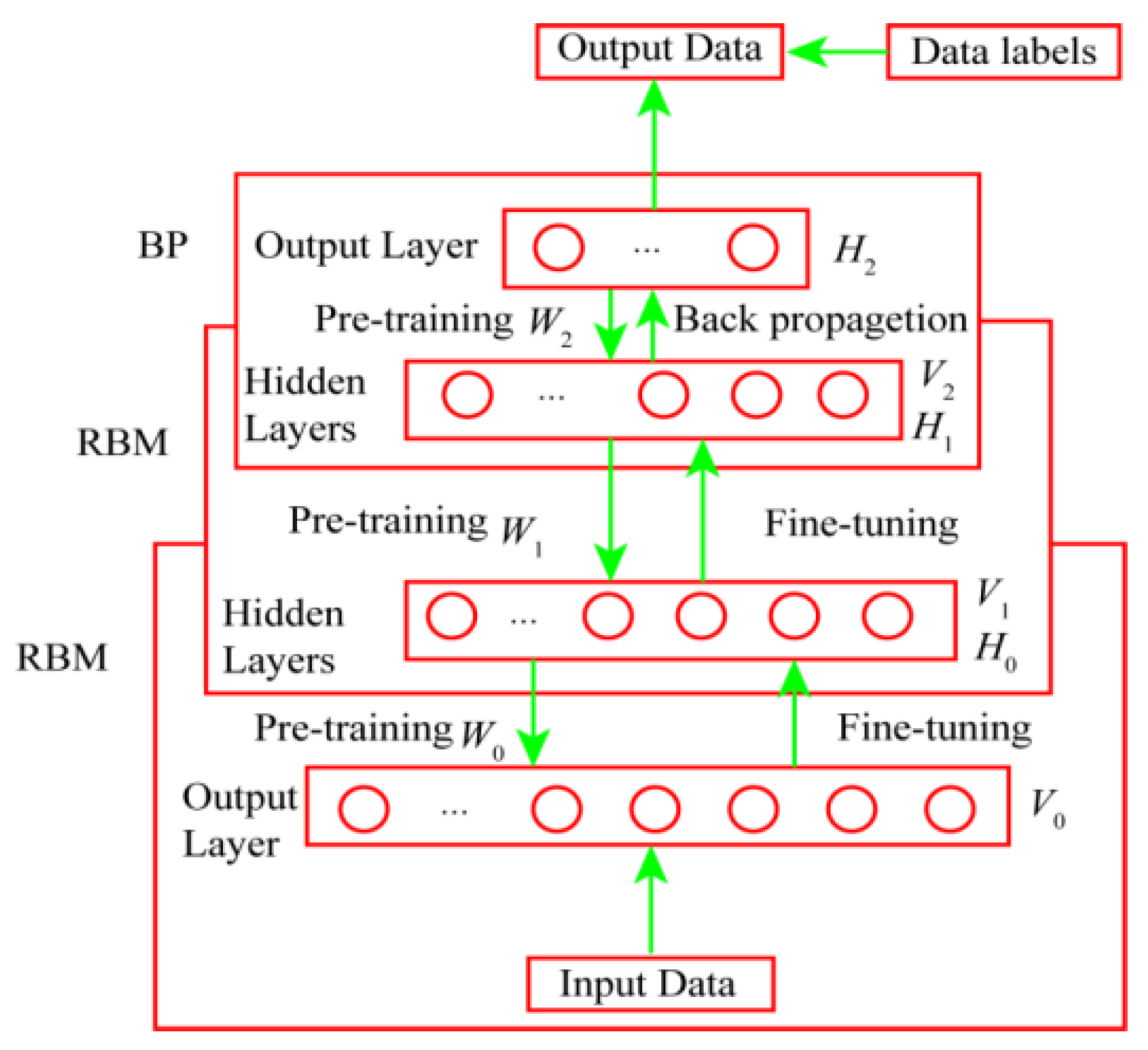
Figure 1. DBN’s classic architecture example.
Mathematics 11 01466 g001
Figure 2. The basic model of the Elliott wave.
Mathematics 11 01466 g002
Figure 3. The basic framework of the DL-EWP model.
Mathematics 11 01466 g003
Figure 4. DL-EWP model.
Mathematics 11 01466 g004
Figure 5. The DBN training algorithm.
Mathematics 11 01466 g005
Figure 6. The basic idea of the PLR_VIP algorithm.
Mathematics 11 01466 g006
Figure 7. Example of data preprocessing. (a) An example of the weekly K-chart of the S&P 500 Index. (b) Unified step size result of PLR_VIP algorithm.
Mathematics 11 01466 g007
Figure 8. Elliott wave basic model.
Mathematics 11 01466 g008
Figure 9. The training error variation curve of the DBN network.
Mathematics 11 01466 g009
Figure 10. Example of prediction results of the DL-EWP model.
Mathematics 11 01466 g010
Figure 11. Training error of the DL-EWP model compared with the reference models in the classification stage. (a) Comparison of the training errors of three deep network models. (b) Comparison of the training errors between the DBN network and three shallow network models.
Mathematics 11 01466 g011
Table 1. Study data.
Foreign Exchange Market Global Stock IndicesCommodities (Futures)
US Dollar IndexDow Jones Industrial Average (U.S.) (“Dow”)COMEX Copper
Euro IndexStandard & Poor’s 500 Index (U.S.) (“S&P”)COMEX Gold
EUR/USDFTSE 100 (UK) (“FTSE 1000”)WTI Crude Oil
EUR/GBPDAX (Germany) (“DAX”)CBOT Soybeans
GBP/USDSSE (China) (“SSE”)CBOT Wheat
USD/CNYHang Seng Index (Hong Kong, China) (“Hang Seng”)ICE Cocoa
Table 2. Basic information about the data.
Market
Category
Trading VarietiesSamples SizeTime Range of DataData Cycle
Foreign
exchange
market
Data Summaries6092
Euro Index5094 January 1971–9 November 2018Season/month/week/day
EUR/USD3374 January 1971–9 November 2018Season/month/week/day
EUR/GBP3734 January 1971–9 November 2018Season/month/week/day
US Dollar Index20119 March 1975–7 November 2018Season/month/week/day
GBP/USD3911 March 1900–9 November 2018Season/month/week/day
USD/CNY649 April 1991–9 November 2018Week/day
Forex Total1875
CommoditiesCMX Copper4211 July 1959–7 November 2018Year/season/month/week/day
CBOT Wheat5041 April 1959–9 November 2018Year/season/month/week/day
ICE Cocoa4911 July 1959–21 November 2018Year/season/month/week/day
CMX Gold5102 June 1969–9 November 2018Season/month/week/day
WTI Crude Oil3171 January 1982–7 November 2018Season/month/week/day
CBOT Soybeans3291 July 1959–9 November 2018Season/month/week/day
Commodity Summaries2572
S&P3561 November 1928–8 November 2018Year/season/month/week/day
Global
stock
indices
FTSE 10057813 November 1935–7 November 2018Year/season/month/week/day
Dow2841 October 1928–2 November 2018Year/season/month/week/day
DAX16428 July 1959–8 November 2018Year/season/month/week/day
SSE14919 December 1990–7 November 2018Season/month/week/day
Hang Seng11419 December 1990–7 November 2018Season/month/week/day
Total Stock Index1645
Table 3. DBN network parameters.
Number of
Hidden Layers
Number of
Hidden Layer Units
Learning
Rate
Number of
Iterations
Momentum
Factor
210/100.1/0.121000/90000.51/0.8
Table 4. Model evaluation methods.
Evaluation CriteriaFormula of Calculation
MSE M S E = 1 n i = 1 n ( T i P i ) 2
RMSE R M S E = 1 n i = 1 n ( T i p i ) 2
MAE M A E = 1 n i = 1 n | T i P i |
ER E R = ( 1 | M o d e l p M o d e l r ) ( 1 | M o d e l p M o d e l r ) × 100 %
Table 5. Network parameters of the SAE model.
Number of
Hidden Layers
Number of
Hidden Layer Units
Learning
Rate
Number of
Iterations
Momentum
Factor
210/100.1/0.12950/90000.51/0.5
Table 6. Network parameters of the MLP model.
Number of
Hidden Layers
Number of
Hidden Layer Units
Learning
Rate
Number of
Iterations
Momentum
Factor
210/100.01590000.6
Table 7. Network parameters of BP network, PCA-BP, and SVD-BP models.
Number of Hidden LayersLearning RateNumber of IterationsMomentum Factor
20.01590000.6
Table 8. Comparison of the prediction performance of the models.
Prediction ModelEvaluation Criteria
MSERMSEMAEER
Deep network modelDL-EWP0.43660.65770.912831.06%
SAE0.43060.65380.939234.74%
MLP0.63490.84071.456243.62%
Shallow network modelBP0.77210.87151.48251.34%
PCA-BP0.70010.82071.309255.55%
SVD-BP0.87450.91981.613579.97%
Disclaimer/Publisher’s Note: The statements, opinions and data contained in all publications are solely those of the individual author(s) and contributor(s) and not of MDPI and/or the editor(s). MDPI and/or the editor(s) disclaim responsibility for any injury to people or property resulting from any ideas, methods, instructions or products referred to in the content.