A Modified q-BFGS Algorithm for Unconstrained Optimization

Abstract

This paper presents a modification of the q-BFGS method for nonlinear unconstrained optimization problems. For this modification, we use a simple symmetric positive definite matrix and propose a new q-quasi-Newton equation, which is close to the ordinary q-quasi-Newton equation in the limiting case. This method uses only first order q-derivatives to build an approximate q-Hessian over a number of iterations. The q-Armijo-Wolfe line search condition is used to calculate step length, which guarantees that the objective function value is decreasing. This modified q-BFGS method preserves the global convergence properties of the q-BFGS method, without the convexity assumption on the objective function. Numerical results on some test problems are presented, which show that an improvement has been achieved. Moreover, we depict the numerical results through the performance profiles.

1. Introduction

There are many methods for solving nonlinear unconstrained minimization problems [1,2,3,4,5], most of them are variants of the Newton and quasi-Newton methods. Newton’s method uses the specification of the Hessian matrix, which is sometimes difficult to calculate, whereas the quasi-Newton method uses an approximation of Hessian. Over time, several attempts have been made to improve the effectiveness of quasi-Newton methods. The BFGS (Broyden–Fletcher–Goldfarb–Shanno) method is a quasi-Newton method for solving nonlinear unconstrained optimization problems, which is developed by Fletcher [6], Goldfarb [7], Shanno [8], and Broyden [9]. Since the 1970s, the BFGS method has become popular and is considered an effective quasi-Newton method. Some researchers have established that the BFGS method achieves global convergence under the assumption of convexity on the objective function. Mascarene has been shown with an example that the standard BFGS method fails with exact line search for non-convex functions [10]. Using inexact line search, some authors [11,12] established that the BFGS method achieves global convergence without the assumption of convexity on the objective function.

Quantum calculus (q-calculus) is a branch of mathematics and does not require limits to derive q-derivatives; therefore, it is also known as calculus without limits. In quantum calculus, we can obtain the q-derivative of a non-differentiable function by replacing the classical derivative with the q-difference operator, and if we take the limit $q\to 1$, then the q-derivative reduces to the classical derivative [13]. Since the 20th century, quantum calculus has been linking physics [14] and mathematics [15] that span from statistical mechanics [16] and quantum theory [17] to hyper-geometric functions and number theory [14]. Quantum analysis was first introduced in the 1740s when Euler wrote in Latin about the theory of partitions, also known as additive analytic number theory.

At the beginning of the 19th century, Jackson generalized the concepts of classical derivatives in the context of q-calculus, known as Jackson’s derivative, or q-derivative operator, or q-difference operator or simply q-derivative [18]. He systematically developed quantum calculus based on pioneer work by Eular and Henie. His work introduced functions, mean value theorems [19], Taylor’s formula and its remainder [20,21], fractional integrals [22], integral inequalities and generalizations of series in the context of q-calculus [23]. The first time Soterroni [24] introduced the q-gradient vector. To obtain this, instead of the classical first order partial derivative, the first order partial q-derivative obtained from the q-difference operator is used.

In unconstrained optimization first time, Soterroni [24] used the q-derivative to establish the q-variant of the steepest descent method. After that, he also introduced the q-gradient method for global optimization [25]. In recent years, some authors have given some numerical techniques in the context of q-calculus to solve nonlinear unconstrained optimization problems [26,27,28]. In these methods, instead of a general gradient, a q-gradient is used because it permits the descent direction to work in the broader set of directions to converse rapidly.

Moreover, optimization has a crucial role in the field of chemical science. In this field, optimization methods have been used to minimize the energy consumption process in plants, design optimum fluid flow systems, optimize product concentration and reaction time in systems, and optimize the separation process in plants [29,30,31]. Some authors [32,33] have shown that the BFGS method is systematically superior in obtaining stable molecular geometries by reducing the gradient norm in a monotonic fashion. In a similar way, the modified q-BFGS algorithm can be used to find stable molecular geometries for large molecules.

In this paper, we modify the q-BFGS method for nonlinear unconstrained optimization problems. For this modification, we propose a new q-quasi-Newton equation with the help of a positive definite matrix, and in the limiting case, our new q-quasi-Newton equation is close to the ordinary q-quasi-Newton equation. Instead of calculating the q-Hessian matrices, we approximate them using only the first order q-derivative of the function. We use an independent parameter $q\in (0,1)$ and quantum calculus based q-Armijo–Wolfe line search [34] to ensure that the objective function value is decreasing. The use of q-gradient in this line search is responsible for escaping the point from the local minimum to the global minimum at each iteration. The proposed method is globally convergent without the convexity assumption on the objective function. Then, numerical results on some test problems are presented to compare the new method with the existing approach. Moreover, we depict the numerical results through the performance profiles.

The organization of this paper is as follows: In Section 2, we recall essential preliminaries related to the q-calculus and the BFGS method. In the next section, we present a modified q-quasi-Newton equation, and using this, we give a modified q-BFGS algorithm and discuss its properties. In Section 4, we present the global convergence of the modified q-BFGS method. In the next section, we present numerical results. Finally, we give a conclusion in the last section.

2. Preliminaries

In this section, we reviewed some important definitions and other prerequisites from q-calculus and nonlinear unconstrained optimization.

Let $q\in (0,1)$, then, a q-complex number is denoted by ${\left[b\right]}_q$ and defined as follows [14]:

$${\left[b\right]}_q=\frac{q^b-1}{q-1},b\in \mathbb{C}.$$

A q-natural number ${\left[m\right]}_q$ is defined as follows [13]:

$${\left[m\right]}_q=1+q+\cdots +q^{m-1},m\in \mathbb{N}.$$

In q-calculus, the q-factorial [14] of a number ${\left[m\right]}_q$ is denoted by ${\left[m\right]}_q!$ and defined as follows:

$${\left[m\right]}_q!={\left[1\right]}_q{\left[2\right]}_q\dots {[m-1]}_q{\left[m\right]}_q,m\in \mathbb{N}$$

and

$${\left[0\right]}_q!=1.$$

The q-derivative $(q\ne 1)$ [18] of a real-valued continuous function $f:\mathbb{R}\to \mathbb{R}$, provided that f is differentiable at 0, is denoted by $D_{q}f$ and defined as follows:

$$D_{q}f\left(x\right)=\left\{\begin{array}{cc}\frac{f\left(x\right)-f\left(qx\right)}{(1-q)x},\hfill & \mathrm{if}x\ne 0\hfill \\ f^{\prime }\left(x\right),\hfill & \mathrm{if}x=0.\hfill \end{array}\right.$$

If provided that f is differentiable on $\mathbb{R}$ then in the limiting case (q→1), the q-derivative is equal to classical derivative.

Let $f:{\mathbb{R}}^n\to \mathbb{R}$ be a real continuous function, then for $x=(x_1,x_2,\dots ,x_n)$∈${\mathbb{R}}^n$, consider an operator ${\epsilon }_{q,i}$ on h as

$$\left({\epsilon }_{q,i}f\right)\left(x\right)=f(x_1,x_2,\dots ,q{x}_i,x_{i+1},\dots ,x_n).$$

The partial q-derivative [22] of f at x with respect to $x_i$, denoted by $D_{q,x_i}f$ and defined as follows:

$$D_{q,x_i}f\left(x\right)=\left\{\begin{array}{cc}\frac{f\left(x\right)-\left({\epsilon }_{q,i}f\right)\left(x\right)}{(1-q)x_i},\hfill & \mathrm{if}{x}_i\ne 0\hfill \\ \frac{\partial f\left(x\right)}{\partial x_i},\hfill & \mathrm{if}{x}_i=0.\hfill \end{array}\right.$$

In the same way, higher order partial q-derivatives are defined as follows:

$$\begin{array}{cc}\hfill D_q^0& =f\left(x\right),\hfill \\ \hfill D_{q,x_1^{k_1},\dots ,x_i^{k_i}\dots ,x_n^{k_n}}^{m}f\left(x\right)& =\left(D_q,x_i\left(D_{q,x_1^{k_1}\dots x_i^{k_i-1},\dots ,x_n^{k_n}}^{m-1}f\right)\right)\left(x\right),\hfill \\ \hfill & \mathrm{where}{k}_1+k_2+\cdots +k_n=m\mathrm{and}m=1,2,\dots ,\hfill \end{array}$$

Then, the q-gradient [24] of f is

$$\left({\nabla }_{q}f\left(x\right)\right)={\left[D_{q,x_1}f\left(x\right),\dots ,D_{q,x_i}f\left(x\right),\dots ,D_{q,x_n}f\left(x\right)\right]}^T.$$

To simplify the presentation, we use $A>0(\ge 0)$ to denote any $n\times n$ symmetric and positive definite (semi-definite) matrix A, use $f:{\mathbb{R}}^n\to \mathbb{R}$ to denote a real-valued function, use $g_q\left(x\right)$ to denote the q-gradient of f at x, use $\left|\right|x\left|\right|$ to denote Euclidean norm of a vector $x\in {\mathbb{R}}^n$, use $A^k$ to denotes the q-quasi-Newton update Hessian at $x^k$, throughout this paper.

Let $f:{\mathbb{R}}^n\to \mathbb{R}$ be continuously q-derivative then consider the following unconstrained optimization problem:

$$\begin{array}{c}\hfill \underset{x\in {\mathbb{R}}^n}{min}f\left(x\right).\end{array}$$

(1)

The q-BFGS method [34] generates a sequence $\left\{x^k\right\}$ by the following iterative scheme:

$$\begin{array}{c}\hfill x^{k+1}=x^k+{\alpha }^k{d}_q^k;k\in \left\{0\right\}\cup \mathbb{N},\end{array}$$

(2)

where ${\alpha }^k$ and $d_q^k$ are step length and q-BFGS descent direction, respectively.

The q-BFGS descent direction is obtained by solving the following linear equation:

$$\begin{array}{c}\hfill g_q^k+A^k{d}_q^k=0,\end{array}$$

(3)

where $A^k$ is the q-quasi-Newton update Hessian. The sequence $A^k$ satisfies the following equation:

$$A^{k+1}{\delta }^k={\gamma }^k,$$

where ${\delta }^k=x^{k+1}-x^k$ and ${\gamma }^k=g_q^{k+1}-g_q^k.$ In the context of q-calculus, we refer to the Broyden–Fletcher–Goldfarb–Shanno (BFGS) update formula as the q-BFGS update formula. Thus, the Hessian $A^k$ is updated by the following q-BFGS formula:

$$\begin{array}{c}\hfill A^{k+1}=A^k-\frac{A^k{\delta }^k{\left({\delta }^k\right)}^T{A}^k}{{\left({\delta }^k\right)}^T{A}^k{\delta }^k}+\frac{{\gamma }^k{\left({\gamma }^k\right)}^T}{{\left({\delta }^k\right)}^T{\gamma }^k},\end{array}$$

(4)

3. Modified q-BFGS Algorithm

We modify the q-BFGS algorithm using the following function [35]:

$$\begin{array}{c}\hfill f_k\left(x\right)=f\left(x\right)+\frac{1}{2}{(x-x^k)}^T{B}^k(x-x^k),\end{array}$$

where $B^k$ is a positive definite symmetric matrix. We obtain the following new q-quasi-Newton equation by using the function $f_k$ to the q-quasi-Newton method in the kth iterate:

$$\begin{array}{c}\hfill A^{k+1}{\delta }^k={\lambda }^k,\end{array}$$

(5)

where ${\lambda }^k={\gamma }^k+B^k{\delta }^k.$ If we take k $\to \infty$ and ${\delta }_k\to 0$, our new q-quasi-Newton equation is similar to the ordinary q-quasi-Newton equation. Using the above modification of the q-BFGS formula, we obtain the new one as follows:

$$\begin{array}{c}\hfill A^{k+1}=A^k-\frac{A^k{\delta }^k{\left({\delta }^k\right)}^T{A}^k}{{\left({\delta }^k\right)}^T{A}^k{\delta }^k}+\frac{{\lambda }^k{\left({\lambda }^k\right)}^T}{{\left({\delta }^k\right)}^T{\lambda }^k},\end{array}$$

(6)

where ${\lambda }^k={\gamma }^k+B^k{\delta }^k.$

To provide a better formula, the primary task of this research is to determine how to select a suitable $B^k$. We direct our attention to finding $B^k$ as a simple structure that carries some second order information of objective function. In this part, we will discuss a new choice of f and assume it to be sufficiently smooth.

Using the following quadratic model for the objective function [36,37], we have

$$\begin{array}{c}\hfill f\left(x\right)\simeq f\left(x^{k+1}\right)+{\left(g_q^{k+1}\right)}^T(x-x^{k+1})+\frac{1}{2}{(x-x^{k+1})}^T{G}^{k+1}(x-x^{k+1}),\end{array}$$

(7)

where $G^{k+1}$ denotes a Hessian matrix at point $x^{k+1}.$

Hence,

$$\begin{array}{c}\hfill f\left(x^k\right)\simeq f\left(x^{k+1}\right)-{\left(g_q^{k+1}\right)}^T{\delta }^k+\frac{1}{2}{\left({\delta }^k\right)}^T{G}^{k+1}{\delta }^k.\end{array}$$

(8)

Therefore,

$$\begin{array}{cc}\hfill {\left({\delta }^k\right)}^T{G}^{k+1}{\delta }^k& \simeq 2(f^k-f^{k+1}+{\left(g_q^{k+1}\right)}^T{\delta }^k),\hfill \\ \hfill & =2(f^k-f^{k+1})+{(g_q^{k+1}+g_q^k)}^T{\delta }^k+{\left({\delta }^k\right)}^T{\gamma }^k,\hfill \end{array}$$

(9)

where $f^k$ denotes the value of f at $x^k.$

By using (5), we have

$$\begin{array}{c}\hfill {\left({\delta }^k\right)}^T{A}^{k+1}{\delta }^k={\left({\delta }^k\right)}^T{\lambda }^k={\left({\delta }^k\right)}^T{\gamma }^k+{\left({\delta }^k\right)}^T{B}^k{\delta }^k.\end{array}$$

(10)

The combination of Equations (9) and (10) shows that the reasonable choice of $B^k$ should satisfied the following new q-quasi-Newton equation:

$$\begin{array}{c}\hfill {\left({\delta }^k\right)}^T{B}^k{\delta }^k={\mu }^k({\mu }^k=2(f^k-f^{k+1})+{(g_q^{k+1}+g_q^k)}^T{\delta }^k).\end{array}$$

(11)

Theorem 1.

Assume that $B^k$ satisfies (11) and $A^k$ is generated by (6), then for any k,

$$\begin{array}{c}\hfill f\left(x^k\right)=f\left(x^{k+1}\right)+{\left(g_q^{k+1}\right)}^T(x^k-x^{k+1})+\frac{1}{2}{(x^k-x^{k+1})}^T{A}^{k+1}(x^k-x^{k+1}).\end{array}$$

(12)

Proof. 

The conclusion follows immediately using Equations (10) and (11). □

The function f holds the Equation (12) without any convexity assumption on it and any formula derived from the original quasi-Newton equation fails to satisfy the Equation (12). From Equation (11), a choice of $B^k$ can be defined as follows :

$$\begin{array}{c}\hfill B^k{\delta }^k={\eta }^k,\left({\eta }^k=\frac{{\mu }^k}{{\left({\delta }^k\right)}^T{v}^k}{v}^k\right).\end{array}$$

(13)

In above Equation (13), $v^k$ is some vector such that ${\left({\delta }^k\right)}^T{v}^k\ne 0$.

By the Equations (2) and (3), we know that if ${\delta }^k=0$ then $g_q^k=0$. Therefore, for all k we can always assume that $\parallel {\delta }^k\parallel \ne 0$; otherwise, at the $k^{th}$ iteration, the algorithm terminates. Hence, we can choose $v^k={\delta }^k$. Taking $v^k={\delta }^k$ in the Equation (10), we have a choice of $B^k$ as follows:

$$\begin{array}{c}\hfill B^k=\frac{{\mu }^k}{\parallel {\delta }^k{\parallel }^2}I,\end{array}$$

(14)

where the norm is the Euclidean norm and ${\mu }^k=2(f^k-f^{k+1})+{(g_q^{k+1}+g_q^k)}^T{\delta }^k.$

Remark 1.

The structure of $B^k$ is very simple, so we can construct and analyze it easily. We only need to consider the value of $B^k{\delta }^k$ to calculate the modified $A^{k+1}$ from the modified quasi-Newton Equation (5). Thus, once $v^k$ is fixed, different choices of $B^k$, which satisfied (13) gives the same $A^{k+1}$.

For computing the step length following q-gradient based modified Armijo–Wolfe line search conditions [34] are used:

$$\begin{array}{c}\hfill f(x^k+{\alpha }^k{d}_q^k)\le f\left(x^k\right)+{\sigma }_1{\alpha }^k{\left(d_q^k\right)}^T{g}_q^k,\end{array}$$

(15)

and

$$\begin{array}{c}\hfill {\nabla }_{q}f{(x^k+{\alpha }^k{d}_q^k)}^T{d}_q^k\ge {\sigma }_2{\left(d_q^k\right)}^T{g}_q{}^k,\end{array}$$

(16)

where $0<{\sigma }_1<{\sigma }_2<1$. Additionally, if ${\alpha }^k$ = 1 satisfies (16), we take ${\alpha }^k$ = 1. In the above line search, a sufficient reduction in the objective function and nonacceptance of short step length is ensured by (15) and (16), respectively.

A good property of Formula (6) is that $A^{k+1}$ inherits the positive definiteness of $A^k$ as long as ${\left({\delta }^k\right)}^T{\lambda }^k>0$; provided that f is convex and step length is computed by an above line search. However,  when f is a non-convex function, then the above line search does not ensure the condition ${\left({\delta }^k\right)}^T{\lambda }^k>0$. Hence, in this case, $A^{k+1}$ is not necessarily positive definite even if $A^k$ is positive definite. Therefore, some extra caution updates should be introduced as follows:

Define the index set K as follows:

$$\begin{array}{c}\hfill K=\left\{k:\frac{{\left({\delta }^k\right)}^T{\lambda }^k}{\parallel {\delta }^k{\parallel }^2}\ge ϵ\parallel g_q^k{\parallel }^c\right\},\end{array}$$

(17)

where $\beta \in [{\vartheta }_1,{\vartheta }_2]$, with $0<{\vartheta }_1\le {\vartheta }_2$ and $ϵ$ are positive constants. We determine $A^{k+1}$ by the following rule:

$$A^{k+1}=\left\{\begin{array}{cc}{A}^k-\frac{A^k{\delta }^k{\left({\delta }^k\right)}^T{A}^k}{{\left({\delta }^k\right)}^T{A}^k{\delta }^k}+\frac{{\lambda }^k{\left({\lambda }^k\right)}^T}{{\left({\delta }^k\right)}^T{\lambda }^k}\hfill & \mathrm{if}\mathrm{k}\in \mathrm{K}\hfill \\ A^k\hfill & \mathrm{if}\mathrm{k}\notin \mathrm{K}.\hfill \end{array}\right.$$

(18)

Corollary 1.

Let $B^k$ be chosen such Equation (13) holds and $A^k$ is generated by (18), then $A^{k+1}>0$, $\forall k\in \mathbb{N}$$\cup \left\{0\right\}$.

Proof. 

Without loss of generality, let $\parallel g^k\parallel \ne 0,\forall k.$ We use mathematical induction on k to prove this corollary. Since $B^0$ is chosen as a positive definite symmetric matrix, the result holds for $k=0$. Let’s assume that the result holds for k = n. We consider the case when $k=n+1$. If $k\in K$, then from Equations (17) and (18), ${\left({\delta }^k\right)}^T{\lambda }^k>0$ holds. Hence, for $k=n+1$, the result also holds. If $k\notin K$, then by our assumption, $A^{k+1}=A^k$ is also positive definite. This completes the proof. □

From the above modifications, we introduce the following Algorithm 1:

Algorithm 1 Modified q-BFGS algorithm

Require:  Objective function $f:{\mathbb{R}}^n\to \mathbb{R}$, $ϵ$ is tolerance for convergence. Select an initial point $x^0\in {\mathbb{R}}^n$, fix $q\in (0,1),$ and an initial positive definite symmetric matrix $A^o\in {\mathbb{R}}^{n\times m}.$ Ensure:  With the corresponding objective value $f\left(x^{*}\right)$, the minimizer $x^{*}$ is encountered. 1: Set $A^0=I_n.$ 2: for k = 0,1,2... do 3:     if $\parallel g_q^k\parallel <ϵ$ then 4:         Stop. 5:     else 6:         Solve the Equation (3) to find a q-descent direction $d_q^k$. 7:         Find a step length ${\alpha }^k$ satisfying Equations (15) and (16). 8:     end if 9:     Compute $x^{k+1}=x^k+{\alpha }^k{d}_q^k$ and using the following equation, calculate $B^k$: $$B^k=\frac{{\mu }^k}{\parallel {\delta }^k{\parallel }^2}I,$$ where the norm is the Euclidean norm and $${\mu }^k=2(f^k-f^{k+1})+{(g_q^{k+1}+g_q^k)}^T{\delta }^k.$$ 10:     Select two appropriate constants $\beta$, $ϵ$, then update $A^{k+1}$ by (18). 11: end for

4. Analysis of the Convergence

Under the following two assumptions, the global convergence [11] of the modified q-BFGS algorithm is shown in this section.

Assumption 1.

The level set

$$\Omega =\{x\in {\mathbb{R}}^n|f\left(x\right)\le f\left(x^0\right)\}$$

is bounded.

Assumption 2.

The function f is continuously q-derivative on Ω, and there exist a constant (Lipschitz constant) $L>0$, such that

$$\begin{array}{c}\hfill \parallel g_q\left(x_1\right)-g_q\left(x_2\right)\parallel \le L\left|\right|x_1-x_2\left|\right|,\forall x_1,x_2\in \Omega .\end{array}$$

(19)

Since $\left\{f^k\right\}$ is a decreasing sequence, it is clear that the sequence $\left\{x^k\right\}$ generated by the modified q-BFGS algorithm is contained in $\Omega$ .

To establish the global convergence of the modified q-BFGS algorithm in the context of q-calculus, first, we show the following lemma:

Lemma 1.

Let Assumptions 1 and 2 hold for f and with $q\in (0,1)$, $\left\{x^k\right\}$ be generated by Algorithm 1. If there exist positive constants $a_1$ and $a_2$ such that the following inequalities:

$$\begin{array}{c}\hfill \parallel A^k{\delta }^k\parallel \le a_1\parallel {\delta }^k\parallel and{\left({\delta }^k\right)}^T{A}^k{\delta }^k\ge a_2{\parallel {\delta }^k\parallel }^2,\end{array}$$

(20)

holds for infinitely many k, then we have

$$\begin{array}{c}\hfill \underset{k\to \infty }{lim}\inf \parallel g_q\left(x^k\right)\parallel =0\end{array}$$

(21)

Proof. 

Using Equations (2) and (3) in (20), we have

$$\begin{array}{c}\hfill a_2\parallel d_q^k\parallel \le \parallel g_q^k\parallel \le a_1\parallel d_q^k\parallel \mathrm{and}{\left(d_q^k\right)}^T{A}^k{d}_q^k\ge a_2{\parallel d_q^k\parallel }^2.\end{array}$$

(22)

We consider a new case using the q-Armijo type line search (15) with backtracking parameter $\rho \in (0,1)$. If ${\alpha }^k\ne 1$, then we have

$$\begin{array}{c}\hfill {\sigma }_1{\rho }^{-1}{\alpha }^k{g_q\left(x^k\right)}^T{d}_q^k<f(x^k+{\rho }^{-1}{\alpha }^k{d}_q^k)-f\left(x^k\right).\end{array}$$

(23)

By the q-mean value theorem [19], there is a ${\theta }^k\in (0,1)$ such that

$$f(x^k+{\rho }^{-1}{\alpha }^k{d}_q^k)-f\left(x^k\right)={\rho }^{-1}{\alpha }^k{g_q(x^k+{\theta }^k{\rho }^{-1}{\alpha }^k{d}_q^k)}^T{d}_q^k,$$

that is,

$$f(x^k+{\rho }^{-1}{\alpha }^k{d}_q^k)-f\left(x^k\right)={\rho }^{-1}{\alpha }^k{g_q\left(x^k\right)}^T{d}_q^k+{\rho }^{-1}{\alpha }^k{\left(g_q(x^k+{\theta }^k{\rho }^{-1}{\alpha }^k{d}_q^k)-g_q\left(x^k\right)\right)}^T{d}_q^k.$$

From Assumption 2, we obtain

$$\begin{array}{c}\hfill f(x^k+{\rho }^{-1}{\alpha }^k{d}_q^k)-f\left(x^k\right)\le {\rho }^{-1}{\alpha }^k{g_q\left(x^k\right)}^T{d}_q^k+L{\rho }^{-2}{\left({\alpha }^k\right)}^2{\parallel d_q^k\parallel }^2.\end{array}$$

(24)

From (23) and (24), we obtain for any $k\in K$

$${\alpha }^k\ge \frac{-(1-{\sigma }_1)\rho g_q^k{\left(x^k\right)}^T{d}_q^k}{L\parallel d_q^k{\parallel }^2}.$$

Since $-g_q\left(x^k\right)=A^k{d}_q^k,$

$${\alpha }^k\ge \frac{(1-{\sigma }_1)\rho {\left(d_q^k\right)}^T{A}^k{d}_q^k}{L\parallel d_q^k{\parallel }^2}.$$

Using (22) in the above inequality, we obtain

$$\begin{array}{c}\hfill {\alpha }^k\ge min\{1,(1-{\sigma }_1)a_2{L}^{-1}\rho \}>0.\end{array}$$

(25)

We consider the case where line search (16) is used; then, from Assumption 2 and from the inequality (16), we obtain the following:

$$({\sigma }_2-1)g_q{\left(x^k\right)}^T{d}_q^k\le {(g_q(x^k+{\alpha }^k{d}_q^k)-g_q\left(x^k\right))}^T{d}_q^k\le L{\alpha }^k{\parallel d_q^k\parallel }^2.$$

The above inequality implies that

$${\alpha }^k\ge \frac{({\sigma }_2-1)g_q{\left(x^k\right)}^T{d}_q^k}{L\parallel d_q^k{\parallel }^2}.$$

Since $-g_q^k=A^k{d}_q^k$,

$${\alpha }^k\ge \frac{-({\sigma }_2-1){\left(d_q^k\right)}^T{A}^k{d}_q^k}{L\parallel d_q^k{\parallel }^2}.$$

Since $A^k{d}_q^k\ge a_2{\parallel d_q^k\parallel }^2,$

$$\begin{array}{c}\hfill {\alpha }^k\ge min\{1,(1-{\sigma }_2)a_2{L}^{-1}\rho \}>0.\end{array}$$

(26)

The inequalities (25) and (26) together show that ${\left\{{\alpha }_k\right\}}_{k\in K}$ is bounded below away from zero whenever line search (16) and (15) are used. Moreover,

$$\begin{array}{cc}\hfill \sum _{k=0}^{\infty }[f\left(x^k\right)-f\left(x^{k+1}\right)]& =\underset{i\to \infty }{lim}\sum _{k=1}^i[f\left(x^k\right)-f\left(x^{k+1}\right)],\hfill \\ \hfill & =f\left(x^1\right)-\underset{i\to \infty }{lim}f\left(x^j\right).\hfill \end{array}$$

That is,

$$\begin{array}{c}\hfill \sum _{k=0}^{\infty }[f\left(x^k\right)-f\left(x^{k+1}\right)]=f\left(x^1\right)-f\left(x^{*}\right).\end{array}$$

This gives the following result

$$\begin{array}{c}\hfill \sum _{k=1}^{\infty }[f\left(x^k\right)-f\left(x^{k+1}\right)]<\infty .\end{array}$$

The above inequality, together with (15) gives,

$$\begin{array}{c}\hfill -\sum _{k=1}^{\infty }{\alpha }^k{\left(g_q^k\right)}^T{d}_q^k<\infty .\end{array}$$

Since $g_q^k=-A^k{d}_q^k,$

$$\begin{array}{c}\hfill \underset{k\to \infty }{lim}{\left(d_q^k\right)}^T{A}^k{d}_q^k=-\underset{k\to \infty }{lim}{\left(g_q^k\right)}^T{d}_q^k\to 0.\end{array}$$

The above result, together with (22), implies (21). □

From the above Lemma 1, we can say that to establish the global convergence of Algorithm 1, it is sufficient to show that there are positive constants $a_1$ and $a_2$ such that the (20) holds for infinitely many k. To prove this, we need the following lemma [34]:

Lemma 2.

Let $A^0$ be a positive definite and symmetric matrix and $A^k$ be updated by (18). Suppose that there exist positive constant m < M such that, for each $k\ge 0,{\lambda }^k$ and ${\delta }^k$ satisfy

$$\begin{array}{c}\hfill \frac{{\left({\delta }^k\right)}^T{\lambda }^k}{\parallel {\delta }^k{\parallel }^2}\ge m\mathit{and}\frac{\parallel {\lambda }^k{\parallel }^2}{{\left(\delta \right)}^T{\lambda }^k}\le M.\end{array}$$

(27)

Then, there exist constants $a_1,a_2>0$ such that for any positive integer t, (20) holds for at least $\lceil \frac{t}{2}\rceil$ values of $k\in \{1,2,\dots ,t\}.$

By using Lemma 2 and Lemma 1, we can prove the following global convergence theorem for Algorithm 1.

Theorem 2.

Let f satisfy Assumption 1 and Assumption 2, and $\left\{x^k\right\}$ be generated by modified q-BFGS Algorithm 1, then the Equation (21) is satisfied.

Proof. 

By using Lemma 1, it is sufficient to show that there are infinitely many k which satisfies (20).

If the set K is finite, then after a finite number of iterations, $A^k$ remains constant. Since matrix, $A^k$ is positive definite and symmetric for each k, and it is clear that there are positive constants $a_1$ and $a_2$ such that Equation (20) holds for all sufficiently large k.

Now, consider the case when K is an infinite set. We go forward by contradiction and assume that (21) is not true. Then, there exists a positive constant α such that $\parallel g_q^k\parallel >\alpha ,\forall k.$

Then, from (17)

$${\left({\delta }^k\right)}^T{\lambda }^k\ge ϵ{\alpha }^{\beta }{\parallel {\delta }^k\parallel }^2,\forall k\in K$$

$$\Rightarrow \frac{1}{{\left({\delta }^k\right)}^T{\lambda }^k}\le \frac{1}{ϵ{\alpha }^{\beta }{\parallel {\delta }^k\parallel }^2},\forall k\in K,$$

$$\Rightarrow \frac{\parallel {\lambda }^k{\parallel }^2}{{\left({\delta }^k\right)}^T{\lambda }^k}\le \frac{\parallel {\lambda }^k{\parallel }^2}{ϵ{\alpha }^{\beta }{\parallel {\delta }^k\parallel }^2},\forall k\in K.$$

From (19), we know that $\parallel {\lambda }^k{\parallel }^2\le L^2{\parallel {\delta }^k\parallel }^2.$ Thus, combining it with the above inequality, we obtain

$$\frac{\parallel {\lambda }^k{\parallel }^2}{{\left({\delta }^k\right)}^T{\lambda }^k}\le \frac{L^2}{ϵ{\alpha }^{\beta }},\forall k\in K.$$

Let $\frac{L^2}{ϵ{\alpha }^{\beta }}=M,$ then

$$\frac{\parallel {\lambda }^k{\parallel }^2}{{\left({\delta }^k\right)}^T{\lambda }^k}\le M,\forall k\in K.$$

Applying Lemma 2 to the matrix subsequence ${\left\{A^k\right\}}_{k\in K}$, we conclude that there exist constants $a_1,a_2>0$ such that the Equation (20) holds for infinitely many k. The proof is then complete. □

The above Theorem 2 shows that the modified q-BFGS algorithm is globally convergent even if convexity is not assumed for f [34].

5. Numerical Results

This section presents the comparison of numerical results obtained with the modified q-BFGS algorithm 1, the q-BFGS algorithm [34], and the BFGS Algorithm [38] for solving a collection of unconstrained optimization problems taken from [39]. For each test problem, we chose an initial matrix as a unit matrix, i.e., $A^0=I.$ Our numerical results are performed on Python3.7 (Google colab). Throughout this section ‘NI’, ‘NF’, and ‘NG’ indicate the total number of iterations, the total number of function evaluations, and the total number of gradient evaluations, respectively. For each test problem, the parameters are common to modified q-BFGS, q-BFGS, and BFGS algorithms. We set $q=0.9999999$, ${\sigma }_1=0.0001$, and ${\sigma }_2=0.9$, and used the condition $\parallel g_q^k\parallel \le {10}^{-6}$ as the stopping criteria. Moreover, we set the parameter $\beta =3$, when $\parallel g_q^k\parallel \le {10}^{-6}$ otherwise we take $\beta =0.01$. In general, we take $q\to 1$ and $q\ne 1$. When $q\ne 1$, then the q-gradient can make any angle with the classical gradient and the search direction can point in any direction.

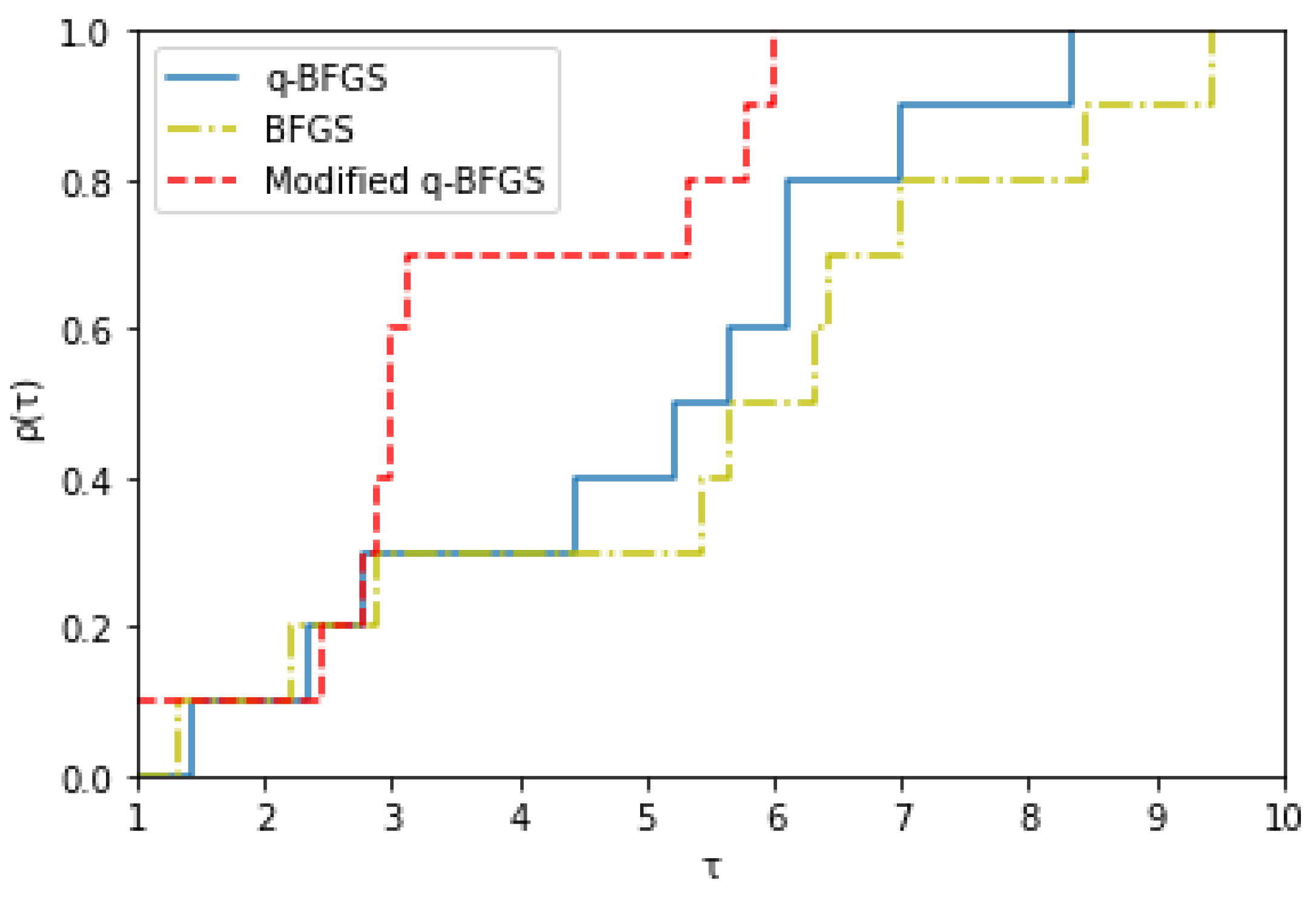
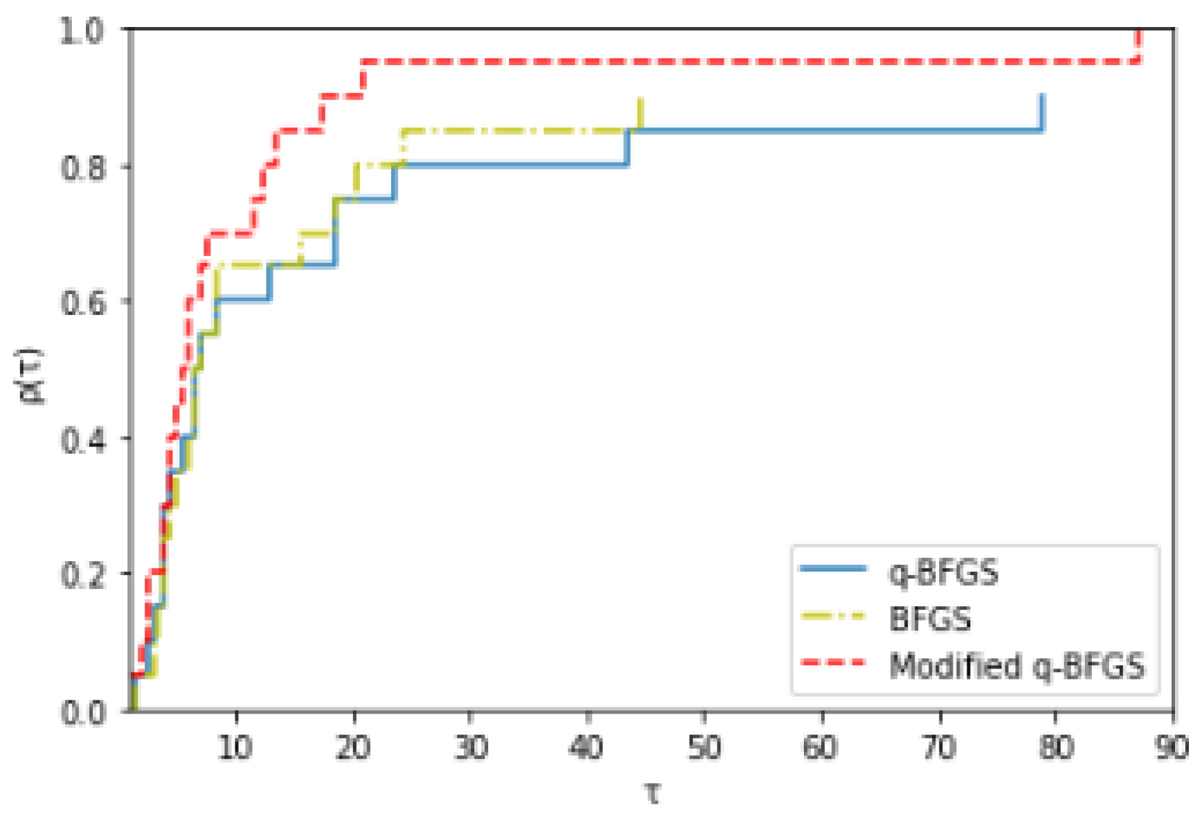
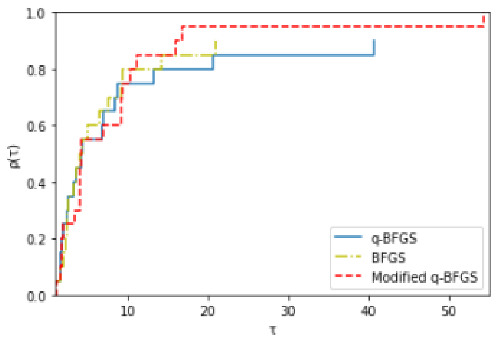
We have used performance profiles for evaluating and comparing the performance of algorithms on a given set of test problems through graphs. Dolan and More [40], presented an appropriate technique to demonstrate the performance profiles, which is a statistical process. We use this as an evaluation tool to show the performance of the algorithm. We are interested in using the number of the iteration, function evaluations, and q-gradient evaluations as the performance measure. The performance ratio is presented as

$$\begin{array}{c}\hfill {\rho }_{p,s}=\frac{r_{(p,s)}}{min\{r_{(p,s)}:1\le r\le n_s\}},\end{array}$$

(28)

Here, $r_{(p,s)}$ refers to the number of the iteration, function evaluations, and q-gradient evaluations, respectively, required to solve problem p by solver s and $n_s$ refers to the number of problems in the model test. The cumulative distribution function is expressed as

$$p_s\left(\tau \right)=\frac{1}{n_p}\mathrm{size}\{p\in {\rho }_{p,s}\le \tau \}$$

where $p_s\left(\tau \right)$ is the probability that a performance ratio ${\rho }_{p,s}$ is within a factor of $\tau$ of the best possible ratio. That is, for a subset of the methods being analyzed, we plot the fraction $p_s\left(\tau \right)$ of problems for which any given method is within a factor $\left(\tau \right)$ of the best. Now we take the following examples to show the computational results:

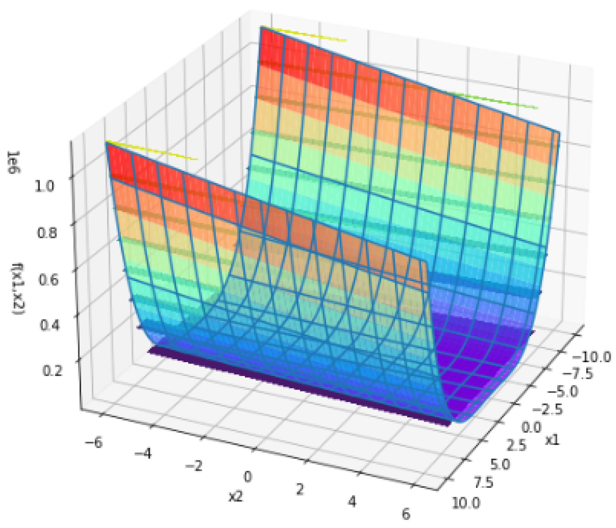
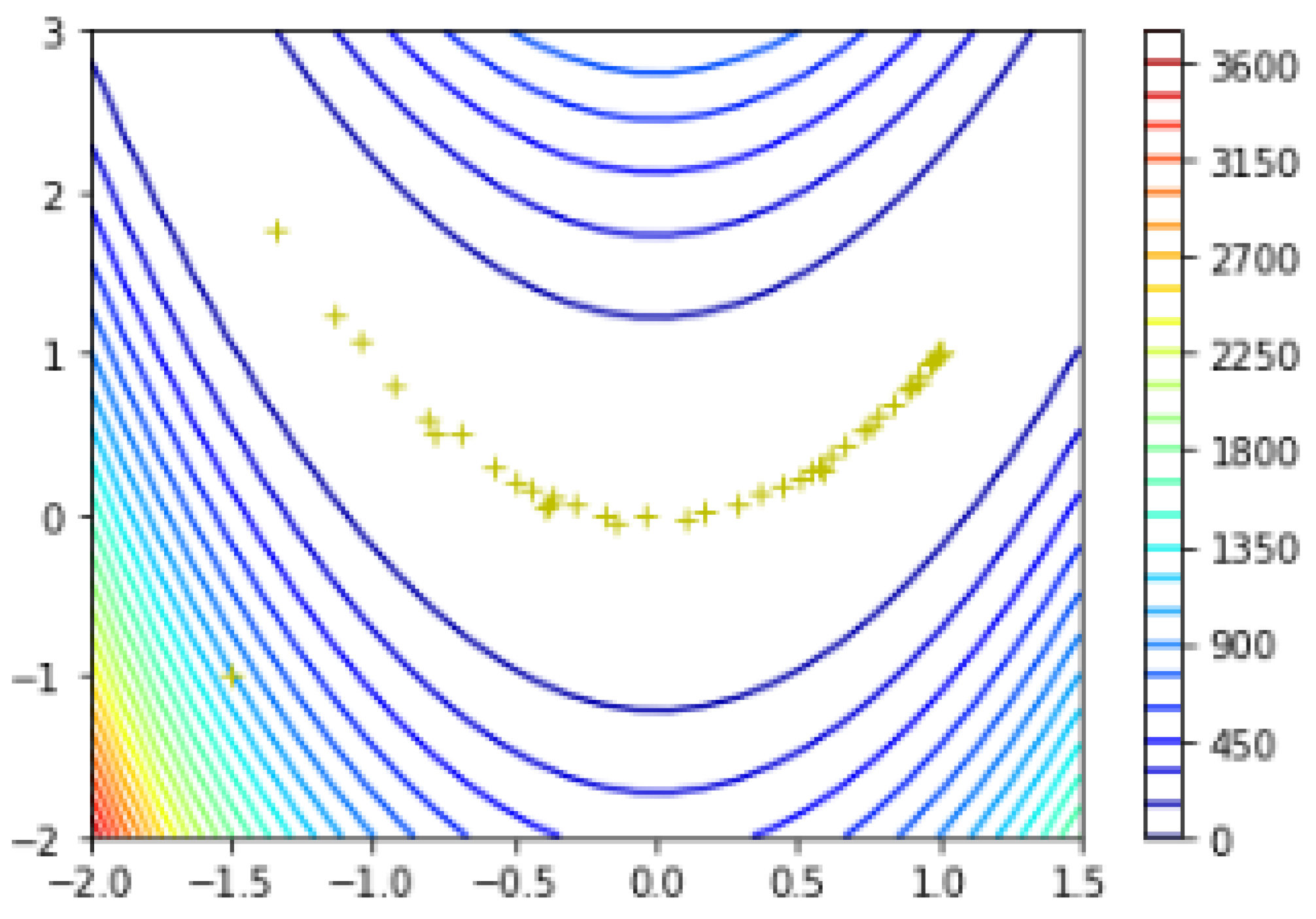
Example 1.

Consider the non-convex Rosenbrock function $f:{\mathbb{R}}^2\to \mathbb{R}$ such that

$$\begin{array}{c}\hfill f(x_1,x_2)=100{(x_2-{x_1}^2)}^2+{(x_1-1)}^2.\end{array}$$

Following Figure 1 represents the surface plot of the Rosenbrock function:

Figure 1. Surface plot of Rosenbrock function.

The Rosenbrock function was introduced by Rosenbrock in 1960. We tested modified q-BFGS, q-BFGS, and BFGS algorithms for 10 different initial points. Numerical results for the Rosenbrock function are given in the following Table 1:

Table 1. Comparison of numerical results of Modified q-BFGS, q-BFGS, and BFGS algorithms for the Rosenbrock function.

S.No.	${\mathit{x}}^0$	Modified q-BFGS	q-BFGS	BFGS
		NI/NF/NG	NI/NF/NG	NI/NF/NG
1	${(-1.5,-1)}^T$	25/95/47	47/198/66	49/213/71
2	${(0,0)}^T$	22/77/35	21/78/26	20/75/25
3	${(-4,4)}^T$	27/125/73	63/82/246	63/255/85
4	${(-3,0)}^T$	28/118/64	55/210/70	58/210/70
5	${(10,0)}^T$	54/197/91	40/150/50	85/372/120
6	${(7,-7)}^T$	52/184/82	75/294/98	76/414/134
7	${(4,5)}^T$	48/174/80	51/201/67	51/198/66
8	${(-2,-2)}^T$	26/112/62	55/201/67	57/342/110
9	${(1,1.2)}^T$	9/38/22	13/57/19	12/93/27
10	${(0,4)}^T$	27/113/61	25/96/32	26/114/38

The Rosenbrock function converges to $x^{*}={(1,1)}^T$ with value $f\left(x^{*}\right)=0$, for the above starting points $x^0$. Figure 2, Figure 3, and Figure 4 show the Dolan and More performance profiles of modified q-BFGS, q-BFGS, and BFGS algorithms for the Rosenbrock function, respectively.

Figure 2. Performance profile based on number of iterations.

Figure 3. Performance profile based on number of gradient evaluations.

Figure 4. Performance profile based on number of function evaluations.

The global minima and plotting points of the Rosenbrock function using the modified q-BFGS algorithm can also be observed in Figure 5.

Figure 5. Global minima of the Rosenbrock function using modified q-BFGS algorithm.

For the starting point $x^0=(-1.5,-1)$, the Rosenbrock function converges to

$$\begin{array}{cc}\hfill & x^{*}={[0.999999996685342,0.999999997414745]}^T,\hfill \\ & \mathrm{with}\hfill \\ & f\left(x^{*}\right)=1.64642951315324e^{-15}\mathrm{and}{\nabla }_{q}f\left(x^{*}\right)={[-1.66435354e^{-06},7.98812111e^{-07}]}^T,\hfill \end{array}$$

in 25 iterations.

The global minima and plotting points of the Rosenbrock function using the q-BFGS algorithm can also be observed in Figure 6.

Figure 6. Global minima of the Rosenbrock function using q-BFGS algorithm [34].

For the starting point $x^0=(-1.5,-1)$, the Rosenbrock function converges to

$$\begin{array}{cc}\hfill & x^{*}={[1.0000000,1.00000001]}^T,\hfill \\ & \mathrm{with}\hfill \\ & f\left(x^{*}\right)=1.541354346404984e^{-16}\mathrm{and}{\nabla }_{q}f\left(x^{*}\right)={[4.42018890e^{-07},-2.47425057e^{-07}]}^T.\hfill \end{array}$$

in 47 iterations.

The global minima and plotting points of the Rosenbrock function using the BFGS algorithm can also be observed in Figure 7.

Figure 7. Global minima of the Rosenbrock function using BFGS algorithm.

For the starting point $x^0=(-1.5,-1)$, the Rosenbrock function converges to

$$\begin{array}{cc}\hfill & x^{*}={[0.99999552,0.99999103]}^T,\hfill \\ & \mathrm{with}\hfill \\ & f\left(x^{*}\right)=2.0060569721431806e^{-11}\mathrm{and}{\nabla }_{q}f\left(x^{*}\right)={[7.91549092e^{-07},-3.95920563e^{-07}]}^T,\hfill \end{array}$$

in 49 iterations.

Example 2.

We consider

$$\begin{array}{c}\hfill f\left(x\right)=\left\{\begin{array}{cc}{x}^2-2\hfill & \mathrm{if}x<2\hfill \\ x^2+2\hfill & \mathrm{if}\mathrm{x}\ge 2,\hfill \end{array}\right.\end{array}$$

which is non-differentiable at $x=2$. For initial point $x^0=9,$ using our modified q-BFGS algorithm we reach minima at $x^{*}=0$ in 4 iterations, 10 function evaluations, and 5 gradient evaluations.

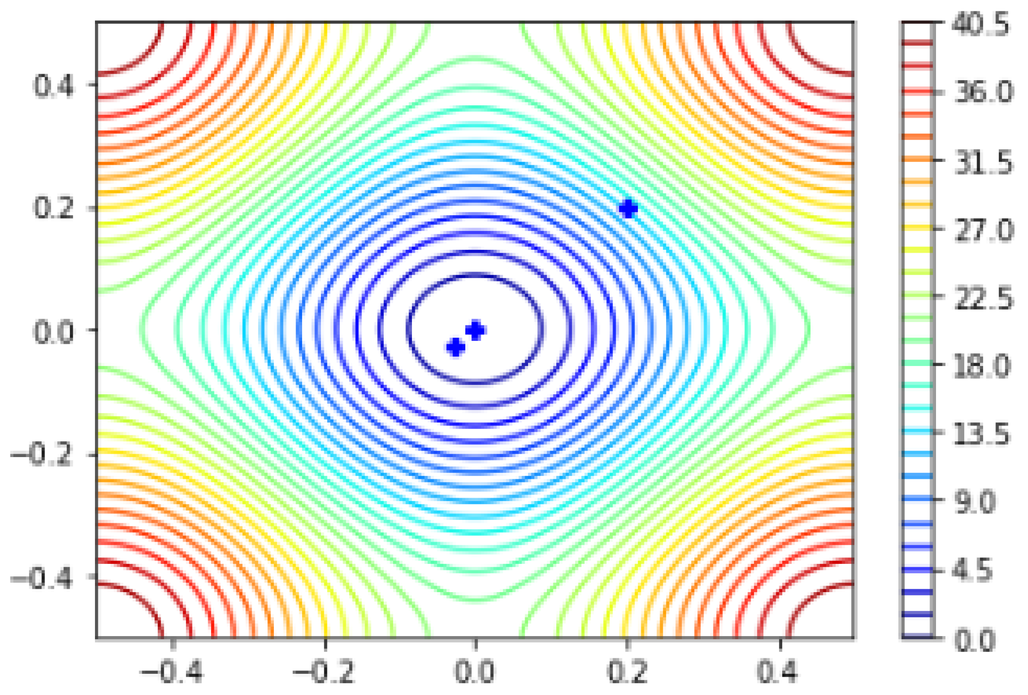
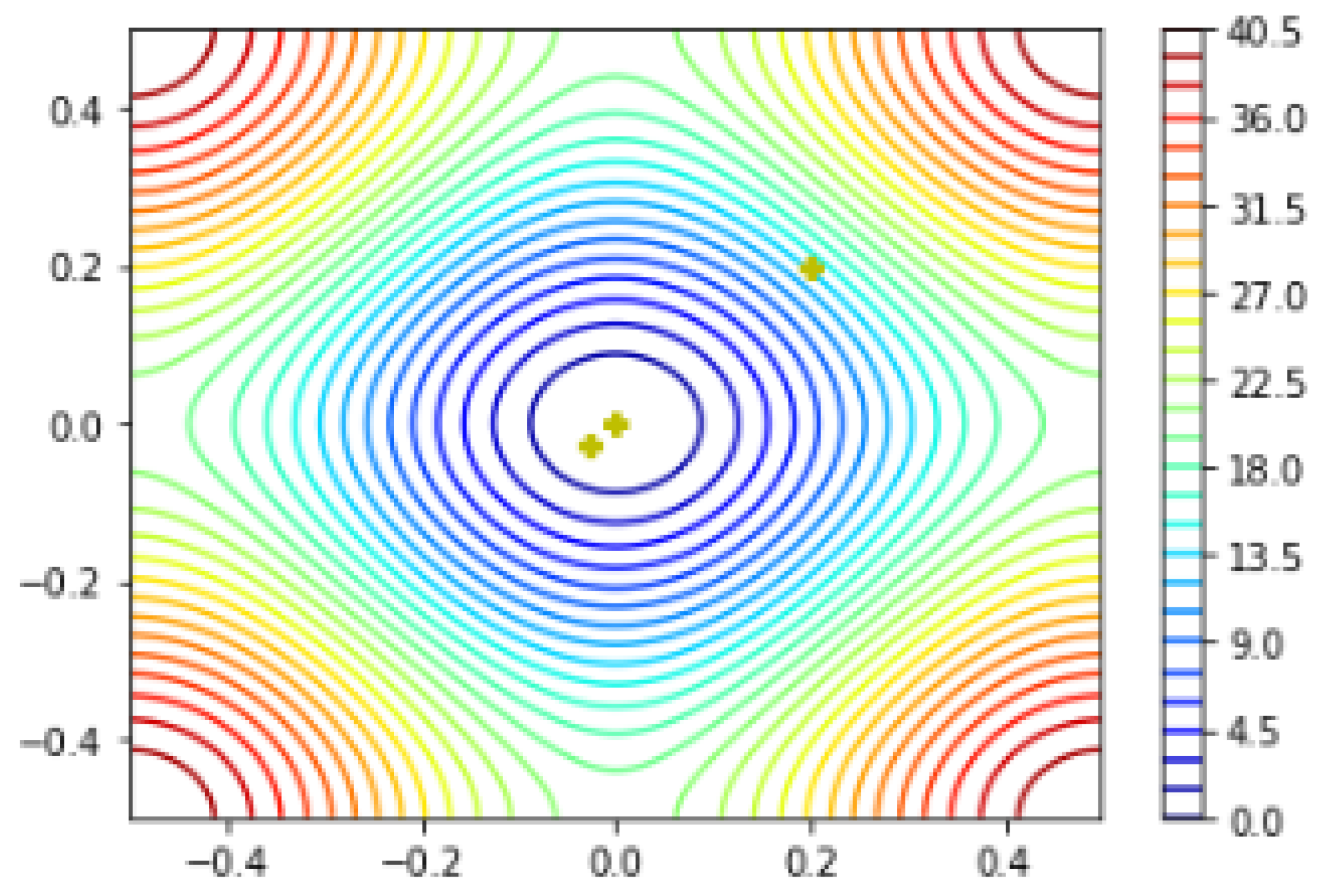
Example 3.

Consider the non-convex Rastrigin function f such that

$$f\left(x\right)=10d+\sum _{i=1}^d[x_i^2-10cos\left(2\pi x_i\right)]$$

Following Figure 8 represents the surface plot of the Rastrigin function:

Figure 8. Surface plot of the Rastrigin function.

The Rastrigin function f has a global minimum at

$$x^{*}=(0,0,\dots ,0),$$

with value

$$f\left(x^{*}\right)=0.$$

We tested modified q-BFGS, q-BFGS, and, BFGS algorithms for initial point $x^0=(0.2,0.2)$.

The global minima and plotting points of the Rastrigin function using the modified q-BFGS algorithm can be observed in Figure 9.

Figure 9. Global minima of the Rastrigin function using the modified q-BFGS algorithm.

The numerical results for the Rastrigin function, using the modified q-BFGS algorithm are as follows:

For the starting point $x^0=(0.2,0.2),$ the Rastrigin function converges to

$$\begin{array}{cc}\hfill & x^{*}={[-6.83810097023008e^{-6},-6.83810097023008e^{-6}]}^T,\hfill \\ & \mathrm{with}\hfill \\ & f\left(x^{*}\right)=1.85534789132191e^{-9}\mathrm{and}{\nabla }_{q}f\left(x^{*}\right)={[-1.3676e^{-6},-1.3676e^{-6}]}^T.\hfill \end{array}$$

NI/NF/NG = $4/18/6$.

The global minima and plotting points of the Rastrigin function using the q-BFGS algorithm can be observed in Figure 10.

Figure 10. Global minima of the Rastrigin function using q-BFGS algorithm.

The numerical results for the Rastrigin function, using the q-BFGS algorithm are as follows:

For the starting point $x^0=(0.2,0.2),$ The Rastrigin function converges to

$$\begin{array}{cc}\hfill & x^{*}={[-1.18906228e^{-06},-2.65293229e^{-07}]}^T,\hfill \\ & \mathrm{with}\hfill \\ & f\left(x^{*}\right)=2.944648969105401e^{-10}\mathrm{and}{\nabla }_{q}f\left(x^{*}\right)={[0.,0.]}^T.\hfill \end{array}$$

NI/NF/NG = $5/24/8$.

The global minima and plotting points of the Rastrigin function using the BFGS algorithm can be observed in Figure 11.

Figure 11. Global minima of the Rastrigin function using BFGS algorithm.

The numerical results for the Rastrigin function using the BFGS algorithm are as follows:

For the starting point $x^0=(0.2,0.2),$ the Rastrigin function converges to

$$\begin{array}{cc}\hfill & x^{*}={(-7.14289963e^{-09},-7.37267609e^{-09})}^T,\hfill \\ & \mathrm{with}\hfill \\ & f\left(x^{*}\right)=2.1316282072803006e^{-14}\mathrm{and}\nabla f\left(x^{*}\right)={(1.1920929e^{-07},0.0000000e^{00})}^T.\hfill \end{array}$$

NI/NF/NG = $7/36/12$.

From the above numerical results, we conclude that using the modified q-BFGS algorithm, we can reach the critical point by taking the least number of iterations.

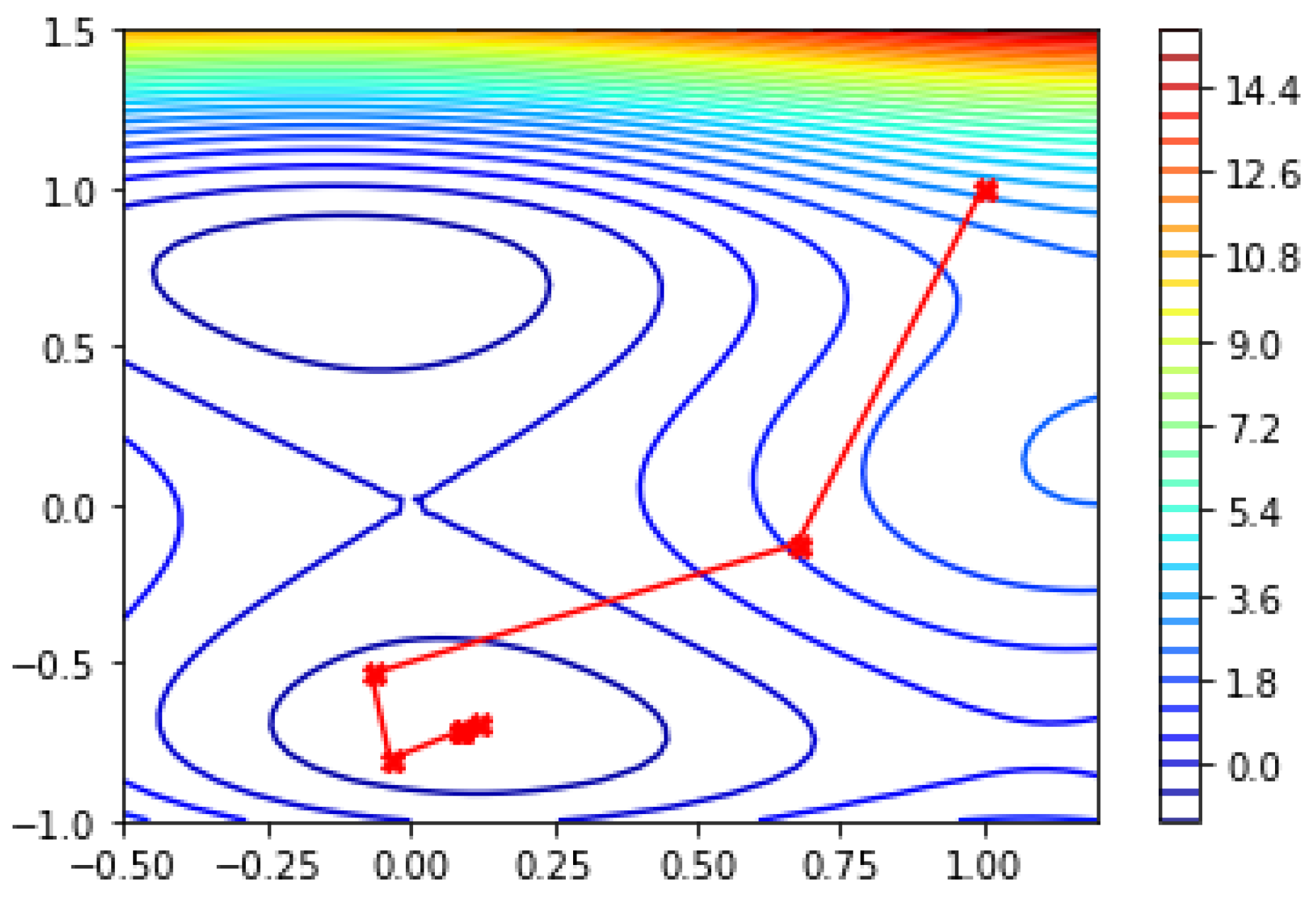
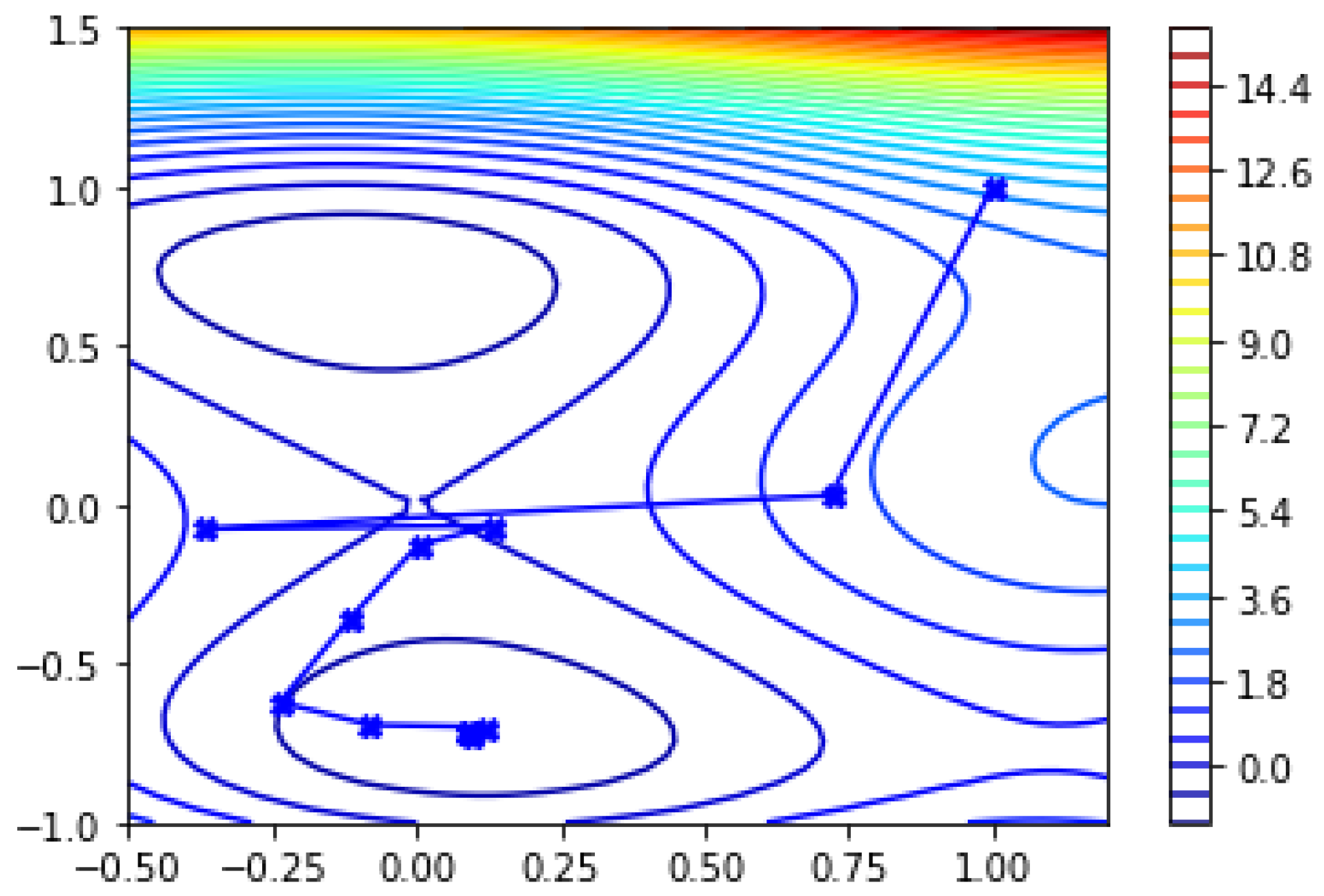
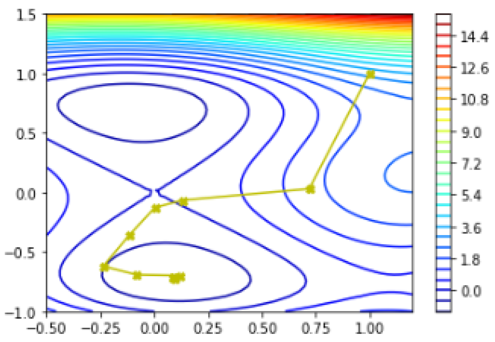
Example 4.

Consider the SIX-HUMP CAMEL function $f:$${\mathbb{R}}^2\to \mathbb{R}$ such that

$$f\left(x\right)=\left(4-2.1x_1^2+\frac{x_1^4}{3}\right)x_1^2+x_1{x}_2+(-4+4x_2^2)x_2^2$$

The Figure 12 on the left shows the SIX-HUMP CAMEL function on its recommended input domain and on the right shows only a portion of this domain for easier view of the function’s key characteristics. The function f has six local minima, two of which are global.

Figure 12. Surface plot of the SIX-HUMP CAMEL function.

Input Domain: The function is usually evaluated on the rectangle $x_1\in [-3,3],x_2\in [-2,2].$

This function has a global minimum at

$$x^{*}=(0.0898,-0.7126)\mathrm{and}(-0.0898,0.7126),$$

with value

$$f\left(x^{*}\right)=-1.0316.$$

For the starting point $x^0=(1,1),$ with the modified q-BFGS algorithm f converges to $x^{*}$ in eight iterations whereas with q-BFGS and BFGS it takes 13 iterations. Table 2, Table 3, and Table 4 give numerical results and Figure 13, Figure 14, and Figure 15 represents the global minima and sequence of iterative points generated with modified q-BFGS, q-BFGS and BFGS algorithms, respectively.

Table 2. Numerical results for Modified q-BFGS algorithm.

S.N.	x	$\mathit{f}\left(\mathit{x}\right)$	${\mathit{\nabla }}_{\mathit{q}}\mathit{f}\left(\mathit{x}\right)$
1	${(1,1)}^T$	3.23333333333333	${(2.59999999,8.9999998)}^T$
2	${(0.675,-0.12499997)}^T$	1.27218227259399	${(2.97185835,1.64374981)}^T$
3	${(-0.06796459,-0.53593743)}^T$	−0.764057148938559	${(-1.0770199,1.75654714)}^T$
4	${(-0.0353348602,-0.8064736058)}^T$	−0.876032180235736	${(-1.08878201,-1.97602868)}^T$
5	${(0.117691114989,-0.69297924267)}^T$	−1.02498975962408	${(0.23490147,0.33700269)}^T$
6	${(0.087916835437,-0.709453427634)}^T$	−1.03153652682667	${(-0.01181639,0.05018343)}^T$
7	${(0.089782273326,-0.71271422021)}^T$	−1.03162840874522	${(-0.00052364,-0.00100674)}^T$
8	${(0.089842117966,-0.71265601378)}^T$	−1.03162845348855	${(1.20226364\times {10}^{-6},6.54303983\times {10}^{-6})}^T$

Table 2. Numerical results for Modified q-BFGS algorithm.

S.N.	x	$\mathit{f}\left(\mathit{x}\right)$	${\mathit{\nabla }}_{\mathit{q}}\mathit{f}\left(\mathit{x}\right)$
1	${(1,1)}^T$	3.23333333333333	${(2.59999999,8.9999998)}^T$
2	${(0.675,-0.12499997)}^T$	1.27218227259399	${(2.97185835,1.64374981)}^T$
3	${(-0.06796459,-0.53593743)}^T$	−0.764057148938559	${(-1.0770199,1.75654714)}^T$
4	${(-0.0353348602,-0.8064736058)}^T$	−0.876032180235736	${(-1.08878201,-1.97602868)}^T$
5	${(0.117691114989,-0.69297924267)}^T$	−1.02498975962408	${(0.23490147,0.33700269)}^T$
6	${(0.087916835437,-0.709453427634)}^T$	−1.03153652682667	${(-0.01181639,0.05018343)}^T$
7	${(0.089782273326,-0.71271422021)}^T$	−1.03162840874522	${(-0.00052364,-0.00100674)}^T$
8	${(0.089842117966,-0.71265601378)}^T$	−1.03162845348855	${(1.20226364\times {10}^{-6},6.54303983\times {10}^{-6})}^T$

Here, we obtain $x^{*}={(0.089842117966,-0.71265601378)}^T$

$$f\left(x^{*}\right)=-1.03162845348988\mathrm{and}{\nabla }_{q}f\left(x^{*}\right)={(-6.20473783\times {10}^{-09},0.00000000\times {10}^{+00})}^T$$

Figure 13. Global minima of SIX-HUMP CAMEL function using modified q-BFGS algorithm.

Table 3. Numerical results for q-BFGS algorithm [34].

S.N.	x	$\mathit{f}\left(\mathit{x}\right)$	${\mathit{\nabla }}_{\mathit{q}}\mathit{f}\left(\mathit{x}\right)$
1	${(1,1)}^T$	3.23333333333333	${(2.59999999,8.9999998)}^T$
2	${(0.71968495,0.02967868)}^T$	1.57257718494530	${(3.04212661,0.4826738)}^T$
3	${(-0.36642555,-0.07524058)}^T$	0.505072874807150	${(-2.60658417,0.22868392)}^T$
4	${(0.13008033,-0.06568514)}^T$	0.0413558838831559	${(0.95654292,0.65102699)}^T$
5	${(0.00245036,-0.12816569)}^T$	−0.0649165012454617	${(-0.10856293,0.99409097)}^T$
6	${(-0.11507302,-0.35694646)}^T$	−0.351034437749229	${(-1.26477125,2.01283747)}^T$
7	${(-0.23737914,-0.62081297)}^T$	−0.581320173229039	${(-2.40899478,0.90085665)}^T$
8	${(-0.08148802,-0.6924283)}^T$	−0.915418626192531	${(-1.33979439,0.14610549)}^T$
9	${(0.11917819,-0.6987523)}^T$	−1.02633316281778	${(0.24050227,0.25049034)}^T$
10	${(0.0912121,-0.72252832)}^T$	−1.03082558867975	${(0.00080671,-0.16366308)}^T$
11	${(0.087625,-0.71111103)}^T$	−1.03159319420704	${(-0.01575222,0.02301181)}^T$
12	${(0.09005303,-0.71260578)}^T$	−1.03162824822151	${(0.00169591,0.00104015)}^T$
13	${(0.08983369,-0.71266332)}^T$	−1.03162845277086	${(-7.18180083\times {10}^{-5},-1.21481195\times {10}^{-4})}^T$

Table 3. Numerical results for q-BFGS algorithm [34].

S.N.	x	$\mathit{f}\left(\mathit{x}\right)$	${\mathit{\nabla }}_{\mathit{q}}\mathit{f}\left(\mathit{x}\right)$
1	${(1,1)}^T$	3.23333333333333	${(2.59999999,8.9999998)}^T$
2	${(0.71968495,0.02967868)}^T$	1.57257718494530	${(3.04212661,0.4826738)}^T$
3	${(-0.36642555,-0.07524058)}^T$	0.505072874807150	${(-2.60658417,0.22868392)}^T$
4	${(0.13008033,-0.06568514)}^T$	0.0413558838831559	${(0.95654292,0.65102699)}^T$
5	${(0.00245036,-0.12816569)}^T$	−0.0649165012454617	${(-0.10856293,0.99409097)}^T$
6	${(-0.11507302,-0.35694646)}^T$	−0.351034437749229	${(-1.26477125,2.01283747)}^T$
7	${(-0.23737914,-0.62081297)}^T$	−0.581320173229039	${(-2.40899478,0.90085665)}^T$
8	${(-0.08148802,-0.6924283)}^T$	−0.915418626192531	${(-1.33979439,0.14610549)}^T$
9	${(0.11917819,-0.6987523)}^T$	−1.02633316281778	${(0.24050227,0.25049034)}^T$
10	${(0.0912121,-0.72252832)}^T$	−1.03082558867975	${(0.00080671,-0.16366308)}^T$
11	${(0.087625,-0.71111103)}^T$	−1.03159319420704	${(-0.01575222,0.02301181)}^T$
12	${(0.09005303,-0.71260578)}^T$	−1.03162824822151	${(0.00169591,0.00104015)}^T$
13	${(0.08983369,-0.71266332)}^T$	−1.03162845277086	${(-7.18180083\times {10}^{-5},-1.21481195\times {10}^{-4})}^T$

Here, we obtain $x^{*}={(0.08983369,-0.71266332)}^T,$

$$f\left(x^{*}\right)=-1.0316284534898477\mathrm{and}{\nabla }_{q}f\left(x^{*}\right)={(-0.00000000\times {10}^{+00},9.65876859\times {10}^{-07})}^T.$$

Using this q-BFGS algorithm, we can reach the critical point by taking 13 iterations.

Figure 14. Global minima of SIX-HUMP CAMEL function using q-BFGS algorithm.

Table 4. Numerical results for BFGS algorithm.

S.N.	x	$\mathit{f}\left(\mathit{x}\right)$	${\mathit{\nabla }}_{\mathit{q}}\mathit{f}\left(\mathit{x}\right)$
1	${(1,1)}^T$	3.23333333333333	${(2.59999999,8.9999998)}^T$
2	${(0.71968497,0.02967869)}^T$	1.5725772653791203	${(3.04212611,0.48267368)}^T$
3	${(0.13008034,-0.06568512)}^T$	0.041355907444434827	${(0.95654306,0.65102689)}^T$
4	${(0.00245035,-0.12816566)}^T$	−0.06491646830150141	${(-0.10856298,0.99409077)}^T$
5	${(-0.11507301,-0.35694647)}^T$	−0.35103445558228663	${(-1.26477118,2.01283762)}^T$
6	${(-0.23737911,-0.62081301)}^T$	−0.5813202779118049	${(-2.40899456,0.90085617)}^T$
7	${(-0.08148803,-0.6924282)}^T$	−0.9154186025665918	${(-1.33979439,0.1461069)}^T$
8	${(0.11917811,-0.69875236)}^T$	−1.0263331977999757	${(0.24050162,0.25048941)}^T$
9	${(0.09121207,-0.72252828)}^T$	−1.0308255945761227	${(0.00080669,-0.16366242)}^T$
10	${(0.08762501,-0.71111104)}^T$	−1.031593194593363	${(-0.01575207,0.02301181)}^T$
11	${(0.09005304,-0.71260578)}^T$	−1.031628248214576	${(0.00169598,0.00104006)}^T$
12	${(0.08983368,-0.7126633)}^T$	−1.0316284527721356	${(0.000016959,0.000104006)}^T$
13	${(0.08984197,-0.71265633)}^T$	−1.0316284534898297	${(-7.19424520\times {10}^{-5},-1.21236354\times {10}^{-4})}^T$

Table 4. Numerical results for BFGS algorithm.

S.N.	x	$\mathit{f}\left(\mathit{x}\right)$	${\mathit{\nabla }}_{\mathit{q}}\mathit{f}\left(\mathit{x}\right)$
1	${(1,1)}^T$	3.23333333333333	${(2.59999999,8.9999998)}^T$
2	${(0.71968497,0.02967869)}^T$	1.5725772653791203	${(3.04212611,0.48267368)}^T$
3	${(0.13008034,-0.06568512)}^T$	0.041355907444434827	${(0.95654306,0.65102689)}^T$
4	${(0.00245035,-0.12816566)}^T$	−0.06491646830150141	${(-0.10856298,0.99409077)}^T$
5	${(-0.11507301,-0.35694647)}^T$	−0.35103445558228663	${(-1.26477118,2.01283762)}^T$
6	${(-0.23737911,-0.62081301)}^T$	−0.5813202779118049	${(-2.40899456,0.90085617)}^T$
7	${(-0.08148803,-0.6924282)}^T$	−0.9154186025665918	${(-1.33979439,0.1461069)}^T$
8	${(0.11917811,-0.69875236)}^T$	−1.0263331977999757	${(0.24050162,0.25048941)}^T$
9	${(0.09121207,-0.72252828)}^T$	−1.0308255945761227	${(0.00080669,-0.16366242)}^T$
10	${(0.08762501,-0.71111104)}^T$	−1.031593194593363	${(-0.01575207,0.02301181)}^T$
11	${(0.09005304,-0.71260578)}^T$	−1.031628248214576	${(0.00169598,0.00104006)}^T$
12	${(0.08983368,-0.7126633)}^T$	−1.0316284527721356	${(0.000016959,0.000104006)}^T$
13	${(0.08984197,-0.71265633)}^T$	−1.0316284534898297	${(-7.19424520\times {10}^{-5},-1.21236354\times {10}^{-4})}^T$

Here, we obtain $x^{*}={(0.08984197,-0.71265633)}^T,$

$$f\left(x^{*}\right)=-1.0316284534898448\mathrm{and}\nabla f\left(x^{*}\right)={(-2.68220901\times {10}^{-07},9.98377800\times {10}^{-07})}^T.$$

Using this BFGS algorithm, we can reach the critical point by taking 13 iterations.

Figure 15. Global minima of SIX-HUMP CAMEL function using BFGS algorithm.

We conclude that using the modified q-BFGS algorithm, we can reach the critical point by taking the least number of iterations. From the performance results and plotting points for the multimodal functions it could be seen that the q-descent direction has a mechanism to escape from many local minima and move towards the global minimum.

Now, we compare the performance of numerical algorithms for large dimensional Rosenbrock and Wood function. Numerical results for these functions are given in Table 5 and Table 6.

Numerical results for the large dimensional Rosenbrock function for${\mathbf{x}}^{\mathbf{0}}=(\mathbf{0},\mathbf{0},\dots ,\mathbf{0})$

$$\begin{array}{c}\hfill f\left(x\right)=\sum _{i=1}^{d-1}[100{(x_{i+1}-{x_i}^2)}^2+{(x_i-1)}^2]\end{array}$$

Table 5. Comparison of numerical results of Modified q-BFGS, q-BFGS, and BFGS algorithm for the large dimensional Rosenbrock function.

S.No.	Dimension	Modified q-BFGS	q-BFGS	BFGS
		NI/NF/NG	NI/NF/NG	NI/NF/NG
1	10	58/889/132	63/972/81	61/1365/123
2	50	242/15,432/300	253/17,316/324	253/17,199/337
3	100	466/63,088/604	486/64,056/636	479/64,741/641
4	200	904/209,912/1175	978/248,056/1228	956/253,674/1262

Table 5. Comparison of numerical results of Modified q-BFGS, q-BFGS, and BFGS algorithm for the large dimensional Rosenbrock function.

S.No.	Dimension	Modified q-BFGS	q-BFGS	BFGS
		NI/NF/NG	NI/NF/NG	NI/NF/NG
1	10	58/889/132	63/972/81	61/1365/123
2	50	242/15,432/300	253/17,316/324	253/17,199/337
3	100	466/63,088/604	486/64,056/636	479/64,741/641
4	200	904/209,912/1175	978/248,056/1228	956/253,674/1262

Numerical results for large dimensional WOOD function [39] for${\mathbf{x}}^{\mathbf{0}}=(\mathbf{0},\mathbf{0},\dots ,\mathbf{0})$

Table 6. Comparison of numerical results of Modified q-BFGS, q-BFGS, and BFGS algorithm for Large Dimensional Wood function.

S.No.	Dimension	Modified q-BFGS	q-BFGS	BFGS
		NI/NF/NG	NI/NF/NG	NI/NF/NG
1	20	85/1976/98	91/2872/130	103/2478/118
2	80	162/19,745/198	193/21,250/259	209/22,366/276
3	100	197/19,965/255	240/30,714/301	254/29,290/290
4	200	296/75,686/397	370/93,538/463	378/93,678/466

Table 6. Comparison of numerical results of Modified q-BFGS, q-BFGS, and BFGS algorithm for Large Dimensional Wood function.

S.No.	Dimension	Modified q-BFGS	q-BFGS	BFGS
		NI/NF/NG	NI/NF/NG	NI/NF/NG
1	20	85/1976/98	91/2872/130	103/2478/118
2	80	162/19,745/198	193/21,250/259	209/22,366/276
3	100	197/19,965/255	240/30,714/301	254/29,290/290
4	200	296/75,686/397	370/93,538/463	378/93,678/466

We have taken 20 test problems to show the proposed method’s efficiency and numerical results. We take tolerance $ϵ={10}^{-6},{\sigma }_1=0.0001,\mathrm{and}{\sigma }_2=0.9$. Our numerical results are shown in Table 7, Table 8 and Table 9 with the problem number(S.N.), problem name, Dimension (DIM), starting point, the total number of iterations (NI), the total number of function evaluations (NF), the total number of gradient evaluations (NG), respectively.

Table 7. Numerical results for Modified q-BFGS algorithm.

S.N.	Problems	${\mathit{x}}^0$	DIM	NI	NF	NG	${\mathit{x}}^{*}$
1	ROSENBROCK	${(-1.5,-1)}^T$	2	25	95	47	${(1.0000,1.0000)}^T$
2	FROTH	${(0.5,-2)}^T$	2	9	37	20	${(11.4128,-0.8968)}^T$
3	BADSCP	${(0,1)}^T$	2	174	618	272	${(1.0981\times {10}^{-5},9.1062)}^T$
4	BADSCB	${(1,1)}^T$	2	11	100	80	${(1000000.0000,1.9999\times {10}^{-6})}^T$
5	BEALE	${(3,1)}^T$	2	12	44	21	${(3.0000,0.5000)}^T$
6	JENSAM	${(1,0.4)}^T$	2	15	57	20	${(0.56094,0.56094)}^T$
7	WOOD	${(-3,-1,-3,-1)}^T$	4	42	205	52	${(1.0000,1.0000,1.0000,1.0000)}^T$
8	POWELL SINGULAR	${(3,-1,0,1)}^T$	4	23	91	46	${(-0.0011,0.0001,0.0009,0.0009)}^T$
9	RASTRIGIN	${(0.2,0.2)}^T$	2	4	18	6	${(-6.8381\times {10}^{-5},-6.8381\times {10}^{-5})}^T$
10	GOLDSTEIN PRICE	${(0.5,0.5)}^T$	2	12	106	84	${(5.4911\times {10}^{-5},-1.0000)}^T$
11	THREE-HUMP CAMEL	${(-2.5,0)}^T$	2	5	19	10	${(8.3463\times {10}^{-8},1.9707\times {10}^{-7})}^T$
12	COLVILLE	${(0,0,0,0)}^T$	4	27	109	56	${(1.0000,1.0000,1.0000,1.0000)}^T$
13	BOOTH	${(2,2)}^T$	2	2	11	8	${(1.0000,3.0000)}^T$
14	SINE VALLEY	${(3\pi /2,-1)}^T$	2	35	115	46	${(-1.4495\times {10}^{-11},-1.6686\times {10}^{-11})}^T$
15	BRANIN	${(9.3,3)}^T$	2	5	18	9	${(9.4248,2.4750)}^T$
16	SIX HUMP CAMEL	${(1,1)}^T$	2	8	32	17	${(0.0898,-0.7126)}^T$
17	HIMMELBLAU	${(1,1)}^T$	2	9	37	20	${(3.0000,2.0000)}^T$
18	SHEKEL	${(0,0,0,0)}^T$	4	14	105	35	${(4.0007,4.0005,3.9997,3.9995)}^T$
19	HARTMAN 3D	${(0,0.5,0.4)}^T$	3	10	100	21	${(0.1146,0.5556,0.8525)}^T$
20	GRIEWANK	${(2,-1.2)}^T$	2	8	25	9	${(-6.9305\times {10}^{-5},-5.0749\times {10}^{-5})}^T$

Table 8. Numerical results for q-BFGS algorithm.

S.N.	Problems	${\mathit{x}}^0$	DIM	NI	NF	NG	${\mathit{x}}^{*}$
1	ROSENBROCK	${(-1.5,-1)}^T$	2	47	198	66	$(1.0000,1.{0000}^T$
2	FROTH	${(0.5,-2)}^T$	2	9	30	10	${(11.4127,-0.8968)}^T$
3	BADSCP	${(0,1)}^T$	2	158	609	203	${(1.0981\times {10}^{-5},9.1061)}^T$
4	BADSCB	${(1,1)}^T$	2	-	-	-	-
5	BEALE	${(3,1)}^T$	2	13	48	16	${(3.0000,0.5000)}^T$
6	JENSAM	${(1,0.4)}^T$	2	17	66	22	${(0.56095,0.56095)}^T$
7	WOOD	${(-3,-1,-3,-1)}^T$	4	87	309	103	${(1.0000,1.0000,1.0000,1.0000)}^T$
8	POWELL SINGULAR	${(3,-1,0,1)}^T$	4	37	126	42	$(2.3008\times {10}^{-4},-2.3007\times {10}^{-5},$$9.0539\times {10}^{-4},9.0545\times {10}^{-4}{)}^T$
9	RASTRIGIN	${(0.2,0.2)}^T$	2	5	24	8	${(-1.1890\times {10}^{-6},-2.6529\times {10}^{-7})}^T$
10	GOLDSTEIN PRICE	${(0.5,0.5)}^T$	2	-	-	-	-
11	THREE-HUMP CAMEL	${(-2.5,0)}^T$	2	8	36	12	${(-1.7475,0.8738)}^T$
12	COLVILLE	${(0,0,0,0)}^T$	4	26	102	34	${(1.0000,1.0000,1.0000,1.0000)}^T$
13	BOOTH	${(2,2)}^T$	2	3	15	5	${(1.0000,3.0000)}^T$
14	SINE VALLEY	${(3\pi /2,-1)}^T$	2	37	132	44	${(4.0788\times {10}^{-10},4.262\times {10}^{-10})}^T$
15	BRANIN	${(9.3,3)}^T$	2	6	24	8	${(9.4248,2.4750)}^T$
16	SIX HUMP CAMEL	${(1,1)}^T$	2	13	54	18	${(0.0898,-0.7126)}^T$
17	HIMMELBLAU	${(1,1)}^T$	2	8	39	13	${(3.0000,2.0000)}^T$
18	SHEKEL	${(0,0,0,0)}^T$	4	14	105	35	${(4.0007,4.0006,3.9997,3.9995)}^T$
19	HARTMAN 3D	${(0,0.5,0.4)}^T$	3	11	63	21	${(0.1088,0.5556,0.8526)}^T$
20	GRIEWANK	${(2,-1.2)}^T$	2	8	27	9	${(8.4001\times {10}^{-5},3.1323\times {10}^{-4})}^T$

Table 9. Numerical results for BFGS algorithm.

S.N.	Problems	${\mathit{x}}^0$	DIM	NI	NF	NG	${\mathit{x}}^{*}$
1	ROSENBROCK	${(-1.5,-1)}^T$	2	49	213	71	$(1.0000,1.{0000}^T$
2	FROTH	${(0.5,-2)}^T$	2	9	30	10	${(11.4128,-0.8968)}^T$
3	BADSCP	${(0,1)}^T$	2	-	-	-	-
4	BADSCB	${(1,1)}^T$	2	-	-	-	-
5	BEALE	${(3,1)}^T$	2	13	48	16	${(3.0000,0.5000)}^T$
6	JENSAM	${(1,0.4)}^T$	2	17	66	22	${(0.56095,0.56095)}^T$
7	WOOD	${(-3,-1,-3,-1)}^T$	4	89	525	105	${(1.0000,1.0000,1.0000,1.0000)}^T$
8	POWELL SINGULAR	${(3,-1,0,1)}^T$	4	41	230	46	$(7.759\times {10}^{-4},-7.7607\times {10}^{-5},$$-7.5812\times {10}^{-4},-7.581\times {10}^{-4}{)}^T$
9	RASTRIGIN	${(0.2,0.2)}^T$	2	7	36	12	${(-7.1429\times {10}^{-9},-7.3727\times {10}^{-7})}^T$
10	GOLDSTEIN PRICE	${(0.5,0.5)}^T$	2	17	75	25	${(-9.9828\times {10}^{-9},-1.0000)}^T$
11	THREE-HUMP CAMEL	${(-2.5,0)}^T$	2	8	36	12	${(-1.7475,0.8738)}^T$
12	COLVILLE	${(0,0,0,0)}^T$	4	31	190	38	${(1.0000,1.0000,1.0000,1.0000)}^T$
13	BOOTH	${(2,2)}^T$	2	3	15	5	${(1.0000,3.0000)}^T$
14	SINE VALLEY	${(3\pi /2,-1)}^T$	2	37	141	47	${(-5.9619\times {10}^{-6},-5.9674\times {10}^{-6})}^T$
15	BRANIN	${(9.3,3)}^T$	2	6	24	8	${(9.4248,2.4750)}^T$
16	SIX HUMP CAMEL	${(1,1)}^T$	2	13	54	18	${(0.0898,-0.7126)}^T$
17	HIMMELBLAU	${(1,1)}^T$	2	8	39	13	${(3.0000,2.0000)}^T$
18	SHEKEL	${(0,0,0,0)}^T$	4	12	160	32	${(4.0007,4.0006,3.9997,3.9995)}^T$
19	HARTMAN 3D	${(0,0.5,0.4)}^T$	3	14	80	20	${(0.1146,0.5556,0.8525)}^T$
20	GRIEWANK	${(2,-1.2)}^T$	2	10	33	11	${(6.872\times {10}^{-8},-7.2441\times {10}^{-4})}^T$

Table 5, Table 6, Table 7, Table 8 and Table 9 show that the modified q-BFGS algorithm solves about 86% of the test problems with the least number of iterations, 82% of the test problems with the least number of function evaluations, and 52% of the test problems with the least number of gradient evaluations. Therefore, with Figure 16, Figure 17 and Figure 18 we conclude that the modified q-BFGS performs better than other algorithms and improves the performance in fewer iterations, function evaluations, and gradient evaluations.

Figure 16. Performance Profile based on number of iterations.

Figure 17. Performance Profile based on number of function evaluations.

Figure 18. Performance Profile based on number of gradient evaluations.

In Figure 17 and Figure 18 the graph of q-BFGS and BFGS method does not converge to 1 as the methods fail to minimize two problems for each as given in Table 8 and Table 9.

6. Conclusions and Future Directions

We have given a new q-quasi-Newton equation and proposed a modified q-BFGS method for unconstrained minimization based on this new q-quasi-Newton equation. The method converges globally with a q-gradient-based Armijo–Wolfe line search. The q-gradient allows the search direction to be taken from a diverse set of directions and takes large steps to converge. From the performance results and plotting points for the multimodal functions, it could be seen that the q-descent direction and q-gradient-based line search have a mechanism to escape from many local minima and move towards the global minimum. The first order q-differentiability of the function is sufficient to prove the global convergence of the proposed method. The convergence and numerical results show that the algorithm given in this paper is very successful. However, many other q-quasi-Newton methods still need to be studied using the q-derivative.