Market Volatility Spillover, Network Diffusion, and Financial Systemic Risk Management: Financial Modeling and Empirical Study

Abstract

With the accelerated pace of financial globalization and the gradual increase in linkages among financial markets, correctly identifying and describing the risk spillover and network diffusion in the financial system is extremely important for the prevention and management of systemic risk. Based on this, this paper takes the equity markets of 17 countries around the world from 2007 to 2022 as the research object, measures the volatility spillover effect of global financial markets using R-Vine Copula and the DY spillover index, constructs the volatility spillover network of global financial markets, discovers the spillover and diffusion pattern of global financial market risks, and provides relevant suggestions for systemic risk management. It is found that (1) there are certain aggregation characteristics in the network diffusion of global financial market volatility spillover; (2) developed European countries such as the Netherlands, France, the UK, and Germany are at the center of the network and have a strong influence; (3) Asian countries such as China, Japan, and India are at the periphery of the network; and (4) shocks from crisis events enhance the global financial market volatility spillover effect. Based on the above findings, effective prevention of global financial market risk volatility spillover and network diffusion and reduction in systemic risk need to be carried out in two ways. First, by focusing on the financial markets of key countries in the network, such as the Netherlands, the UK, France, and Germany. The second approach is to mitigate the uneven development in global financial markets and reduce the high correlation among them.

1. Introduction

In recent years, as financial globalization has continued to deepen, the linkages among financial markets have gradually strengthened. Furthermore, different markets have factors, such as market structures, trading systems, and investment environments, that differ to some extent. Moreover, with the accelerated pace of information modernization, the transmission of information between markets has become more complex and faster. If this information transmission is not properly managed, it may trigger financial risks and result in incalculable consequences for markets [1,2]. For example, the U.S. subprime mortgage crisis in 2007 triggered the international financial crisis, the European debt crisis in 2011 led to a sharp decline in global financial markets, and the COVID-19 epidemic in 2020 triggered global capital market shocks. Therefore, it is of significant importance to set up risk warning mechanisms, and systemic risks can be managed if we can accurately characterize this information transmission and describe the correlation of information between markets.

To study this information correlation between markets, an increasing number of scholars use the term “spillover effect” to describe the interaction between markets [3,4,5]. Typically, the risk spillover effect refers to the exchange of information between markets, such that if one market changes in a certain way, other markets will also be affected, and at the same time, this effect will continue to be transmitted, causing changes across all markets [6,7]. At the same time, financial globalization has led to closer economic ties and increasing openness between different countries and regions, and while improving the efficiency of market transactions, risk spillover effects are also interacting across sectors. Risks in a single financial market can spillover to other market systems through open channels, triggering the contagion and spread of financial risks, which can lead to systemic risks and financial crises and affect the entire financial system. Therefore, correctly identifying and characterizing risk spillovers and network diffusion in the financial system is extremely important to prevent and manage systemic risks.

As a barometer of socio-economic development, equity market fluctuations are extremely important. In addition, against the background of deepening global financial liberalization and integration, cross-border capital flows are becoming more frequent and equity markets are becoming more closely linked, gradually forming a network of risk correlations that “move the whole body by one hair”. Therefore, accurate measurement of global equity market systemic risk levels, understanding of risk formation rules and transmission mechanisms, and accurate identification of risk prevention difficulties are of reference value for national economies to improve systemic risk warning and prevention systems.

Based on this, this paper measures the volatility spillover effects of global financial markets and constructs a volatility spillover network, aiming to identify the spillover and diffusion patterns of global financial market risks and provide relevant suggestions for systemic risk management. The paper is organized as follows: The second section briefly reviews the related literature; the third section introduces the relevant methods for volatility spillover measurement and network diffusion quantification; the fourth section presents an empirical study, which mainly includes volatility spillover measurement and network diffusion analysis; finally, the conclusion provides relevant suggestions for systemic risk management in global financial markets based on the research findings.

2. Literature Review

In the financial system, there is often a certain degree of correlation between different markets and different assets, and the occurrence of risk causes volatility spillover effects between markets. Therefore, the study of correlation is particularly important for analyzing volatility spillover effects between markets. Currently, the main volatility spillover measures are developed based on the correlation between variables, including Granger causality tests, VAR models, CoVaR models, GARCH cluster models, MSV, and MVMQ-CAViaR [8,9,10,11]. Among these, Granger causality tests and VAR models are widely used in risk spillover measures of markets [12,13]. VAR models are often used to test causality between market volatility because they can better solve the problem of endogeneity and heteroskedasticity of variables. However, the inability to perform dynamic correlation measures is a shortcoming of VAR models, and CoVaR models can better compensate for this shortcoming and are widely used in measuring the intensity and direction of risk spillovers [14]. Similarly, GARCH cluster models are also used to solve the risk volatility spillover problem, and the empirical results show that GARCH cluster models can better characterize the heteroskedasticity of the residual terms of the return series [15,16]. GARCH cluster models have been improved and extended in practice, such as GARCH-M, APGARCH, NAGARCH, TGARCH, and EGARCH [17,18,19]. Since financial risk spillovers involve multiple variables, multivariate GARCH cluster models such as VECH-GARCH, CCC-GARCH, BEKK-GARCH, and DCC-GARCH are also widely used for the measurement of volatility spillovers [20,21,22,23]. These models can measure both univariate spillover characteristics and portray multivariate spillover relationships.

However, it is worth noting that the correlation between financial markets is often nonlinear, meaning that the risk spillover is not in linear manner [24]. Using the above approach requires satisfying the assumption of multivariate normal distribution, a premise that is too stringent for characterizing complex financial market dependencies. Copula functions are increasingly used in the study of volatility spillovers in financial markets because they can effectively capture nonlinear dependencies between markets [25,26,27,28]. In the description of multivariate spillover relationships, the traditional binary Copula method faces the problem of “dimensional catastrophe”, and the multivariate Copula method lacks accuracy and flexibility [29]. The Vine Copula approach can better characterize the spillover relationships among multiple variables and provide ideas for the study of risk spillover problems. Thus, there is an increasing number of studies using R-Vine Copula to characterize the spillover relationships among multiple markets [30,31,32,33]. For example, Zhang et al. [34] explored direct and indirect systematic risk spillovers between East Asian, European, and US financial markets during the COVID-19 pandemic, and further explored indirect spillover paths using R-Vine Copula. Zhou et al. [35] used R-Vine Copula to carve out the spillover paths of international energy market risks, and the volatility spillover network was constructed. The above study provides a basis for R-Vine Copula to characterize spillover relationships and spillover paths in multiple markets.

The disadvantage is that Vine Copula can only portray the intensity of market risk volatility spillover and not the direction of risk volatility spillover. Therefore, to remedy the above shortcomings, this paper further introduces the DY spillover index, which was proposed by Diebold and Yilmaz in 2009 [36]. In 2012, these two scholars improved the method proposed in 2009 by using the generalized VAR model to solve its variance decomposition dependent on the ranking order of variables problem, while further proposing a directional spillover index that can examine the size and direction of directional spillovers from one market to another [37]. Subsequently, the method has been applied extensively to the study of volatility spillovers in various types of markets, such as oil and financial markets, different exchange rate markets, and different financial markets [38,39,40,41]. The downside is that the size of the rolling window has an impact on the measure of dynamic DY spillover index, so Antonakakis and Gabauer [42] proposed a TVP-VAR model based on this, which extends the DY connectivity approach and effectively solves the above problem [43].

The construction of networks and network diffusion analysis based on the volatility spillover of risks have also been popular topics of research in recent years. For the problem of network diffusion of risk, scholars’ research focuses on how to construct the network diffusion of risk. Boss et al. [44], Zou et al. [45], and Xu et al. [46] chose complex network models to construct the network diffusion of risk. In addition, scholars used Vine Copula networks [47,48] and Bayesian networks [49] to construct network diffusion models of risk. However, these studies are only preliminary and due to the highly interconnected nature of the modern financial system, there is an urgent need to address the challenge of how to effectively apply network theory to the financial system. These challenges include the construction of network diffusion, and determining the characteristics of networks, how risks are propagated in networks, and how to prevent them.

In terms of research subjects, many scholars have measured volatility spillovers in financial markets, including energy markets, commodity markets, and gold markets. For example, Algieri and Leccadito [50] studied volatility spillovers among energy, food, and metal commodity markets, while Khalfaoui et al. [51] measured volatility spillovers among energy, food, and agricultural products. Nekhili and Bouri [52] studied time-varying volatility spillovers in the U.S. equity, crude oil, and gold markets. In contrast to the above, this paper measures the volatility spillover effects among global equity markets. In addition, there is little literature combining R-Vine Copula and DY spillover indices to study the volatility spillover effects of risk and network diffusion. Based on this, this paper first uses R-Vine Copula to characterize the spillover relationship and network diffusion path of global equity market risk, and then uses the DY spillover index to describe the size and direction of risk spillovers among different markets, aiming to discover the spillover and diffusion pattern of global financial market risk and provide a theoretical and empirical basis for systemic risk management.

3. Methodology

3.1. Volatility Spillover Measure and Network Diffusion Method Based on Vine Copula

The accelerating pace of financial globalization and financial innovation has led to closer ties between global equity markets. In the financial system, there is often a certain degree of correlation between different markets, and the occurrence of risk can cause volatility spillover effects between markets. Thus, the study of correlation is particularly important for analyzing the volatility spillover effects between markets. Although there are many methods and models for correlation research, all of them have certain limitations, such as the inability to measure correlation in a dynamic environment and the requirement of linear correlations [53,54].

The Copula function has been increasingly used in the study of volatility spillover relationships in financial markets because it can effectively capture the nonlinear interdependence between markets [55,56]. In the description of multivariate dependence, the traditional binary Copula faces the problem of “dimensional catastrophe”, while the multivariate Copula lacks accuracy and flexibility. The emergence of Vine Copula provides an idea to characterize the risk diffusion and path identification among multivariates [57].

The Vine Copula model is a method of analyzing high-dimensional variables by introducing the graphical tool “Vine” based on the Copula function to reduce the dimensionality of high-dimensional data. In mathematical terms, the joint distribution is decomposed using the transformation formula between the conditional distribution and the joint distribution. Compared with the traditional Copula function, Vine Copula makes high-dimensional problems more intuitive and solves all kinds of difficulties encountered in the practice of the high-dimensional Copula. Formally, Vine Copula is mainly divided into R-Vine, C-Vine, and D-Vine [58,59,60]. The number form of the R-Vine structure is more than that of C-Vine and D-Vine, so when the number of dimensions is determined and node ordering is not considered, the structure form of C-Vine and D-Vine is determined, while R-Vine has more flexibility and can be more intuitively represented graphically. Therefore, researchers prefer to use this type of vine as a research tool to obtain more intuitive results.

Suppose the density function of the random vector $x=(x_1,x_2,\cdots ,x_d)$ is $f(x_1,x_2,\cdots ,x_d)$, and their dependence structure is fitted with R-Vine, then its density function can be expressed as:

$$\begin{array}{l}f\left(x_1,x_2,\dots ,x_d\right)=\\ \left[{\displaystyle \prod _{k=1}^d}{f}_k\left(x_k\right)\right]\left\{{\displaystyle \prod _{i=1}^{d-1}}{\displaystyle \prod _{e\in E_i}}{c}_{j\left(e\right),k\left(e\right)\left|D\right(e)}\left[F\left(x_{j\left(e\right)}|x_{D\left(e\right)}\right),F\left(x_{k\left(e\right)}|x_{D\left(e\right)}\right)\right]\right\}\end{array}$$

(1)

where $X_{D(e)}$ denotes the sub-vector $x=(x_1,x_2,\cdots ,x_d)$ determined by D(e), where $d(d-1)/2$ binary Copula functions are included.

3.2. Volatility Spillover Measure and Network Diffusion Method Based on DY Spillover Index

Considering the asymmetric effects of risk volatility in global equity markets and the dynamic characteristics, this paper uses the spillover index method with generalized forecast error variance decomposition to construct a model to measure the spillover of risk volatility among global financial markets.

First, consider the weakly smooth VAR(P) model that includes all markets:

$$x_t={\displaystyle \sum _{i=1}^p{\mathsf{\Phi }}_i{x}_{t-i}+{\epsilon }_t}$$

(2)

where ${\mathsf{\Phi }}_i$ is the N × N parameter matrix, an N-dimensional column vector ($i=1,2,\cdots ,p$) consisting of the volatilities of the N markets, and $\epsilon \sim (0,\Sigma )$ is a random disturbance term with independent identical distribution. The moving average term of VAR(P) can be expressed as:

$$x_t={\displaystyle \sum _{i=0}^{\infty }{A}_i{\epsilon }_{t-i}}$$

(3)

where the coefficient matrix $A_i$ satisfies:

$$A_i=\{\begin{array}{l}0,i<0\\ A_0,i=0\\ {\mathsf{\Phi }}_1{A}_{i-1}+{\mathsf{\Phi }}_2{A}_{i-2}+\cdots +{\mathsf{\Phi }}_p{A}_{i-p}\end{array}$$

(4)

where $A_0$ is the N × N unit matrix.

The traditional VAR model relies on the Cholesky factor decomposition, but using this method, the order of the variables affects the orthogonalization of the residual terms, leading to some bias in the results. Therefore, to avoid this drawback, the generalized predictive variance decomposition is used.

First, define the contribution of its own term to the variance, i.e., the variance of the forward H-step prediction error for shocks from the market $x_i$. Then define the contribution of the other terms to the variance, the variance of the forward H-step forecast error for any $x_j$ pairs $x_i$ other than the market $x_i$. In the generalized forecast variance decomposition, the degree of contribution of the variance of the forward H-step forecast error of $x_j$ to $x_i$ is:

$${\mathsf{\Theta }}_{ij}^g(H)=\frac{{\sigma }_{jj}^{-1}{\displaystyle \sum _{h=0}^{H-1}{(e_i^{\prime }{A}_h{\displaystyle \sum e_j})}^2}}{{\displaystyle \sum _{h=0}^{H-1}(e_i^{\prime }{A}_h{\displaystyle \sum A_h^{\prime }{e}_i})}}$$

(5)

where $\sum$ is the variance matrix of the prediction error vector $\epsilon$, and ${\sigma }_{jj}$ is the standard deviation of the error term of the j-th equation. $e_i$ is the column vector with all zeroes except the i-th element, and ${\mathsf{\Theta }}_{ij}^g(H)$ is the element of the j-th column in the i-th row of the matrix, which represents the ratio of the total prediction error variance of the i-th variable from the j-th variable.

Since the shocks to each market are not orthogonalized, the sum of the contributions to the forecast error variance is not necessarily equal to 1, i.e., ${\displaystyle \sum _{j=1}^N{\mathsf{\Theta }}_{ij}^g}(H)\ne 1$. To make the forecast error variance decomposition matrix satisfy the sum of row vectors equal to 1, it is row normalized, and after normalization we have:

$$\tilde{\mathsf{\Theta }}(H)=\frac{{\mathsf{\Theta }}_{ij}^g(H)}{{\displaystyle \sum _{j=1}^N{\mathsf{\Theta }}_{ij}^g(H)}}$$

(6)

where ${\displaystyle \sum _{j=1}^N{\tilde{\mathsf{\Theta }}}_{ij}^g}(H)=1$, ${\displaystyle \sum _{i,j=1}^N{\tilde{\mathsf{\Theta }}}_{ij}^g}(H)=N$, ${\mathsf{\Theta }}_{ij}^g(H)$ represents the volatility spillover from market i to market j.

Based on the transformed forecast error variance decomposition matrix $\tilde{\mathsf{\Theta }}$, the volatility spillover index can be constructed, including the total spillover index, the direction spillover index, and the net spillover index.

3.2.1. Total Spillover Index

The total spillover index measures the extent to which the spillover effects among the N markets contribute to the total forecast error variance and is calculated as follows:

$$S^g(H)=\frac{{\displaystyle \sum _{i,j=1,i\ne j}^N{\tilde{\mathsf{\Theta }}}_{ij}^g(H)}}{{\displaystyle \sum _{i,j=1}^N{\tilde{\mathsf{\Theta }}}_{ij}^g(H)}}\times 100=\frac{{\displaystyle \sum _{i,j=1,i\ne j}^N{\tilde{\mathsf{\Theta }}}_{ij}^g(H)}}{N}$$

(7)

3.2.2. Direction Spillover Index

The direction spillover index measures the volatility spillover relationship between a particular market i and the rest of the markets. The first is the spillover index that the market i receives from all other markets $j(j=1,2,\cdots N, j\ne i)$:

$$S_{i.}^g(H)=\frac{{\displaystyle \sum _{j=1,i\ne j}^N{\tilde{\mathsf{\Theta }}}_{ij}^g(H)}}{{\displaystyle \sum _{i,j=1}^N{\tilde{\mathsf{\Theta }}}_{ij}^g(H)}}\times 100=\frac{{\displaystyle \sum _{j=1,i\ne j}^N{\tilde{\mathsf{\Theta }}}_{ij}^g(H)}}{N}$$

(8)

Next is the spillover index of the market i to all other markets $j(j=1,2,\cdots N, j\ne i)$:

$$S_{.i}^g(H)=\frac{{\displaystyle \sum _{j=1,i\ne j}^N{\tilde{\mathsf{\Theta }}}_{ji}^g(H)}}{{\displaystyle \sum _{i,j=1}^N{\tilde{\mathsf{\Theta }}}_{ji}^g(H)}}\times 100=\frac{{\displaystyle \sum _{j=1,i\ne j}^N{\tilde{\mathsf{\Theta }}}_{ji}^g(H)}}{N}$$

(9)

3.2.3. Net Spillover Index

The net spillover index of the market i to all other markets is the spillover index of the market i to all other markets minus the spillover index that the market i receives from all others, i.e.,:

$$S_i^g(H)=S_{.i}^g(H)-S_{i.}^g(H)$$

(10)

In addition, the net two-by-two volatility spillover between the two markets can be calculated, which refers to the difference between the total volatility spillover transmitted from market i to market j and the total volatility spillover transmitted from market j to market i. The calculation formula is as follows:

$$S_{ij}^g(H)=\left[\frac{{\tilde{\mathsf{\Theta }}}_{ji}^g(H)}{{\displaystyle \sum _{i,k=1}^N{\tilde{\mathsf{\Theta }}}_{ik}^g(H)}}-\frac{{\tilde{\mathsf{\Theta }}}_{ij}^g(H)}{{\displaystyle \sum _{j,k=1}^N{\tilde{\mathsf{\Theta }}}_{jk}^g(H)}}\right]\times 100=\frac{{\tilde{\mathsf{\Theta }}}_{ji}^g(H)-{\tilde{\mathsf{\Theta }}}_{ij}^g(H)}{N}\times 100$$

(11)

4. Empirical Study

4.1. Data Analysis

In this study, the stocks of 17 countries and regions in the world were selected as the main research objects, namely, England (UK), India (IN), Hong Kong, China (HKG), Spain (ES), China (CHN), Switzerland (CH), Japan (JPN), the United States (USA), Canada (CAN), the Netherlands (NL), Korea (KOR), France (FR), Russia (RUS), Brazil (BR), Germany (GER), Australia (AUS) and Singapore (SG) (the data were obtained from the Wind database, as shown in

Table 1. Description of sample data selection.

Country (Region)	Stock Index	Country (Region)	Stock Index
England	FTSE100 Index	Canada	S&P_TSX Index
India	S&P CNX NIFTY Index	the Netherlands	AEX Index
Hong Kong, China	Hang Seng Index	Korea	KOSPI Index
Spain	IBEX35 Index	France	CAC40 Index
China	SSE Index	Russia	MOEX Russia Index
Switzerland	SWI20 Index	Brazil	IBOVESPA Index
Japan	N225 Index	Germany	DAX30 Index
the United States	NASDAQ Index	Australia	S&P_ASX200 Index
Singapore	Straits Times Index

). The data selected in this paper are representative stock indices for each country, which can reflect the level of economic development. The financial market capitalization of the above countries and regions accounts for more than 80% of the total global market capitalization, and all of these regions are ranked in the top 20 in the world, occupying an important position in the global economic and financial system. Among them, China, Brazil, India, and Russia are emerging economies, while the others are developed economies. In addition, the impact of the Russian–Ukrainian war and the intensification of the global energy crisis have made Russia the best place to invest in emerging markets. Since both Italy and Spain are developed economies and they have a similar level of development, one of these, Spain, is chosen for analysis in this paper.

The time interval of the sample is from 1 January 2007 to 31 December 2022, a total of 16 years, excluding holidays, different trading times of different countries, and missing data. A final sample size of 2896 is determined. In this paper, the closing price of each stock index is selected and its logarithmic return is taken to reflect the price change, calculated as follows:

$$r_t=(ln(p_t)-ln(p_{t-1}))\times 100$$

(12)

where $r_t$ denotes the logarithmic return, $p_t$ denotes the closing price at the time t, and $p_{t-1}$ denotes the closing price at the time t − 1.

Before the empirical analysis, a basic descriptive statistical analysis of the markets is first conducted to obtain a preliminary understanding of the characteristics of the changes in each market. The results of the descriptive statistical analysis are shown in

Table 2. Descriptive statistical analysis.

	Min	Max	Mean	Median	Skew	Kurtosis	JB	ARCH	ADF
UK	−0.1087	0.0905	−0.0004	0.0004	−0.4900	9.2900	1055 ***	702 ***	−39.14 ***
IN	−0.1298	0.0876	0.0003	0.0005	−0.6400	9.0700	1013 ***	634 ***	−36.68 ***
HKG	−0.0865	0.1435	−0.0002	0.0003	0.2700	7.5900	6990 ***	467 ***	−39.48 ***
ES	−0.1406	0.0942	−0.0006	0.0005	−0.5200	7.6600	7226 ***	342 ***	−38.03 ***
CHN	−0.0840	0.0945	0.0002	0.0005	−0.4000	5.2400	3393 ***	301 ***	−38.32 ***
CH	−0.0964	0.0702	0.0001	0.0004	−0.6000	8.2100	8321 ***	669 ***	−38.73 ***
JPN	−0.1141	0.1415	0.0001	0.0003	−0.2900	8.5500	8883 ***	788 ***	−41.11 ***
USA	−0.1232	0.0953	0.0002	0.0009	−0.4500	6.9800	5989 ***	714 ***	−38.04 ***
CAN	−0.1234	0.1196	0.0002	0.0008	−0.2900	19.4200	4562 ***	898 ***	−37.65 ***
NL	−0.1075	0.0909	0.0000	0.0005	−0.5800	8.1700	8229 ***	751 ***	−37.11 ***
KOR	−0.1057	0.0860	0.0001	0.0005	−0.7000	8.4100	8779 ***	695 ***	−38.65 ***
FR	−0.1228	0.0927	0.0000	0.0005	−0.4800	6.9200	5895 ***	477 ***	−38.00 ***
RUS	−0.3328	0.2869	−0.0000	0.0003	−1.1400	54.3200	3570 ***	254 ***	−40.94 ***
BR	−0.1478	0.1391	−0.0001	0.0003	−0.3800	9.0600	9987 ***	844 ***	−38.31 ***
GER	−0.1224	0.1128	0.0001	0.0007	−0.3500	7.4400	6750 ***	484 ***	−37.36 ***
AUS	−0.0970	0.0700	0.0001	0.0006	−0.6300	7.5200	7029 ***	912 ***	−38.45 ***
SG	−0.0832	0.06163	−0.0056	0.0086	−0.4400	7.5800	7042 ***	706 ***	−38.06 ***

Note: “***” indicates significance at 1% level.

.

As can be seen from Table 2, the minimum, maximum, mean, and median of all variables are not significantly different, indicating that the overall trend of the change is the same. Secondly, it can be seen from the kurtosis and skewness that all variables exhibit a skewed, spiky distribution, while the JB statistics all reject the original hypothesis that the variables obey a normal distribution, indicating that the original series of all variables do not obey a normal distribution. From the ARCH effect, it can be seen that all are significant at the 1% significance level, so the original hypothesis is rejected, indicating that the return series all have an ARCH effect. Finally, a unit root test was performed on the return series to test the smoothness of the return series. It can be found that all variables are significant at the 1% significance level, so the original hypothesis is rejected, which means that none of the variables have unit roots and the yield series are smooth.

4.2. Risk Spillover and Network Diffusion from the Static Perspective

In this paper, we first analyze the risk spillover and diffusion in the global financial markets by performing R-Vine Copula. For recording purposes, the 17 financial markets are numbered in this paper using Arabic numerals, corresponding to 1 for England, 2 for India, 3 for Hong Kong, China, 4 for Spain, 5 for China, 6 for Switzerland, 7 for Japan, 8 for the US, 9 for Canada, 10 for the Netherlands, 11 for Korea, 12 for France, 13 for Russia, 14 for Brazil, 15 for Germany, 16 for Australia, and 17 for Singapore.

Table 3. R-Vine Copula fitting results of global financial markets.

Tree	Edge	Copula	Par	Par1	Tau
1	7, 16	t	0.59	6.64	0.40
	3, 5	t	0.54	14.39	0.37
	11, 7	t	0.61	7.17	0.42
	3, 11	t	0.62	10.96	0.43
	3, 17	t	0.66	7.39	0.46
	2, 3	t	0.49	11.14	0.33
	9, 14	t	0.55	7.21	0.37
	8, 9	t	0.69	7.37	0.48
	10, 8	t	0.56	5.80	0.38
	10, 2	t	0.41	11.36	0.27
	12, 6	t	0.81	4.97	0.60
	10, 13	t	0.52	7.97	0.35
	12, 1	t	0.84	6.34	0.64
	12, 4	t	0.86	4.96	0.64
	12, 10	t	0.91	4.49	0.73
	15, 12	t	0.92	5.25	0.74
2	11, 16; 7	t	0.30	11.47	0.20
	17, 5; 3	Gaussian	−0.07	/	−0.04
	3, 7; 11	Frank	1.61	/	0.17
	17, 11; 3	t	0.24	30.00	0.16
	2, 17; 3	t	0.23	15.78	0.15
	10, 3; 2	t	0.22	16.59	0.14
	8, 14; 9	t	0.24	15.75	0.15
	10, 9; 8	t	0.29	17.60	0.19
	12, 8; 10	Frank	0.66	/	0.07
	13, 2; 10	Frank	0.93	/	0.10
	1, 6; 12	t	0.27	11.96	0.17
	12, 13; 10	t	0.11	27.71	0.07
	10, 1; 12	t	0.34	12.34	0.22
	15, 4; 12	t	0.10	12.33	0.07
	15, 10; 12	t	0.32	9.88	0.21
…	…	…	…	…	…
16	6, 16; 4, 14, 9, 8, 15, 1, 12, 13, 5, 10, 2, 17, 3, 11, 7	Survival Clayton	0.06	/	0.03

shows the R-Vine Copula dependency structure of the global financial market for 2007–2022. The first column indicates each layer of the tree structure, the second column indicates the market connected by each node, the third column indicates the Copula function connecting between two nodes, the fourth and fifth columns indicate the parameters of the Copula function, and the last column is the correlation coefficient between the markets, which can reflect the risk spillover relationship between the markets.

As can be seen from Table 3, in the first level of the tree structure, the unconditional rank correlation coefficients among all financial markets are positive, indicating that there is a positive volatility spillover relationship among global financial markets, and each financial market is more inclined to show the same upward and downward trend. This result is consistent with the reality; specifically, when the price of one market increases or decreases significantly, other markets will also be affected by the linkage, and their prices will show a corresponding synergistic oscillation. Further comparison of the second level of the tree structure shows that the rank correlation coefficient decreases significantly after adding new conditional variables, and the volatility spillover relationship gradually weakens and even appears to be negatively correlated, and gradually tends to be independent by the sixteenth level. Further analysis of the linkages between individual markets reveals that in the first layer of the tree, all markets are suitable to be inscribed with the t-Copula function, indicating that the markets have thicker tail characteristics and their interdependence structure is symmetric.

In order to more intuitively reflect the risk spillover and network diffusion relationship among global financial markets, the tree structure among each market is drawn according to R-Vine Copula, as shown in Figure 1. It should be noted that there are a total of 16 layers of the tree structure for 17 financial markets. Considering the space issue, only the first layer is analyzed in this paper.

Figure 1 illustrates the risk spillover among 17 countries and regions in the global financial market. From the figure, it can be seen that there are obvious geographical characteristics of the global financial market spillover phenomenon, with closer linkages among countries and regions in the same continent. In addition, it can also be found that developed European countries are more closely connected, and the risk spillover coefficients are all above 0.6, while the risk spillover coefficients among other countries and regions are all below 0.5, indicating that the development of European securities markets is more mature compared with that of other countries and regions. Finally, the Netherlands is the central country of global financial market risk spillover, connecting Europe, Asia, and America, indicating that fluctuations in the Netherlands financial market will directly affect other countries and regions, and that Netherlands will be more vulnerable to fluctuations in other countries and regions.

In general, European countries such as the Netherlands, France, and the UK have strong volatility spillover effects in their financial markets and are in a key position in the network, while countries such as China, India, and Japan have weaker spillover effects in their financial markets and receive spillover effects from the financial markets of other countries, and are in a more backward position in the network. This indicates that the development of financial markets in the global context presents an unbalanced phenomenon. Thus, developed countries with higher levels of economic development have more mature market development, and the volatility spillover effect will be stronger and have a greater impact.

Thus far, the paper has systematically analyzed the risk spillover and diffusion in global financial markets as a whole. Next, in order to further analyze the spillover of risks in global financial markets, this paper introduces the DY spillover index to more comprehensively reflect the spillover relationship of these risks. The specific results are shown in

Table 4. Risk volatility spillover relationships in global financial markets.

	UK	IN	HKG	ES	CHN	CH	JPN	USA	CAN	NL	KOR	FR	RUS	BR	GER	AUS	SG	Into
UK	14.78	2.65	2.37	9.09	0.46	9.34	1.62	4.47	5.83	11.46	2.09	11.49	4.30	4.33	10.20	2.37	3.15	85.22
IN	5.12	27.04	7.59	4.04	1.53	3.77	3.11	3.57	4.03	5.06	5.58	4.80	3.40	3.62	4.94	4.07	8.73	72.96
HKG	4.19	6.22	22.13	2.97	5.46	2.98	5.86	3.68	3.79	4.00	8.58	3.64	2.71	3.30	4.00	5.94	10.57	77.87
ES	10.33	2.36	1.73	16.79	0.27	8.35	1.49	4.51	4.98	11.17	1.52	13.04	3.62	4.00	11.10	1.99	2.74	83.21
CHN	2.51	2.92	12.16	1.53	50.01	1.60	3.15	1.84	1.71	2.31	4.41	2.17	1.91	1.94	2.20	2.92	4.71	49.99
CH	10.90	2.33	1.81	8.57	0.26	17.26	1.69	5.27	5.23	11.11	1.67	11.27	3.72	3.70	10.36	2.12	2.74	82.74
JPN	4.33	2.99	6.39	4.02	1.55	4.25	24.69	5.59	4.74	4.99	8.27	4.89	2.63	2.72	5.15	6.39	6.42	75.31
USA	6.53	1.93	1.64	6.07	0.28	6.28	0.70	24.44	12.57	8.21	1.58	7.75	2.23	8.22	8.31	1.45	1.82	75.56
CAN	8.01	2.54	2.12	6.11	0.39	6.17	1.40	10.43	20.67	7.70	2.27	7.44	3.67	8.44	7.19	2.60	2.86	79.33
NL	11.11	2.51	2.05	9.52	0.34	9.20	1.49	5.49	5.52	14.33	1.81	12.28	4.29	4.07	11.27	1.86	2.85	85.67
KOR	4.21	4.78	8.91	3.19	2.04	3.21	7.92	3.97	4.34	4.23	23.01	3.97	2.72	3.50	4.31	6.99	8.70	76.99
Fr	11.02	2.37	1.82	11.00	0.35	9.26	1.47	4.99	5.21	12.15	1.62	14.17	4.01	4.04	12.01	1.85	2.66	85.83
RUS	7.84	3.34	3.11	5.84	0.80	5.84	2.08	3.15	5.05	8.09	2.85	7.65	27.19	4.19	6.91	2.18	3.89	72.81
BR	7.02	2.72	2.60	5.86	0.67	5.18	0.93	8.45	10.40	6.78	2.28	6.91	3.55	25.40	6.49	1.84	2.90	74.60
GER	10.33	2.62	2.14	9.87	0.40	8.96	1.41	5.48	5.27	11.72	1.94	12.65	3.84	3.91	14.93	1.72	2.82	85.07
AUS	5.26	3.66	6.37	4.13	1.45	4.30	6.22	4.72	5.55	5.03	7.23	4.84	2.62	3.23	4.62	23.98	6.79	76.02
SG	5.04	6.65	9.86	4.01	1.96	3.92	5.33	3.68	4.30	4.84	7.79	4.62	3.20	3.67	4.79	5.75	20.59	79.41
Out	113.74	52.62	72.66	95.80	18.20	92.61	45.86	79.31	88.52	118.85	61.48	119.4	52.43	66.87	113.8	52.05	74.37
Net	28.52	−20.3	−5.21	12.59	−31.7	9.87	−29.4	3.74	9.19	33.18	−15.5	33.55	−20.3	−7.73	28.77	−23.97	−5.04

.

Table 4 reflects the volatility spillover relationship among the global financial markets, with the upper triangle indicating spillover into, i.e., the country is affected by the volatility of other countries, and the lower triangle indicating spillover from, i.e., the impact of the country’s volatility on other countries. From the spillover relationship, the strongest spillover effects on other countries are seen in the countries of the UK, Netherlands, France, and Germany, which exceed 100, indicating that the European financial market occupies an important position in the global financial market. In contrast, the spillover effect of China is the weakest, at only 18.2, which indicates that China has a weak influence on other countries, and in turn indicating that the Chinese financial market is still in a relatively backward position among the global financial markets. From the spill-in relationship, the spillover effect of developed countries in Europe and America is generally stronger, which, combined with the spillover effect, indicates that developed countries in Europe and America not only have a greater impact on the financial markets of other countries, but are also affected by the fluctuations in the financial markets of other countries, and occupy an important position in the global financial market. The spill-in effect in China is less than 50, which, combined with the spillover effect, indicates that the Chinese financial market is not yet fully connected with the global financial market, and also indicates that the development of the Chinese financial market is not mature enough.

In terms of the net spillover effect, developed countries such as the UK, Spain, France, and Germany have net spillover effect greater than 0, indicating that the financial markets of these countries are on the export side of risk. In contrast, the net spillover effect of the remaining countries, such as India, China, Korea, and Singapore, are less than zero, indicating that the financial markets of these countries are on the import side of risk. The differences in the net spillover effects of different countries are largely related to the level of economic development and the maturity of the financial market in each country. Developed economies such as Europe and the United States established financial markets earlier, have more mature financial system development, and have stronger risk management ability to control risks within a certain range. By comparison, the remaining countries and regions have had established financial markets for a shorter period of time, have less mature financial system development, and have relatively weaker risk management ability.

4.3. Risk Spillover and Network Diffusion from the Dynamic Perspective

Considering the changing situation of the global financial market and the impact of various unexpected events on the global financial market, this section focuses on the spillover effects of global financial market risks from a dynamic perspective against the backdrop of the development of the global financial market over the past fifteen years. In order to dynamically study the risk spillovers in the global financial market from a time-varying perspective, this paper calculates the dynamic spillovers in the global financial market as a whole based on a rolling window. In this paper, a sliding window width of 200 days and a forecast error step of 10 days are selected based on the sample size, and the dynamic overall risk spillover index of the global financial market is obtained as shown in Figure 2.

Looking at Figure 2, it can be observed that the level of total global financial market spillover has progressed through three stages. The first period was from 2008 to 2012, when the total spillover index was at a high level overall and rose significantly. The global financial market experienced huge volatility due to the impact of the U.S. subprime mortgage crisis and the European debt crisis. First, there was the U.S. subprime crisis in 2008. From the end of 2008, the total spillover level began to rise significantly, from 75% to about 83%, which lasted until 2011, indicating that the U.S. subprime crisis had a huge impact on the global financial market, and causing the risk spillover effect of the global financial market to stay at a high level. Until 2011, the total spillover level had a downward trend, but it rebounded rapidly back to a high level of about 83%. As a result of the European debt crisis, the euro fell sharply, European financial markets plummeted, and global financial markets were hit hard.

The second period was from 2012 to 2018. Beginning in 2012, the global financial market affected by the subprime mortgage crisis and the European debt crisis began to gradually stabilize, and the level of total spillover began to fall persistently, to a level of about 60% of total spillover in 2015. However, this period only lasted for a while, and then the total spillover level started to rise again continuously, reaching a maximum of 80% of the total spillover effect. During this period, the international financial markets were in turmoil, with the China financial market crash, the Fed’s interest rate hike, and the emerging market crisis all creating huge shocks in the international financial market. This led to a persistent rise in the total spillover level, which only began to fall persistently in mid-2016, continuing until 2018.

The third period was from 2018 to 2022. The total spillover level in the global financial market fell to a low point in 2018, and then began to rebound, remaining at a steady level through 2019. Then the total spillover level began to rise sharply, peaking at almost 90%, and surpassing the peak during the subprime mortgage crisis and the European debt crisis. The outbreak of COVID-19 in early 2020, coupled with the plunge in international crude oil prices, posed a huge challenge to the global economy and financial system. The outbreak of the COVID-19 epidemic caused a global economic recession, a liquidity crisis in financial markets, and an across-the-board decline in stock indices in several countries, triggering meltdown points and continued volatility in global financial markets. It was not until early 2021 that the total level of global financial market spillover returned to a stable level. This shows how strong and widespread the impact of the epidemic was on the global financial market.

In general, the volatility spillover of global equity market risk from 2007 to 2022 can be divided into three phases based on the dynamic volatility spillover combined with reality. The first phase of the volatility spillover index changed relatively smoothly and remained high, and was influenced by both the subprime mortgage crisis and the European debt crisis. The second and third phases were more volatile, which was the result of the financial markets being hit by external events. Therefore, the volatility spillover effect among financial markets will be significantly enhanced under the impact of external events.

4.4. Further Discussion

The previous section measures the global equity market volatility spillover using R-Vine Copula and the DY spillover index, and the above study is summarized next. The main findings are as follows.

➢

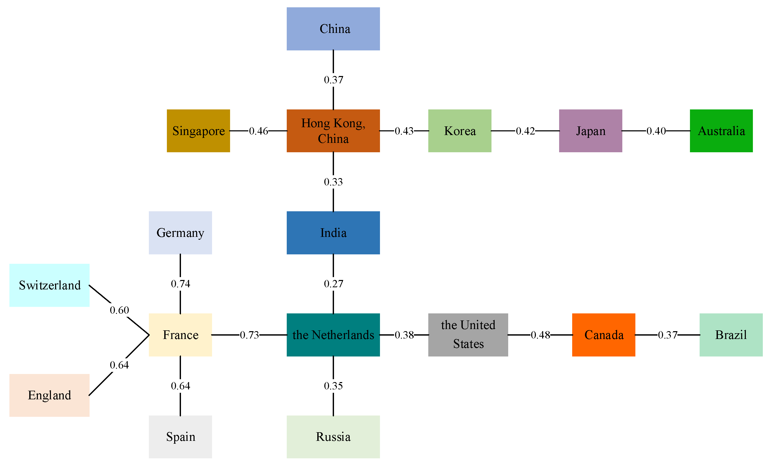
First, the R-Vine Copula modeling reveals that there is a distinct geographical feature of the global equity market risk diffusion phenomenon, i.e., countries and regions on the same continent are more closely connected to each other. Specifically, developed countries in Europe and the United States are at the center of the volatility spillover network, while other countries, especially emerging market countries, are at the edge of the volatility spillover network. This finding is consistent with Baumöhl et al. [61] and suggests that there is a clear regional dimension to the volatility spillover phenomenon of global equity market risk.

➢

Second, the development of equity market shows an uneven phenomenon globally, with more mature development of securities market in countries with a higher level of economic development. The net spillover effect of developed European countries is greater than 0, which reflects the output side of risk. The net spillover effect of other countries is less than 0, which indicates the input side of risk. Zhou et al. [62] measured the volatility spillover effects in the stock markets of Asian countries and other countries, and also found the same results. Unlike them, this paper considers the direction of risk spillovers and identifies the input side and output side of risk.

➢

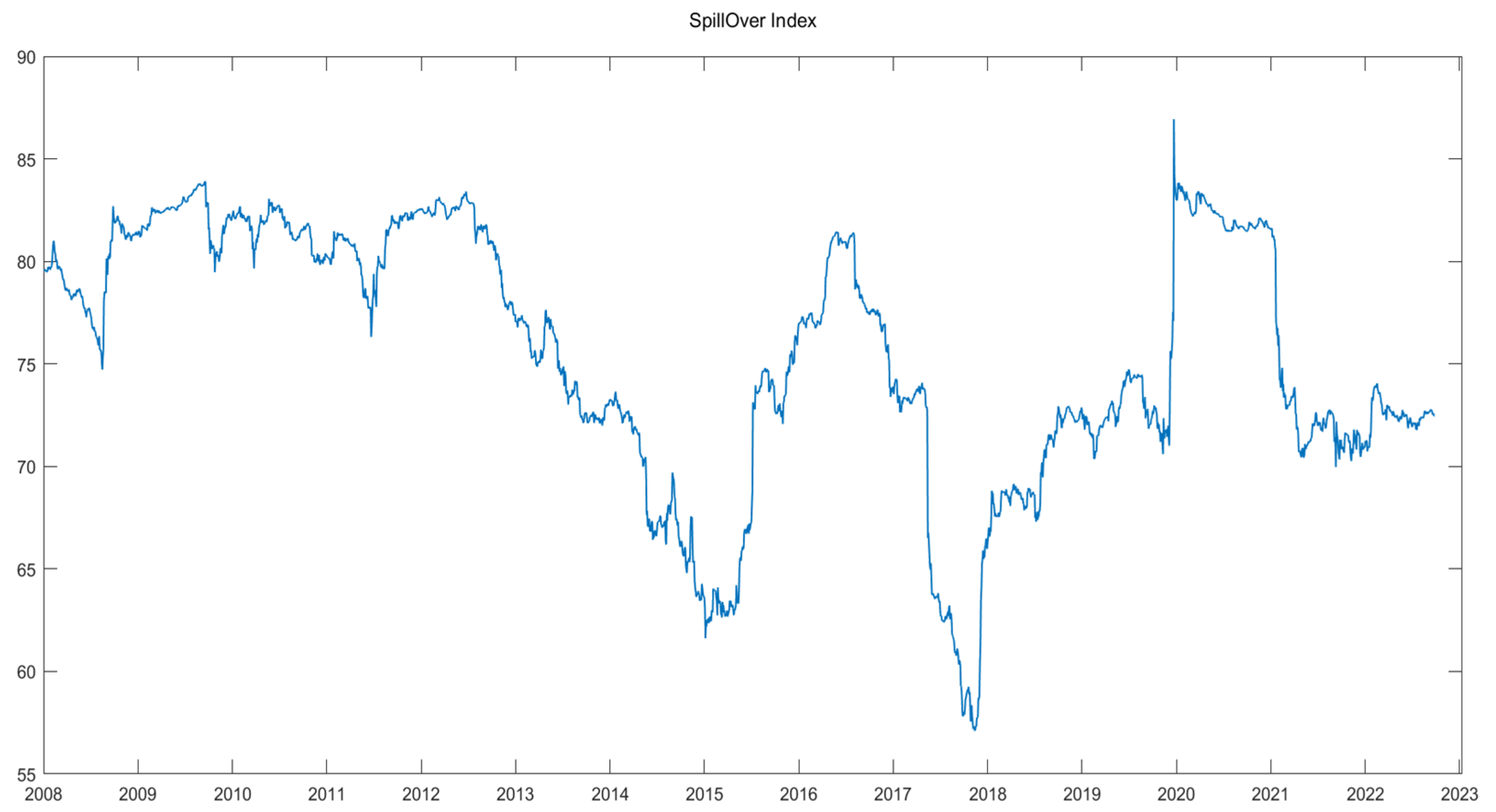
Finally, the rolling window method is used to measure the dynamic volatility spillover effect, and it is found that shocks from crisis events have an impact on the volatility spillover effect in equity markets. For example, during the subprime mortgage crisis, the European debt crisis, and the COVID-19 epidemic, the linkage among global equity markets increases significantly and the volatility spillover effect rises. Choi et al. [63] provided a dynamic measure of the volatility spillover effect across industries in the U.S. and reached similar conclusions. The difference is that the measurement results are more reflective of reality because they are based on the rolling window-based DY spillover index approach.

5. Conclusions

In this paper, we measured the global financial market volatility spillover effect using R-Vine Copula and the DY index, and constructed a global financial market volatility spillover network to analyze the global financial market volatility spillover effect and network diffusion. In general, the following conclusions can be summarized by analyzing the global financial market volatility spillover and network diffusion.

(1)

There is a certain aggregation feature in the network diffusion of global financial market volatility spillover. The entire network diffusion is centered on developed countries in Europe and the United States, with the remaining countries on the periphery.

(2)

Developed European countries such as the Netherlands, France, the UK, and Germany are at the center of the network and have a strong influence. Once a country’s financial market generates a volatile spillover of risk, it will cause a linkage reaction of risk in other important countries, and the network will become very rapidly connected.

(3)

Asian countries such as China, Japan, and India are at the periphery of the network. On the one hand, it is necessary for these countries to guard against the negative effects of risk volatility spillovers from important and key countries. On the other hand, it is also necessary for these countries to draw on the positive experience of financial market development to promote the development of their own national financial markets.

(4)

Shocks from crisis events can enhance volatility spillovers in global financial markets. During the subprime mortgage crisis, the European debt crisis, and the COVID-19 epidemic, the linkages in global financial market were enhanced, which led to an increase in volatility spillovers.

Since the network formed by the financial markets of each country is complex and diverse, the impact of the volatility spillover effects of the financial market risks of countries at the center of the network is huge. In addition, because they have strong linkages with other markets, it is easy to transmit the risk to other markets, making the risk expand further and finally triggering systemic risk. Therefore, effective prevention of risk volatility spillover and network diffusion in global financial markets and reduction in systemic risk need to be carried out in two ways:

(1)

Firstly, by focusing on the financial market of key countries in the network, such as the Netherlands, the UK, France, and Germany. Key markets are the center of risk diffusion in the network, and effective regulation of these markets can weaken the spread of risk to the greatest extent.

(2)

Second, the uneven development among global financial markets can be mitigated, reducing the high degree of correlation among financial markets. Market correlation is the basis for generating volatility spillover network diffusion. Reducing the correlation between markets and increasing the independence of each country’s financial market can effectively weaken network diffusion and prevent the accumulation of systemic risks.

Finally, there are some shortcomings in the study presented in this paper. For example, R-Vine Copula can only be used to study the symmetric volatility spillover effect among markets, and cannot reflect its directionality. Therefore, this paper introduces the DY spillover index to portray the directionality of the volatility spillover effect. However, determining how to better combine R-Vine Copula with the DY spillover index is something that needs further consideration. In addition, the choice of window width of the rolling window method based on the DY spillover index will have some influence on the results. How to eliminate this influence will also be the focus of the authors’ future research.

References

1. Li, Y.; Giles, D.E. Modelling volatility spillover effects between developed financial markets and Asian emerging financial markets. Int. J. Financ. Econ. 2015, 20, 155–177. [Google Scholar] [CrossRef] [Green Version]
2. Jebran, K.; Iqbal, A. Dynamics of volatility spillover between financial market and foreign exchange market: Evidence from Asian Countries. Financ. Innov. 2016, 2, 3. [Google Scholar] [CrossRef] [Green Version]
3. Christiansen, C. Volatility-Spillover Effects in European Bond Markets. Eur. Financ. Manag. 2007, 13, 923–948. [Google Scholar] [CrossRef]
4. Wu, F.; Guan, Z.; Myers, R.J. Volatility spillover effects and cross hedging in corn and crude oil futures. J. Futur. Mark. 2011, 31, 1052–1075. [Google Scholar] [CrossRef]
5. Zhou, W.; Gu, Q.; Chen, J. From volatility spillover to risk spread: An empirical study focuses on renewable energy markets. Renew. Energy 2021, 180, 329–342. [Google Scholar] [CrossRef]
6. Lee, S.J. Volatility spillover effects among six Asian countries. Appl. Econ. Lett. 2009, 16, 501–508. [Google Scholar] [CrossRef]
7. Katsiampa, P.; Corbet, S.; Lucey, B. Volatility spillover effects in leading cryptocurrencies: A BEKK-MGARCH analysis. Financ. Res. Lett. 2019, 29, 68–74. [Google Scholar] [CrossRef] [Green Version]
8. Calvo, G.A.; Mendoza, E.G. Rational contagion and the globalization of securities markets. J. Int. Econ. 2000, 51, 79–113. [Google Scholar] [CrossRef] [Green Version]
9. Adrian, T.; Brunnermeier, M.K. CoVaR (No. w17454). Am. Econ. Rev. 2011, 106, 1705–1741. [Google Scholar] [CrossRef]
10. Mink, M.; de Haan, J. Contagion during the Greek sovereign debt crisis. J. Int. Money Financ. 2013, 34, 102–113. [Google Scholar] [CrossRef]
11. Yang, J.; Zhou, Y. Credit Risk Spillovers Among Financial Institutions Around the Global Credit Crisis: Firm-Level Evidence. Manag. Sci. 2013, 59, 2343–2359. [Google Scholar] [CrossRef] [Green Version]
12. Troster, V.; Shahbaz, M.; Uddin, G.S. Renewable energy, oil prices, and economic activity: A Granger-causality in quantiles analysis. Energy Econ. 2018, 70, 440–452. [Google Scholar] [CrossRef] [Green Version]
13. Wen, D.; Wang, G.J.; Ma, C.; Wang, Y. Risk spillovers between oil and financial markets: A VAR for VaR analysis. Energy Econ. 2019, 80, 524–535. [Google Scholar] [CrossRef]
14. Ji, Q.; Bouri, E.; Roubaud, D.; Shahzad, S.J.H. Risk spillover between energy and agricultural commodity markets: A dependence-switching CoVaR-copula model. Energy Econ. 2018, 75, 14–27. [Google Scholar] [CrossRef]
15. Ardia, D.; Bluteau, K.; Rüede, M. Regime changes in Bitcoin GARCH volatility dynamics. Financ. Res. Lett. 2019, 29, 266–271. [Google Scholar] [CrossRef]
16. Fakhfekh, M.; Jeribi, A. Volatility dynamics of crypto-currencies’ returns: Evidence from asymmetric and long memory GARCH models. Res. Int. Bus. Financ. 2020, 51, 101075. [Google Scholar] [CrossRef]
17. Ali, G. EGARCH, GJR-GARCH, TGARCH, AVGARCH, NGARCH, IGARCH and APARCH models for pathogens at marine recreational sites. J. Stat. Econom. Methods 2013, 2, 57–73. [Google Scholar]
18. Lama, A.; Jha, G.K.; Paul, R.K.; Gurung, B. Modelling and Forecasting of Price Volatility: An Application of GARCH and EGARCH Models. Agric. Econ. Res. Rev. 2015, 28, 73–82. [Google Scholar] [CrossRef] [Green Version]
19. Bhatnagar, M.; Özen, E.; Taneja, S.; Grima, S.; Rupeika-Apoga, R. The Dynamic Connectedness between Risk and Return in the Fintech Market of India: Evidence Using the GARCH-M Approach. Risks 2022, 10, 209. [Google Scholar] [CrossRef]
20. Jones, P.M.; Olson, E. The time-varying correlation between uncertainty, output, and inflation: Evidence from a DCC-GARCH model. Econ. Lett. 2012, 118, 33–37. [Google Scholar] [CrossRef]
21. Yu, L.; Zha, R.; Stafylas, D.; He, K.; Liu, J. Dependences and volatility spillovers between the oil and financial markets: New evidence from the copula and VAR-BEKK-GARCH models. Int. Rev. Financ. Anal. 2020, 68, 101280. [Google Scholar] [CrossRef]
22. Zhang, Y.; Wang, M.; Xiong, X.; Zou, G. Volatility spillovers between stock, bond, oil, and gold with portfolio implications: Evidence from China. Financ. Res. Lett. 2021, 40, 101786. [Google Scholar] [CrossRef]
23. Chen, J.; Chen, Y.; Gu, Q.; Zhou, W. Network evolution underneath the volatility spillover in traditional and clean energy markets. Appl. Econ. 2023, 1–17. [Google Scholar] [CrossRef]
24. Fischer, M.; Köck, C.; Schlüter, S.; Weigert, F. An empirical analysis of multivariate copula models. Quant. Financ. 2009, 9, 839–854. [Google Scholar] [CrossRef] [Green Version]
25. Oh, D.H.; Patton, A.J. Time-Varying Systemic Risk: Evidence from a Dynamic Copula Model of CDS Spreads. J. Bus. Econ. Stat. 2018, 36, 181–195. [Google Scholar] [CrossRef] [Green Version]
26. Fang, L.; Balakrishnan, N.; Jin, Q. Optimal grouping of heterogeneous components in series–parallel and parallel–series systems under Archimedean copula dependence. J. Comput. Appl. Math. 2020, 377, 112916. [Google Scholar] [CrossRef]
27. Albulescu, C.T.; Tiwari, A.K.; Ji, Q. Copula-based local dependence among energy, agriculture and metal commodities markets. Energy 2020, 202, 117762. [Google Scholar] [CrossRef]
28. Pho, K.H.; Ly, S.; Lu, R.; Van Hoang, T.H.; Wong, W.-K. Is Bitcoin a better portfolio diversifier than gold? A copula and sectoral analysis for China. Int. Rev. Financ. Anal. 2021, 74, 101674. [Google Scholar] [CrossRef]
29. Ma, Y.; Wang, J. Co-movement between oil, gas, coal, and iron ore prices, the Australian dollar, and the Chinese RMB exchange rates: A copula approach. Resour. Policy 2019, 63, 101471. [Google Scholar] [CrossRef]
30. Dißmann, J.; Brechmann, E.; Czado, C.; Kurowicka, D. Selecting and estimating regular vine copulae and application to financial returns. Comput. Stat. Data Anal. 2013, 59, 52–69. [Google Scholar] [CrossRef] [Green Version]
31. Wang, Z.; Wang, W.; Liu, C.; Wang, Z.; Hou, Y. Probabilistic Forecast for Multiple Wind Farms Based on Regular Vine Copulas. IEEE Trans. Power Syst. 2017, 33, 578–589. [Google Scholar] [CrossRef]
32. Zhang, D.; Yan, M.; Tsopanakis, A. Financial stress relationships among Euro area countries: An R-vine copula approach. Eur. J. Financ. 2018, 24, 1587–1608. [Google Scholar] [CrossRef]
33. Schepsmeier, U. A goodness-of-fit test for regular vine copula models. Econ. Rev. 2019, 38, 25–46. [Google Scholar] [CrossRef] [Green Version]
34. Zhang, X.; Zhang, T.; Lee, C.-C. The path of financial risk spillover in the stock market based on the R-vine-Copula model. Phys. A Stat. Mech. Its Appl. 2022, 600, 127470. [Google Scholar] [CrossRef]
35. Zhou, W.; Chen, Y.; Chen, J. Risk spread in multiple energy markets: Extreme volatility spillover network analysis before and during the COVID-19 pandemic. Energy 2022, 256, 124580. [Google Scholar] [CrossRef]
36. Diebold, F.X.; Yilmaz, K. Measuring Financial Asset Return and Volatility Spillovers, with Application to Global Equity Markets. Econ. J. 2009, 119, 158–171. [Google Scholar] [CrossRef] [Green Version]
37. Diebold, F.X.; Yilmaz, K. Better to give than to receive: Predictive directional measurement of volatility spillovers. Int. J. Forecast. 2012, 28, 57–66. [Google Scholar] [CrossRef] [Green Version]
38. Tiwari, A.K.; Nasreen, S.; Ullah, S.; Shahbaz, M. Analysing spillover between returns and volatility series of oil across major financial markets. Int. J. Financ. Econ. 2021, 26, 2458–2490. [Google Scholar] [CrossRef]
39. Wang, H.; Li, S. Asymmetric volatility spillovers between crude oil and China’s financial markets. Energy 2021, 233, 121168. [Google Scholar] [CrossRef]
40. Fasanya, I.O.; Oyewole, O.; Odudu, T. Returns and volatility spillovers among cryptocurrency portfolios. Int. J. Manag. Financ. 2021, 17, 327–341. [Google Scholar] [CrossRef]
41. Gong, X.; Liu, Y.; Wang, X. Dynamic volatility spillovers across oil and natural gas futures markets based on a time-varying spillover method. Int. Rev. Financ. Anal. 2021, 76, 101790. [Google Scholar] [CrossRef]
42. Antonakakis, N.; Gabauer, D. Refined Measures of Dynamic Connectedness Based on TVP-VAR; Munich Personal RePEc Archive: Munich, Germany, 2017. [Google Scholar]
43. Antonakakis, N.; Cunado, J.; Filis, G.; Gabauer, D.; de Gracia, F.P. Oil volatility, oil and gas firms and portfolio diversification. Energy Econ. 2018, 70, 499–515. [Google Scholar] [CrossRef] [Green Version]
44. Boss, M.; Elsinger, H.; Summer, M.; Thurner, S. Network topology of the interbank market. Quant. Financ. 2004, 4, 677–684. [Google Scholar] [CrossRef] [Green Version]
45. Zou, Y.; Donner, R.V.; Marwan, N.; Donges, J.F.; Kurths, J. Complex network approaches to nonlinear time series analysis. Phys. Rep. 2019, 787, 1–97. [Google Scholar] [CrossRef]
46. Xu, H.; Wang, M.; Jiang, S.; Yang, W. Carbon price forecasting with complex network and extreme learning machine. Phys. A Stat. Mech. Its Appl. 2020, 545, 122830. [Google Scholar] [CrossRef]
47. Alavifard, F. Modelling default dependence in automotive supply networks using vine-copula. Int. J. Prod. Res. 2019, 57, 433–451. [Google Scholar] [CrossRef]
48. Xu, Q.; Fan, Z.; Jia, W.; Jiang, C. Fault detection of wind turbines via multivariate process monitoring based on vine copulas. Renew. Energy 2020, 161, 939–955. [Google Scholar] [CrossRef]
49. Marcot, B.G.; Penman, T.D. Advances in Bayesian network modelling: Integration of modelling technologies. Environ. Model. Softw. 2019, 111, 386–393. [Google Scholar] [CrossRef]
50. Algieri, B.; Leccadito, A. Assessing contagion risk from energy and non-energy commodity markets. Energy Econ. 2017, 62, 312–322. [Google Scholar] [CrossRef]
51. Khalfaoui, R.; Shahzad, U.; Asl, M.G.; Ben Jabeur, S. Investigating the spillovers between energy, food, and agricultural commodity markets: New insights from the quantile coherency approach. Q. Rev. Econ. Financ. 2023, 88, 63–80. [Google Scholar] [CrossRef]
52. Nekhili, R.; Bouri, E. Higher-order moments and co-moments’ contribution to spillover analysis and portfolio risk management. Energy Econ. 2023, 119, 106596. [Google Scholar] [CrossRef]
53. Trivedi, J.; Spulbar, C.; Birau, R.; Mehdiabadi, A. Modelling volatility spillovers, cross-market correlation and co-movements between stock markets in european union: An empirical case study. J. Bus. Manag. Econ. Eng. 2021, 19, 70–90. [Google Scholar] [CrossRef]
54. Sakthivel, P.; Bodkhe, N.; Kamaiah, B. Correlation and Volatility Transmission across International Stock Markets: A Bivariate GARCH Analysis. Int. J. Econ. Financ. 2012, 4, 253. [Google Scholar] [CrossRef]
55. Pal, D.; Mitra, S.K. Correlation dynamics of crude oil with agricultural commodities: A comparison between energy and food crops. Econ. Model. 2019, 82, 453–466. [Google Scholar] [CrossRef]
56. Chang, K.; Zhang, C.; Wang, H.W. Asymmetric dependence structures between emission allowances and energy markets: New evidence from China’s emissions trading scheme pilots. Environ. Sci. Pollut. Res. 2020, 27, 21140–21158. [Google Scholar] [CrossRef]
57. Patton, A.J. A review of copula models for economic time series. J. Multivar. Anal. 2012, 110, 4–18. [Google Scholar] [CrossRef] [Green Version]
58. Erhardt, T.M.; Czado, C.; Schepsmeier, U. R-vine models for spatial time series with an application to daily mean temperature. Biometrics 2015, 71, 323–332. [Google Scholar] [CrossRef] [Green Version]
59. Hernandez, J.A.; Hammoudeh, S.; Nguyen, D.K.; Al Janabi, M.A.M.; Reboredo, J.C. Global financial crisis and dependence risk analysis of sector portfolios: A vine copula approach. Appl. Econ. 2017, 49, 2409–2427. [Google Scholar] [CrossRef] [Green Version]
60. Czado, C.; Nagler, T. Vine copula based modeling. Annu. Rev. Stat. Its Appl. 2022, 9, 453–477. [Google Scholar] [CrossRef]
61. Baumöhl, E.; Kočenda, E.; Lyócsa, Š.; Výrost, T. Networks of volatility spillovers among stock markets. Phys. A Stat. Mech. Its Appl. 2018, 490, 1555–1574. [Google Scholar] [CrossRef] [Green Version]
62. Zhou, X.; Zhang, W.; Zhang, J. Volatility spillovers between the Chinese and world equity markets. Pac. -Basin Financ. J. 2012, 20, 247–270. [Google Scholar] [CrossRef]
63. Choi, S.-Y. Dynamic volatility spillovers between industries in the US stock market: Evidence from the COVID-19 pandemic and Black Monday. N. Am. J. Econ. Financ. 2022, 59, 101614. [Google Scholar] [CrossRef]
Figure 1. Risk spillover and diffusion relationships in the global financial market.
Mathematics 11 01396 g001
Figure 2. Dynamic risk spillover and diffusion in global financial market.
Mathematics 11 01396 g002