Financial Risk Measurement and Spatial Spillover Effects Based on an Imported Financial Risk Network: Evidence from Countries along the Belt and Road

Abstract

Using the financial market data of 35 countries along the Belt and Road (B&R), this paper constructs an imported financial risk network based on the conditional expected shortfall (CoES) to measure the systemic financial risk of the countries along the B&R. Furthermore, complex network theory is combined with spatial econometrics to construct a spatial, financial network panel model to measure the spatial spillover effects of imported financial risks and further explore the macroeconomic influences on systemic financial risks. The results show that among the countries along the B&R, the level of systemic financial risk in the European region is higher than that in the Asian region from the imported risk perspective. The spatial spillover effect of financial risk and the spatial spillover effect from the imported risk perspective have time-varying characteristics, with the spatial spillover effect increasing significantly during crisis periods. In addition, indicators of the three dimensions of economic openness, the institutional environment, and the external policy environment all have significant effects on systemic financial risk, but the effects differ across regions and periods.

1. Introduction

In September 2013, during a state visit to Kazakhstan, Chinese President Xi Jinping proposed the construction of the “Silk Road Economic Belt”. On October 3 of the same year, Xi Jinping delivered a speech at the Indonesian parliament, proposing the joint construction of the “21st Century Maritime Silk Road”. The “Silk Road Economic Belt” and the “21st Century Maritime Silk Road” constitute the “Belt and Road (B&R)” initiative. Along with the continuous promotion of the B&R initiative, cooperation among countries along the route in the fields of finance, trade, and investment has deepened, which has greatly promoted the economic and social development of each country. Until August 2022, China’s trade in goods with countries along the B&R has exceeded USD 12 trillion, and China’s investment in countries along the B&R has exceeded USD 140 billion. The continuous development of economic and trade cooperation along the B&R has promoted the improvement of infrastructure in the countries along the route and attracted many international investors. However, the cross-border flow of capital has also contributed to the contagion of financial risks in the countries along the route, which has increased the imported financial risks in these countries. This may lead to increased spatial spillover effects of financial risks in countries along the B&R.

The imported financial risk can be defined by portraying the contagion of financial risk. Because financial risks are contagious, financial risks in one country may be transmitted to other countries through trade, capital, geopolitical and other channels [1]. Therefore, we can divide the contagion process of financial risk into risk transmitters, risk transmission channels, and risk receivers. In the process of risk transmission, a country transmits financial risk to other countries through multiple channels, which can be called financial risk spillover. In turn, the external financial risk received by a country is imported financial risk [2]. Meanwhile, the impact of crisis events such as the “subprime crisis”, “European debt crisis” and “COVID-19 pandemic” in recent years has shown that there are significant spatial spillover effects of financial risks. In the discussion of financial risk, ignoring the spatial spillover effects of risk is one of the deficiencies in the measurement process [3]. In the current context of increasing uncertainties in the external environment and the frequent occurrence of crisis events, it is important to explore the imported financial risks and their spatial spillover effects in the countries along the B&R. This is not only beneficial for countries around the world, including China, to improve their development level, but also beneficial for investors in various countries to reduce risks and improve investment returns.

Therefore, it is of great academic value and practical significance to measure imported financial risks and their spatial spillover effects in countries along the B&R from the perspective of risk contagion and further analyze the influencing factors of systemic financial risks from three perspectives: the degree of economic openness, the institutional environment, and the external policy environment. This will not only help the countries along the B&R improve the level of financial supervision, effectively cope with imported financial risks and promote the long-term stability of their economies but also help promote the high-quality development of the B&R initiative.

After the subprime crisis, a large number of studies on systemic financial risk have emerged, but most of them have been conducted within developed countries or regional economic groupings, such as the G20 [4,5,6], BRICS [7,8,9], OECD or G7 countries [10,11,12,13]. There are relatively few studies focusing on financial risk contagion in countries along the B&R, and few studies measure systemic financial risk in countries along the B&R from the perspective of imported risk. Currently, scholars mainly use the generalized variance decomposition method to measure imported financial risk [14,15]. Regarding the measurement of systemic financial risk, most of the existing studies are based on equity returns. The indicators used mainly include expected loss (ES), value at risk (VaR), and others. Among them, ES indicators mainly include the systemic expected shortfall (SES), marginal expected shortfall (MES), and systemic risk index (SRISK) [16,17,18]. VaR indicators mainly include the conditional value at risk (CoVaR) and conditional expected shortfall (CoES) [19,20,21,22]. It has been shown that ES-type indicators are applicable for measuring the systemic financial risk of financial institutions, while VaR-type indicators can be applied for measuring systemic financial risk in financial markets [23].

The occurrence of systemic financial risks and their contagion effects are often closely related to systemically important financial institutions (SIFIs). Since the bankruptcy of Lehman Brothers, scholars have started to shift the criterion for identifying systemically important financial institutions from banks’ being “too big to fail” to banks’ being “too connected to fail”, and this shift is also applicable to the study of financial markets. In this context, complex network theory is increasingly being used to measure systemic financial risks in national financial markets from the perspective of risk contagion [24]. Most of these research approaches adopt the generalized vector autoregressive model (VAR) to construct the variance decomposition spillover index network or the CoVaR risk spillover network based on quantile regression. Compared with CoES, the variance decomposition spillover index focuses on the volatility spillover of financial risk and cannot portray the real risk spillover [25], while CoVaR is limited to the risk spillover in a single quantile, tending to underestimate the real risk spillover [26]. Therefore, a CoES-based imported financial risk network can accurately measure systemic financial risks and identify systemically important countries, providing a necessary reference for the development of the B&R initiative.

With the increasing spatial effects among countries’ financial markets, financial risk contagion shows obvious spatial characteristics [27]. Therefore, scholars have begun to combine spatial econometric theory with complex network theory to construct spatial econometric complex network models to measure the spatial spillover effects of financial risks [28]. With the wide application of information technologies such as the internet in the financial field, the speed of information spillover in financial markets has heightened, and the traditional physical distance matrix and adjacency matrix can no longer effectively measure the actual distance between each financial market [29] and thus also cannot effectively measure the spatial spillover effect of financial risk. Because copula functions can effectively portray the nonlinear tail dependence of financial market data, they are widely used to measure the economic distance among financial markets to measure the spatial spillover of financial risk [30,31]. However, a copula measures the economic distance between two financial markets as, by default, the same; i.e., the risk spillover from the financial market of country A to the financial market of country B is the same as the risk spillover from country B to country A. However, this is inconsistent with the facts, and thus it is necessary to measure the spatial spillover effects of financial risk using a spatial econometric financial network panel model, drawing on the asymmetric spatial weight matrix proposed by Cohen-Cole et al. [28].

In summary, research on systemic financial risk in countries along the B&R is still in its initial stage, and almost no research has been found on the use of the CoES method to construct an imported financial risk network to measure systemic financial risk. In addition, regarding the spatial spillover of financial risk, most scholars still use the tail correlation coefficient as a proxy variable for economic distance, ignoring the directionality of financial risk transmission, which easily leads to inaccurate measurement of spatial spillover effects. Regarding the prevention of systemic financial risks, scholars have focused mainly on developed countries or international financial markets, and there is little literature on the preventive measures of systemic financial risks from the perspective of countries along the B&R. Therefore, this paper treats the financial markets of the countries along the B&R as the carriers of imported financial risks. Firstly, we use the CoES method to construct an imported financial risk network, which is used to measure the level of systemic financial risk from the imported risk perspective of each country. Secondly, we introduce a risk distance measure to describe the spatial risk relationship among financial markets and construct the gravitational effect spatial weight matrix. A multidimensional spatial econometric model is used to measure the spatial spillover effect of financial risk from the imported perspective. Finally, we empirically analyze the factors influencing systemic financial risk from the imported perspective in three dimensions: economic openness, the institutional environment, and the external policy environment.

The major contributions of this paper are summarized as follows: (1) Most studies on the measurement of financial systemic risk focus on risk spillover or risk contagion, while spillover and contagion of financial systemic risk usually exist simultaneously. Considering the advantages of the CoES method in measuring financial systemic risk, we combine the CoES method with complex network theory to construct an imported financial risk network and examine the spillover and contagion of financial systemic risk at the same time. (2) Most studies on the spatial effects of financial risks mainly use symmetric matrices of physical or economic distances as spatial weight matrices, while risk spillovers among financial markets usually have asymmetric characteristics. We introduce a risk distance measure to replace traditional physical and economic distances and then construct an asymmetric spatial weight matrix to measure the spatial spillover effects of financial risks using a spatial econometric financial network panel model.

The remainder of this paper is organized as follows: Section 2 presents the research methodology, including the CoES method, imported financial risk network, the construction of the multidimensional risk space, and the multidimensional risk spatial regression model. Section 3 presents the data and the results of the empirical analysis, demonstrating the measurement results on systemic financial risks and the spatial spillover effects of financial risks and discussing the impact of macroeconomic factors on systemic financial risk. Section 4 concludes the paper.

2. Methodology

2.1. CoES

Imported financial risk can be understood as the risk spillover from other countries’ financial markets to domestic financial markets through international financial markets due to the linkage between countries’ financial markets [2]. For the measurement of imported financial risk, scholars mainly use the generalized variance decomposition network constructed based on the VAR model to measure imported financial risk, but since the VAR model cannot avoid the “dimensional disaster” caused by an excessive number of endogenous variables and cannot measure imported real risk, CoES is chosen to measure imported financial risk. Adrian et al. [32] have proposed the idea of CoES, and Zhang et al. [33] and Cui et al. [34] have refined the method for measuring systemic financial risk. CoES avoids the drawback of limiting CoVaR to risk spillovers in a single quantile, a method that tends to underestimate financial risk spillovers, while CoES based on quantile regression avoids the need for assumptions about the characteristics of the return distribution and improves the estimation precision. However, in terms of risk measurement, the above studies focus only on risk spillovers and ignore risk contagion. Therefore, we combine the CoES method with complex network theory to examine both the spillover and contagion of financial risks and then consider the good additivity of CoES [35], which can effectively improve the accuracy of measurement for imported financial risk.

Following the above idea and drawing on the study of Guo et al. [36], we focus the risk measure on two countries, country i and country j, and then calculate the CoES of the risk measure. Using the returns of the major stock market indices to denote the stock market boom indices of countries i and j, the return process of the stock markets of countries i and j can be expressed as Equations (1) and (2):

$$r_t^i={\alpha }_q^i+{\gamma }_q^i{M}_{t-1}+{\epsilon }_{q,t}^i$$

(1)

$$r_t^j={\alpha }_q^j+{\gamma }_q^j{M}_{t-1}+{\beta }_q^j{r}_t^i+{\epsilon }_{q,t}^j$$

(2)

where $r_t^i$, $r_t^j$ denote the log returns of the main stock indices of countries i and j, where the logarithmic return r_t = lnP_t − lnP_t−1, where P_t is the closing price of the main stock index and where M is a series of state variables that represent the movement of international financial markets, which are treated with a one-period lag to eliminate endogeneity among the state variables, denoted as M_t−1.

Further, since financial risk has a tail risk spillover effect, we obtain the tail risk spillover effect of the external state variable on the financial market of country i by running a q-quantile regression (q = 0.05) on Equations (1) and (2). The coefficients obtained from Equations (1) and (2) are again brought into Equations (3) and (4) to obtain the time-varying VaR and CoVaR.

$$Va{R}_{q,t}^i={\widehat{\alpha }}_{q,t}^i+{\widehat{\gamma }}_q^i{M}_{t-1}$$

(3)

$$CoVa{R}_{q,t}^{j|i}={\widehat{\alpha }}_q^j+{\widehat{\gamma }}_q^j{M}_{t-1}+{\widehat{\beta }}_q^{j}Va{R}_{q,t}^i$$

(4)

VaRⁱ_q,t denotes the value at risk for country i at the q quantile, and CoVaR^j|i_q,t denotes the conditional value at risk for country j when country i is in the risky state VaRⁱ_q,t. Since CoVaR only measures the risk spillover effect at the q quantile and ignores the extreme risk spillover beyond the q quantile, we further construct the conditional expected shortfall (CoES). According to the CoES definition defined by Adrian et al. [32], CoES can be expressed as

$$CoE{S}_{q,t}^{j|X^i=Va{R}_q^i}=E(X^j\le CoVa{R}_{q,t}^{j|C(X^i)}|Va{R}_{q,t}^i)$$

(5)

The meaning of Equation (5) is the expectation value when country i is in the risky state VaRⁱ_q,t and the stock index return of country j is less than CoVaR^j|i_q,t.

Further, the conditional expected risk in country j when country i is in the risky state VaRⁱ_q,t minus the conditional expected risk in country j when country i is in the normal state enables us to obtain the financial risk of country j imported from country i, which can be expressed as

$$\begin{array}{l}\Delta CoE{S}_{q,t}^{j|i}=CoE{S}_{q,t}^{j|X^i=Va{R}_q^i}-CoE{S}_{q,t}^{j|X^i=Va{R}_{0.5,t}^i}\\ \hspace{1em}\hspace{1em}\hspace{1em}\hspace{1em}=E(X^j\le CoVa{R}_{q,t}^{j|C(X^i)}|Va{R}_{q,t}^i)-E(X^j\le CoVa{R}_{0.5,t}^{j|C(X^i)}|Va{R}_{0.5,t}^i)\end{array}$$

(6)

Bringing Equation (5) into Equation (6), the financial risk of country j imported from country i can be expressed as

$$\Delta CoE{S}_{q,t}^{j|i}=E(X^j\le {\widehat{\beta }}_q^{j|i}(Va{R}_{q,t}^i-Va{R}_{0.5,t}^i))$$

(7)

To facilitate the comparison of indices across countries, we further nondimensionalize ∆CoES as follows:

$$\%\Delta CoES=\frac{\Delta CoE{S}_{q,t}^{j|i}}{E{S}_{q,t}^i}$$

(8)

Referring to the studies by Bai et al. [37] and Fang et al. [38], we use quantile regression, a rolling window, and historical simulation to estimate the dynamic CoES. Here, the rolling window is set to 220 days, and the following variables are chosen to constitute a series of state variables M: the global equity market sentiment index (Mr), which reflects the level of sentiment in global equity markets, as expressed by the log returns of the Global Equity Market Index (MSCI), published by Morgan Stanley Capital International; international equity market volatility (Mvar), which is represented by the standard deviation of the MSCI’s 22-day rolling returns; China’s manufacturing sentiment index (M_CMI), which captures the development of China’s foreign trade and is represented by the log returns of the SSE Industrial Index; the U.S. term spread (M_TS), which captures world macroeconomic fundamentals, expressed by the difference between the 10-year and 3-month U.S. Treasury yields to maturity; and interest rate trends (M_IRT), expressed by the difference between 3-month and 4-week U.S. Treasury yields.

2.2. Imported Financial Risk Network

Since ∆CoES takes into account only the spillover of financial risk and not the contagion of financial risk, we combine the CoES approach with complex network theory to measure systemic financial risk by constructing an imported financial risk network.

The imported financial risk network containing N country nodes can be denoted as G_T, where g_T^i→i and g_T^j→i denote the financial risk imported from country i to j and from country j to i in time period T, respectively, where:

$$g_T{}^{i\to j}=\frac{1}{T}{\displaystyle {\sum }_{t=1}^T\Delta CoE{S}_{q,t}^{j|i}}$$

(9)

$$g_T{}^{j\to i}=\frac{1}{T}{\displaystyle {\sum }_{t=1}^T\Delta CoE{S}_{q,t}^{i|j}}$$

(10)

Normally, country nodes do not generate imported financial risk to themselves, so the risk spillover g^i→i from country i to itself is 0. According to the above definitions, the adjacency matrix is used to represent the imported financial risk network G_T = (V_N,g_T) in time period T, where V_N = (1, 2, …, N) denotes the set of country nodes and g_T denotes the set of edges, so the adjacency matrix representation of the imported financial risk network G_T takes the form of Equation (9).

$$G_T=\left(\begin{array}{cccc}0& g_T{}^{1\to 2}& \cdots & g_T{}^{1\to N}\\ g_T{}^{2\to 1}& 0& ⋮& g_T{}^{2\to N}\\ ⋮& \cdots & \ddots & ⋮\\ g_T{}^{N\to 1}& g_T{}^{N\to 2}& \cdots & 0\end{array}\right)$$

(11)

It can be seen that the imported financial risk network G_T is a directional weighted network, and the degrees of nodes in the directional weighted network are divided into in-degree and out-degree. Therefore, drawing on the studies of Yang et al. [39], we define the systemic financial risk of country i in time period T from the perspective of imported risk as the in-degree of country node i in the imported financial risk network, which is denoted as

$$Srisk\text{-}i{n}_T^i={\displaystyle {\sum }_{j=1}^N{g}_T^{j\to i}}$$

(12)

Additionally, express the overall systemic financial risk in country i in time period T as the sum of the in-degree and out-degree of country node i in the imported financial risk network, which is denoted as

$$Srisk{\text{-}all}_T^i={\displaystyle {\sum }_{j=1}^N{g}_T^{j\to i}}+{\displaystyle {\sum }_{j=1}^N{g}_T^{i\to j}}$$

(13)

where T denotes the time horizon, Srisk-inⁱ_T denotes the systemic financial risk in country i from the imported risk perspective, and Srisk-allⁱ_T denotes the overall systemic financial risk in country i.

2.3. Multidimensional Risk Space

In previous studies, most scholars used “surface distance” and “adjacency distance” to measure the spatial correlation among financial markets, ignoring the multidimensional spatial spillover effects of financial risks. The element of the imported financial risk network G_T is used as the alternative variable for economic distance for each pair of countries, and it combines economic distance and surface distance through a nonlinear approach, which can effectively describe the multidimensional spillover of financial risks [40,41]. Based on this, we introduce the risk distance measure (RDM), which describes the spatial risk correlation among financial markets. Referring to the research of Li et al. [42], we construct the RDM in time period T, i.e., D_i,j,T between financial markets i and j, which can be expressed as:

$$D_{i,j,T}=F\left(G_{i,j,T},d_{i,j}\right)=\sqrt{1-{\left|G_{i,j,T}\right|}^{d_{i,j}}}\begin{array}{cc},& D_{i,j}\in \left[0,1\right]\end{array}$$

(14)

In Equation (12), G_i,j,T is the element of G_T that represents the risk spillover between financial markets i and j, $d_{i,j}\in \left[0,1\right]$; i.e., $d_{i,j}={d^{\prime }}_{i,j}/Max\left({d^{\prime }}_{i,j}\right)$ represents the relative physical distance between financial markets i and j.

Based on the defined RDM, we construct the gravitational effect spatial weights matrix in period T (denoted as W_T) by introducing the spatial gravity effect of the regional economy and combining the weight index of the geographical region and the weight index of the economic state. The diagonal elements of W_T are all 0, and the off-diagonal elements can be calculated by the following formula:

$$w_{i,j,T}=c_{i,j}\cdot \frac{m_i{m}_j}{\exp \left(D_{i,j,T}\right)}$$

(15)

where c_i,j is the control variable. In the process of establishing different types of spatial econometric models, c_i,j can be set as different economic indicators to reflect different economic meanings according to different problems in the financial field. D_i,j,T represents the RDM between financial markets i and j, m_i represents the proportion of the GDP of the i_th country in the total GDP value of all sample countries, and the control variable c_i,j is set equal to 1.

By the newly defined RDM and gravitational spatial weights matrix, we can construct the multidimensional risk space and then capture the multidimensional spatial effect. Furthermore, we test the existence of multidimensional spatial risk spillovers by estimating the spatial econometric regression model.

2.4. Multidimensional Risk Spatial Regression Model

Cohen-Cole et al. [28] and Elhorst [43] have provided continuous development and comprehensive presentations of spatial regression models. In the multidimensional risk space, we combine the spatial econometric model with the stock market returns of countries along the B&R to build the spatial financial network panel model. Assuming that there are N country nodes in the financial network, the spatial financial network panel model with a spatial lagged term can be expressed as follows:

$$y_{i,t}=\rho \frac{1}{w_{i,T}}{\displaystyle \sum _{j=1}^N{w}_{ij,T}{y}_{j,t}+}{\displaystyle \sum _{m=1}^M{\beta }^m}{x}_{i,t}^m+{\mu }_i+{\epsilon }_{i,t}$$

(16)

The spatial financial network panel model with a spatial error term can be expressed as follows:

$$\begin{array}{l}{y}_{i,t}={\displaystyle \sum _{m=1}^M{\beta }^m}{x}_{i,t}^m+{\mu }_i+u_{i,t}\\ u_{i,t}=\lambda \frac{1}{w_{i,T}}{\displaystyle \sum _{j=1}^N{w}_{ij,T}{u}_{i,t}+}{\epsilon }_{i,t}\end{array}$$

(17)

where w_i,j,T is an element of the gravitational effect spatial weight matrix W_Twith i = 1, 2, …, N; t = 1, 2, …, T; y_i,t denotes the return of the stock index of country i at time t; y_j,t denotes the corresponding return of the associated country j; ρ and λ are the spatial lags and spatial error coefficients, which denote the spatial spillover effects of financial risk; μ_i denotes the unit individual effects of national financial markets; and ε_i,t denotes the random error term, ε_i,t~N(0,σ²). Equations (16) and (17) can be further written in matrix form:

$$Y_t=\rho W{Y}_t+\beta X_t+{\mu }_i+{\epsilon }_t$$

(18)

$$Y_t=\beta X_t+\lambda W{\mu }_i+{\epsilon }_t$$

(19)

where Y_t is an N × 1 vector consisting of N country returns, W denotes the spatial weight matrix, and models (18) and (19) can be viewed as a spatial lagged financial network panel model and a spatial error financial network panel model, respectively. Before estimating models (18) and (19), the covariance function is chosen to perform a robust Hausman test on the ordinary panel OLS estimation results, and the results indicate that a fixed effects model should be chosen. Then, models (18) and (19) are estimated according to the maximum likelihood approach proposed by Elhorst [43].

3. Empirical Study and Results

3.1. Data Description

According to the literature, there are 65 countries or regions along the B&R, but due to the small size of individual countries’ stock markets and the unavailability of data, 35 countries are selected as the sample for this study. The GDP of the 35 sample countries accounts for 89.7% of the GDP of the 65 countries along the route, and the total foreign trade accounts for 87.7%. In addition, the 35 sample countries contain economies with different levels of development, which are representative. The daily closing prices of their major stock indices are used for the time window from 4 January 2006 to 15 June 2022. The missing values are interpolated using the moving average method to complete the data, resulting in 3996 sets of daily data. The relevant closing price data are obtained from the Bloomberg database, and the selected countries and the major stock indices of the country are given in

Table 1. List of 35 countries and stock indices.

Continent	Country	Symbol	Stock Index
Asia	China	CHN	CHN, CSI300 Index
Asia	Oman	OMN	OMN, MSM30 Index
Asia	Saudi Arabia	SAU	SAU, SASEIDX Index
Asia	Mongolia	MNG	MNG, MSETOP Index
Asia	Kazakhstan	KAZ	KAZ, KZKAK Index
Asia	Vietnam	VNM	VNM, VNINDEX Index
Asia	United Arab Emirates	UAE	UAE, ADSMI Index
Asia	India	IND	IND, SENSEX Index
Asia	Indonesia	IDN	IDN, JCI Index
Asia	Sri Lanka	LKA	LKA, CSEALL Index
Asia	Philippines	PHL	PHL, PCOMP Index
Asia	Thailand	THA	THA, SET Index
Asia	Pakistan	PAK	PAK, KSE100 Index
Asia	Singapore	SGP	SGP, STI Index
Asia	Jordan	JOR	JOD, JOSMGNFF Index
Asia	Korea, Rep.	KOR	KOR, KRX100 Index
Asia	Lebanon	LBN	LBN, BLOM Index
Europe	Cyprus	CYP	CYP, CYSMMAPA Index
Europe	Russian	RUS	RUS, CRTX Index
Europe	Greece	GRC	GRC, ASE Index
Europe	Hungary	HUN	HUN, BUX Index
Europe	Poland	POL	POL, WIG Index
Europe	Austria	AUT	AUT, ATXPRIME Index
Europe	Czech Republic	CZE	CZE, PX Index
Europe	Estonia	EST	EST, TALSE Index
Europe	Romania	ROU	ROU, BET Index
Europe	Latvia	LVA	LVA, RIGSE Index
Europe	Lithuania	LTU	LTU, VILSE Index
Europe	Bosnia and Herzegovina	BIH	BIH, BIRS Index
Europe	Croatia	HRV	HRK, CRO Index
Europe	Slovak Republic	SVK	SVK, SKSM Index
Australasia	New Zealand	NZL	NZL, NZSE50FG Index
America	Panama	PAN	PAN, BVPSBVPS Index
Africa	Egypt, Arab Rep.	EGY	EGY, HERMES Index
Africa	South Africa	ZAF	ZAF, JALSH Index

. In addition, the data of the selected state variables (see

Table 2. State variables for ∆CoES.

Variable Name	Symbol	Definition
Global equity market sentiment index	Mr	The log returns of the Global Equity Market Index (MSCI)
International equity market volatility	Mvar	The standard deviation of the MSCI’s 22-day rolling returns
China manufacturing sentiment index	MCMI	The log returns of the SSE Industrial Index
U.S. term spread	MTS	The difference between the 10-year and 3-month U.S. Treasury yields to maturity
Interest rate trends	MIRT	The difference between 3-month and 4-week U.S. Treasury yields

) are obtained from the iFind database, and the macro data of the countries along the B&R are obtained from the World Bank’s WDI database.

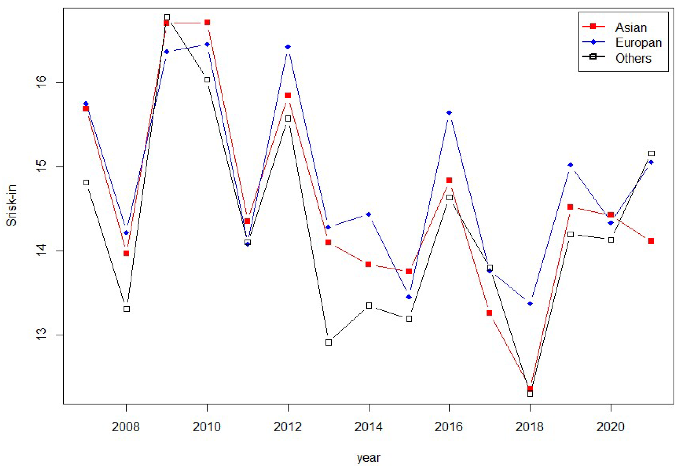
3.2. Measurement of Systemic Financial Risks

We set the time period T to one year and measure the annual Srisk-in of each country node by constructing an imported financial risk network and then analyzing the level of systemic financial risk from the imported risk perspective of each country.

Table 3. Results of systemic financial risk measurements.

2007	Rank	2010	Rank	2013	Rank	2016	Rank	2019	Rank	2021	Rank
IDN (20.13)	1	ROU (18.88)	1	GRC (20.36)	1	GRC (21.53)	1	GRC (19.69)	1	RUS (19.01)	1
PHL (18.69)	2	KAZ (18.79)	2	CYP (19.01)	2	ROU (18.58)	2	AUT (16.78)	2	EGY (17.25)	2
SGP (18.57)	3	EGY (18.64)	3	PHL (16.40)	3	HUN (18.56)	3	POL (16.27)	3	GRC (16.62)	3
IND (17.81)	4	IDN (18.42)	4	IDN (16.21)	3	EGY (17.63)	4	PHL (15.97)	4	VNM (16.42)	4
BIH (17.57)	5	IND (18.35)	5	THA (15.73)	4	IND (17.53)	5	IDN (15.95)	5	IND (16.29)	5
CHN (15.51)	20	CHN (16.57)	19	CHN (13.53)	19	CHN (13.91)	27	CHN (14.65)	19	CHN (14.33)	18

Note: Values in parentheses are Srisk-in measurements for each country node.

illustrates the top 5 countries in terms of Srisk-in for 2007, 2010, 2013, 2016, 2019, and 2021, as well as the Srisk-in of China and its ranking.

According to the results for different periods, when the “subprime crisis” broke out in 2007, Asian countries such as Indonesia, the Philippines, Singapore, and India had the highest Srisk-in. The main reason for this is that Asian countries have relatively late-developing financial markets, relatively inadequate financial systems, and small economies, so their risk resistance is weak. After the beginning of the European debt crisis in 2010, the highest Srisk-in was recorded in Romania, and with the outbreak of the European debt crisis in Greece and other countries, the Srisk-in measures of Greece, Cyprus, Romania, and other countries also rose one after another. After the end of the European debt crisis, the outbreak of Brexit also aggravated the rise of Srisk-in in European countries. Then, with the escalation of the Russia–Ukraine conflict, the Srisk-in measures of the relevant countries, including Russia, significantly exceeded those of other countries in 2021. At the same time, the Srisk-in of the emerging market country India is also ranked high, which is mainly related to its geopolitical and structural contradictions of economic development. Although China’s Srisk-in fluctuates in value, the ranking is basically stable and low, indicating that China is more resilient to risks. The international influence on the financial markets of China, which is the main driver of the B&R initiative, is still relatively weak, despite the country’s growing influence on the investment and trade sectors.

In addition, we divide the countries along the B&R into Asia, Europe, and other regions according to the continent where they are located. Figure 1 shows the Srisk-in for the three regions from 2007 to 2021, represented by the yearly average Srisk-in for all countries in each region. In general, the trend of systemic financial risk in the three regions remains consistent, indicating that Srisk-in is robust to systemic financial risk measures. At the same time, we find that the Srisk-in of each region is closely related to major regional events; the subprime crisis, European debt crisis, Brexit, the Russia–Ukraine conflict, and other crisis events have caused a significant rise in Srisk-in across regions.

Comparing the Asian region with the European region for the periods during the abovementioned crisis events, we can see that Srisk-in is significantly higher in the European region than in the Asian region because the European debt crisis, Brexit, and the Russia–Ukraine conflict mainly occurred in Europe, the European financial market developed earlier, and there was higher integration with the international market. At the same time, China, one of the largest economies and trade partners in the world, has played an important role in the stability of the Asian region’s economy, making the region’s Srisk-in smaller. In addition, the sample size of the other regions is relatively small, with only four countries, and their results will not be discussed here.

The results of the above analysis show that a country’s systemic financial risk exhibits significant time-varying characteristics under the combined effect of internal and external shocks. The systemic financial risk of a country reflects the stability of its economic structure. Countries with unstable economic structures are less able to cope with external shocks and have higher systemic financial risk. For investors, it may be more advantageous to implement prudent investment behavior in regions with higher systemic financial risk.

3.3. Spatial Spillover Effects of Financial Risks

The imported financial risk network reflects the risk spillover between countries along the B&R from the imported risk perspective, which can be represented by the adjacency matrix G_T. Since countries differ from each other in terms of risk spillovers, G_T is an asymmetric matrix. On this basis, we introduce the RDM to construct the gravitational effect spatial weight network W_T, which is used as a spatial weight matrix to measure the spatial spillover effect of financial risk from the imported risk perspective. Before constructing a spatial econometric financial network panel model, we first use the global Moran’s I for the spatial correlation test. In spatial econometrics, the classical global Moran’s I is only applicable to cross-sectional data and is no longer valid for panel data. Here, the spatial weight matrix in the classical global Moran’s I model is blocked: $K=I_T\otimes W$, where K is the NT × NT blocked diagonal matrix, I_T is the T-order identity matrix, W is the N-order spatial weight matrix, and $\otimes$ denotes the Kronecker product. The improved global Moran’s I can be extended to test for spatial effects in panel data, as calculated by the following equation:

$$\mathrm{Moran}’\mathrm{I}=\frac{N{\displaystyle \sum _{i=1}^N{\displaystyle \sum _{j=1}^N{k}_{i,j}\left(x_i-\overline{x}\right)\left(x_j-\overline{x}\right)}}}{{\displaystyle \sum _{i=1}^N{\displaystyle \sum _{j=1}^N{k}_{i,j}{\left(x_i-\overline{x}\right)}^2}}},\mathrm{Moran}’\mathrm{I}\in [-1,1]$$

(20)

Next, we introduce the low-volatility dummy variable (denoted as lvar) and the high-volatility dummy variable (denoted as hvar) to analyze the relationship between the spatial spillover effects of imported financial risk and the volatility of stock index returns. In order to obtain the lvar and hvar, we fitted the daily returns of all financial markets by using an ARMA(p,q)-GARCH model. The standard deviation of returns is used as a proxy variable for volatility, and the daily volatility is averaged into four groups. The first and fourth groups are used as lvar and hvar, respectively. The hvar is set to 1 for the high-volatility group and 0 for the low-volatility group; the lvar is set to the opposite values; and the values of the two middle reference groups remain unchanged. Then, the spatial spillover effect of financial risk is measured based on a spatial econometric financial network panel model.

Table 4. Estimated results of spatial correlation coefficients.

Year	Moran’s I	ρ	λ
2007	0.0925 *** (16.74)	0.1678 *** (9.03)	0.1678 *** (9.03)
2008	0.2087 *** (38.62)	0.3881 *** (26.7)	0.3877 *** (26.66)
2009	0.1388 *** (25.24)	0.3374 *** (21.8)	0.3374 *** (21.79)
2010	0.1552 *** (27.86)	0.3325 *** (21.4)	0.3325 *** (21.40)
2011	0.1463 *** (26.44)	0.4159 *** (30.03)	0.4162 *** (30.07)
2012	0.0684 *** (12.46)	0.2430 *** (14.01)	0.2434 *** (14.04)
2013	0.0934 *** (16.66)	0.2027 *** (11.19)	0.2027 *** (11.19)
2014	0.0583 *** (10.60)	0.1913 *** (10.57)	0.1881 *** (10.37)
2015	0.1779 *** (31.96)	0.1666 *** (9.04)	0.1666 *** (9.04)
2016	0.1356 *** (24.73)	0.2564 *** (15.04)	0.2565 *** (15.05)
2017	0.0404 *** (7.38)	0.1736 *** (9.36)	0.1736 *** (9.36)
2018	0.1040 *** (18.79)	0.1977 *** (10.95)	0.1973 *** (10.93)
2019	0.0824 *** (14.88)	0.1382 *** (7.28)	0.1384 *** (7.30)
2020	0.2252 *** (40.77)	0.5155 *** (43.78)	0.5161 *** (43.90)
2021	0.0591 *** (10.69)	0.1571 *** (8.38)	0.1569 *** (8.37)

Note: *** indicates significance at the 1% level; the corresponding z statistic or t statistic is in parentheses.

shows the annual Moran’s I and the results of the spatial spillover effect measures; the full estimated results of the spatial econometric financial network panel model are omitted here. The Moran’s I results for all years are significant at the 1% level, indicating that spatial spillover effects do exist for financial risk from the imported risk perspective while the spatial spillover effect ρ based on the spatial error model and the spatial spillover effect λ based on the spatial error model are almost the same in value and significant at the 1% level, indicating that the measures are more robust. In addition, Moran’s I, ρ, and λ are all positive, indicating that there is a significant positive spatial spillover effect for financial risk from the imported risk perspective.

The annual measurements in Table 4 show that the spatial spillover effect of financial risks reaches a phase peak in 2008, 2011, 2016, and 2020. These years correspond to the outbreaks of crisis events, such as the subprime crisis, the European debt crisis, Brexit, and the COVID-19 pandemic. This indicates that the occurrence of crisis events exacerbates the spatial spillover effects of financial risks, which will be further analyzed later. In addition, to confirm the time-varying characteristics of the spatial spillover effect of financial risk, we set the time period T to the whole sample period and then measure the time-varying risk spillover effect in a rolling 220-day window. The spatial spillover effects of the spatial lagged model (SLM) and the spatial error model (SEM) are given in Figure 2. The spatial spillover effect reflects the contagion of financial risk in terms of spatial correlation. Due to the contagious nature of financial risks, financial markets with similar RDMs may exhibit the same financial market volatility. In particular, when faced with shocks from crisis events, financial markets will show consistent volatility trends. Therefore, from Table 4 and Figure 2, we can find that financial risks exhibit significant spatial spillover effects and show a significant upward trend during the period of crisis events. It can be clearly found that the spatial spillover effect of financial risk is significantly higher during crisis periods and that the spatial spillover effects are higher during the COVID-19 pandemic than during the subprime crisis.

3.4. Impact Analysis of Crisis Events

To further analyze the systemic financial risk and spatial spillover of financial risk from the imported risk perspective during crisis periods, we set the sample intervals T₁ for the subprime crisis period (9 August 2007–8 December 2009), T₂ for the European debt crisis period (9 December 2009–3 June 2014), T₃ for the Brexit period (24 June 2016–17 October 2019), and T₄ for the COVID-19 pandemic period (15 January 2020–29 May 2020); the imported financial risk network is thereby constructed separately. Figure 3 illustrates the structure of imported financial risk networks during the above four crisis periods. The size of the nodes indicates the Srisk-in of each country, and the red nodes are the top 5 country nodes in the network. In addition,

Table 5. Systemic financial risk measures during crisis periods.

Subprime Crisis Period	European Debt Crisis Period	Brexit Period	COVID-19 Pandemic Period
Country nodes
Indonesia (19.63)	Cyprus (17.66)	Greece (17.40)	Greece (19.36)
Egypt (18.00)	Greece (17.12)	Hungary (15.79)	Egypt (16.37)
Saudi Arabia (17.90)	Indonesia (16.93)	Poland (15.54)	UAE (15.95)
Cyprus (17.06)	Egypt (16.65)	Russia (15.36)	Cyprus (15.43)
Philippines (16.97)	Kazakhstan (16.60)	Czech Republic (15.06)	Austria (15.27)
China (13.32)	China (14.56)	China (13.32)	China (14.16)
Regions
Asia region (15.36)	Asia region (15.11)	Asia region (14.76)	Asia region (13.65)
European region (15.44)	European region (15.38)	Europe region (13.24)	Europe region (14.38)
Other regions (14.95)	Other regions (14.58)	Other regions (12.43)	Other regions (13.70)
Overall level of sample countries
15.29	15.16	13.89	13.95

gives the Srisk-in results corresponding to the four crisis periods at three levels: country nodes, regions, and the sample countries as a whole.

The results in Figure 3 show that systemic financial risk increases in countries along the B&R during the period of crisis events. However, the shocks are different from one crisis event to another, and the systemic financial risk of each node in the imported financial risk network is not the same across the crisis events. Analyzing the characteristics of the top-ranked nodes, we can find that systemic financial risk is influenced by many factors, and it is not exclusively the shocks from crisis events that drive the rise in risk. When a country has structural problems in its economy or faces a more complex external environment, its systemic financial risk rises at a significantly higher level than that of other countries. This is because the emergence of internal crises leads to a reduction in the risk resistance of these countries. For example, during the European debt crisis, systemic financial risk rose in countries such as Greece. This was due to the high level of domestic debt that led to the bankruptcy of its government, which in turn led to a decline in its risk resistance.

In terms of country nodes, the five countries with the highest Srisk-in during the subprime crisis period were Indonesia, Egypt, Saudi Arabia, Cyprus, and the Philippines, with values of 19.63, 18.00, 17.90, 17.06, and 16.97, respectively. During the European debt crisis period, the top five countries with Srisk-in were Cyprus, Greece, Indonesia, Egypt, and Kazakhstan, with values of 17.66, 17.12, 16.93, 16.65, and 16.60, respectively. After that, during the Brexit period, the five countries with the highest Srisk-in values were Greece, Hungary, Poland, Russia, and the Czech Republic, with values of 17.40, 15.79, 15.54, 15.36, and 15.06, respectively. Finally, the top five countries with the highest Srisk-in values during the COVID-19 pandemic period were Greece, Egypt, United Arab Emirates, Cyprus, and Austria, with values of 19.36, 15.36, 15.36, and 15.06, respectively. Meanwhile, the Srisk-in of China in the above four periods was 13.32, 14.56, 13.32, and 14.16, ranking at 30, 24, 24, and 15, respectively.

In terms of the Srisk-in in different regions, during the subprime crisis period, the average risk levels in Asia, Europe, and other regions were 15.36, 15.44, and 14.95, respectively. The average risk levels in Asia, Europe, and other regions during the European debt crisis period were 15.11, 15.38, and 14.58, respectively. During the Brexit period, the numbers were 14.76, 13.24, and 12.43 in Asia, Europe, and other regions, respectively. During the COVID-19 pandemic period, the numbers were 13.65, 14.38, and 13.70 in Asia, Europe, and other regions, respectively. It can be found that Srisk-in was higher in Europe than in Asia and other regions in most crisis periods, consistent with the results of the annual analysis.

In addition, in terms of the overall level of sample countries, the overall Srisk-in of B&R countries was 15.29, 15.16, 13.89, and 13.95 in the four periods of the subprime crisis, the European debt crisis, Brexit, and the COVID-19 pandemic. The systemic financial risk of countries along the B&R was the highest during the subprime crisis, indicating that the impact of the global financial crisis on the international financial market was significantly higher than that of other crisis events.

Regarding the measurement of the spatial spillover effects of financial risks during crisis periods,

Table 6. Estimation results for crisis periods.

	SLM				SEM
	Subprime Crisis	European Debt Crisis	Brexit	COVID-19 Pandemic	Subprime Crisis	European Debt Crisis	Brexit	COVID-19 Pandemic
ρ	0.3766 *** (39.00)	0.3090 *** (41.12)	0.1886 *** (18.87)	0.5846 *** (34.67)
λ					0.3767 *** (39.01)	0.3090 *** (41.10)	0.1889 *** (18.90)	0.5862 *** (34.86)
lvar	−0.00033 (0.67)	−0.00034 * (−1.63)	−0.00011 (−0.61)	−0.00184 ** (−1.63)	−0.00040 (−0.62)	−0.00037 * (−1.70)	−0.00011 (−0.60)	−0.00158 * (−1.73)
hvar	0.00005 (0.11)	0.00020 ** (2.44)	0.00030 * (1.82)	0.00178 *** (1.69)	0.00014 (0.26)	0.00041 ** (2.04)	0.00030 * (1.84)	0.00217 * (1.81)
Fixed effects	Yes	Yes	Yes	Yes	Yes	Yes	Yes	Yes
Obs	19,950	38,605	28,245	3830	19,950	38,605	28,245	3830

Note: ***, **, and * indicate significance at the 1%, 5%, and 10% levels, respectively; corresponding t statistics are in parentheses.

shows the estimation results of a spatial financial network panel model for the four crisis periods. From the regression coefficients, the spatial spillover effect is positively correlated with high volatility and negatively correlated with low volatility, indicating that violent volatility in financial markets enhances the spatial correlation among countries, which may exacerbate the impact of crisis events. Meanwhile, the smooth development of financial markets can reduce the spatial spillover of imported financial risks and mitigate crises to some extent.

In terms of the spatial spillover effect of financial risk from the imported risk perspective, the highest spatial spillover effect is observed for the COVID-19 pandemic period at 0.742, followed by the effects for the subprime crisis period at 0.687 and for the Brexit period at 0.504, with the weakest effect appearing during the European debt crisis period at 0.596. In contrast to the dynamics of the spatial spillover effect, the average Srisk-in during the subprime crisis was larger than that during the COVID-19 pandemic. The reason for this is that the COVID-19 pandemic not only had an enormous impact on the financial markets of countries around the world but also inhibited the free flow of labor, production materials, and other factors on a global scale, which had a severe impact on the normal operation of global industrial and supply chains. The subprime crisis as a financial event mainly affected the global financial markets, while the development of internet communication technology made the spatial effect of the risk spillover between financial markets relatively weak.

3.5. Macroeconomic Influences on Systemic Financial Risk

3.5.1. Influence Mechanism and Empirical Model

Combined with existing studies, in terms of the macroeconomic influencing factors of systemic financial risk, we explore the impact of the three dimensions of economic openness, the institutional environment, and the external policy environment on systemic financial risk. The mechanism of their impact is shown in Figure 4.

Specifically, first, a higher degree of economic openness in a country or an economy is conducive to promoting the free flow of factors, such as means of production and capital, which in turn affect the transmission of financial risk across regions. A rise in external trade increases a country’s openness to the outside world, which in turn expands the country’s exposure to risk inputs and causes the accumulation of systemic financial risks [44]. The impact of cross-border capital flows on financial risk differs in the long and short term, with an increase in cross-border capital flows dampening systemic financial risk in the short term and having the opposite effect in the medium and long term [45]. Second, internal constraints in the institutional environment tend to affect the structure and smooth development of the economy. A reduction in economic freedom can lead to distortions in the economic structure, which in turn increases the possibility of a financial crisis [46]. The exchange rate regime is closely related to the stability of financial markets, and an appropriate exchange rate regime arrangement will contribute to smooth macroeconomic development, thus reducing a country’s financial vulnerability to a certain extent [47]. Third, the external policy environment faced by a country is characterized by high uncertainty, and its negative policy externalities are often prone to systemic financial risks. Global economic policy uncertainty is closely related to the outbreak of systemic financial risk in a country, which can cause a rapid accumulation of systemic financial risk by influencing a country’s macroeconomic policies and thus changing market expectations [48]). Global geopolitical risks can significantly affect stock market returns and ultimately lead to changes in systemic financial risk [49]. Therefore, the following variables are selected for empirical analysis (see

Table 7. Core explanatory variables.

Dimensions	Variable	Symbol	Definition
Economic openness	The growth rate of external openness	Growth-Opens	The ratio of total exports and imports to GDP of each country [50]
	The growth rate of short-term capital flows	Growth-SCF	Short-term capital flows expressed according to the residual method proposed by the World Bank, i.e., the ratio of net foreign direct investment inflows to GDP [51]
Institutional environment	Degree of economic freedom	Degree-Free	Published by the Wall Street Journal and the Heritage Foundation, contains 10 subindicators, including finance, investment, trade, etc. The values range from 0 to 100, and the higher the value, the freer the economy is
	Fixed exchange rate regime Intermediate exchange rate regime Floating exchange rate regime	Fixed Intermediate Floating	The exchange rate regime, including fixed, intermediate, or floating, is divided according to the 10 exchange rate regimes proposed by the IMF and the World Bank (Exchange rate regimes are divided according to the 10 exchange rate regimes proposed by the IMF of the World Bank, among which the fixed exchange rate regime includes “stabilized arrangement exchange rate system”, “traditional pegged exchange rate system”, “currency board system” and “no independent legal tender”. The intermediate exchange rate regime includes the “other exchange rate regime”, the “in-range crawling peg”, the “crawling arrangement exchange rate regime” and the “crawling peg”. “crawling peg”, and floating exchange rate regimes include “managed floating exchange rate regimes” and “full floating exchange rate regimes”.)
External policy environment	Economic policy uncertainty	GEPU	The economic and political uncertainty index constructed by Baker et al. [52] is used to measure global economic and political uncertainty (China Economic Policy Uncertainty Index from https://economicpolicyuncertaintyinchina.weebly.com/ (accessed on 6 October 2022).)
	Geopolitical risk index	GPR	The geopolitical risk index based on news reports proposed by Caldarahe et al. [53] (Global Geopolitical Risk Index from https://www.matteoiacoviello.com/gpr.htm (accessed on 6 October 2022).)

Note: (1) Since the degree of economic freedom is a monthly value, the annual average value is used to indicate the degree of economic freedom in that year. (2) Since the economic and political uncertainty index and geopolitical risk index are monthly data, annual averages are taken.

).

The impact of the above variables on systemic financial risk is analyzed empirically through a panel regression model, with the time window of the sample being 2007 to 2020 due to the availability of data. The panel regression model is set as shown in Equation (19).

$$y_{i,t}={\beta }_1+{\displaystyle \sum _{l=1}^L{\beta }_2{x}_{i.t,l}}+{\beta }_3{\displaystyle {\sum }_{h=1}^{H}contro{l}_{i,t,h}}+{\epsilon }_{it}$$

(21)

i denotes the countries along the B&R; t denotes the year; y is the dependent variable, denoted by the measure of systemic financial risk Srisk-in; and x is the core explanatory variable, as shown in Table 7. To prevent model estimation bias caused by omitted variables, control variables (control) are introduced here, including the GDP chain growth rate, government expenditure chain growth rate, broad money chain growth rate, local currency value chain growth rate (chain growth rate of the national currency against the US dollar), consumer price index chain growth rate, and consumption share of GDP.

3.5.2. Regression Results and Robustness Test

Table 8. Estimation results.

	(1)	(2)	(3)	(4)	(5)	(6)	(7)	(8)	(9)
C	15.744 *** (29.09)	15.681 *** (29.73)	18.392 *** (16.78)	15.16 *** (28.92)	15.80 *** (30.22)	16.238 *** (30.55)	21.654 *** (32.62)	26.305 *** (32.62)	26.953 *** (20.69)
Growth-Opens	−1.518 *** (2.63)							−1.661 ** (−3.81)	−1.661 ** (−3.81)
Growth-SCF		0.014 ** (2.13)						0.014 * (1.93)	0.014 * (1.93)
Degree-Free			−0.032 *** (−2.67)					−0.031 ** (−2.46)	−0.031 ** (−2.46)
Floating				0.639 ** (4.42)				0.647 *** (4.24)
Intermediate				0.312 ** (2.06)	−0.639 ** (−4.42)			0.118 (0.77)	−0.530 ** (−3.45)
Fixed					−0.327 ** (−2.07)				−0.648 ** (−4.24)
GEPU						−0.004 *** (−6.25)		−0.007 ** (−8.51)	−0.007 ** (−8.51)
GPR							−0.063 ** (−17.67)	−0.077 ** (−17.67)	−0.076 ** (−13.93)
Control	Yes	Yes	Yes	Yes	Yes	Yes	Yes	Yes	Yes
Mixed effect	Yes	Yes	Yes	Yes	Yes	Yes	Yes	Yes	Yes
Obs	490	490	490	490	490	490	490	490	490

Note: ***, **, and * indicate significance at the 1%, 5%, and 10% levels, respectively; corresponding t statistics are in parentheses; “C” indicates a constant term.

presents the regression results for the core explanatory variables. In terms of external openness, i.e., models (1) and (2), Growth-Opens has a negative effect on Srisk-in, probably because most of the countries along the B&R are export-oriented, and an increase in external openness benefits trade, which in turn boosts their economic growth and thus enhances their overall resistance to systemic financial risks. Growth-SCF has a positive effect on Srisk-in, indicating that a rise in cross-border capital flows expands a country’s risk exposure, leading to more exposure to imported financial risks and hence a rise in its systemic financial risk.

From the perspective of the institutional environment, i.e., models (3), (4), and (5), the negative effect of Degree-Free on Srisk-in may be explained by the fact that the higher the degree of economic freedom, the more dynamic a country’s market economy is, and the more flexible is its policy regulation when financial markets are volatile.

In terms of the exchange rate regime, a country’s resilience to systemic financial risk is enhanced when it has a fixed and intermediate exchange rate, while its resilience to systemic financial risk is reduced when it has a floating and intermediate exchange rate. This may be because a floating exchange rate regime is associated with greater volatility in the local currency, and sharp fluctuations in the exchange rate market can affect a country’s import and export trade, which can lead to disruptions in the development of the real economy and can easily trigger capital outflows and thus have a strong impact on the stock market.

From the perspective of the external policy environment, i.e., models (6) and (7), GEPU has a negative effect on Srisk-in because increased economic policy uncertainty induces a country to adopt flexible policy instruments to respond to financial market volatility and thus effectively cope with systemic financial risks. GPR has a negative effect on Srisk-in because rising global geopolitical risks increase a country’s imported risk to some extent. Such risks tend to be predictable, and the expectation of their realization prompts a country to adopt more aggressive fiscal and monetary policies to stabilize financial markets, thus enhancing the country’s risk resilience.

In addition, models (8) and (9) offer regression estimates, including all variables; the direction of the sign of the estimated coefficients of each core explanatory variable is consistent with the results obtained in regression models (1) to (7).

To avoid potential pseudoregressions, we replaced the explanatory variables with Srisk-all as a robustness test. The test results are given in

Table 9. Robustness test.

	(1)	(2)	(3)	(4)	(5)	(6)	(7)	(8)	(9)
C	31.001 *** (1.25)	31.026 *** (25.07)	26.824 *** (10.74)	29.95 *** (22.50)	31.924 *** (24.02)	32.701 *** (26.06)	43.004 *** (30.16)	43.73 *** (15.56)	45.555 *** (15.98)
Growth-Opens	−1.089 * (−1.70)							−1.824 ** (−2.34)	−1.824 ** (−2.35)
GrowthSCF		0.030 ** (2.09)						0.040 *** (2.83)	0.014 * (2.83)
Degree-Free			−1.76 *** (−2.67)					−0.029 * (−0.98)	−0.029* (−0.98)
Floating				1.972 *** (6.35)				1.822 *** (5.68)
Intermediate				0.712 ** (2.64)	−1.971 ** (−6.36)			0.328 (1.17)	−1.493 ** (−5.13)
Fixed					−1.259 *** (−4.34)				−1.821 *** (−5.68)
GEPU						−0.010 * (−5.44)		−0.015 ** (−6.87)	−0.015 ** (−6.87)
GPR							−0.132 ** (−18.45)	−0.152 ** (−15.12)	−0.152 ** (−15.12)
Control	Yes	Yes	Yes	Yes	Yes	Yes	Yes	Yes	Yes
Pooling effect	Yes	Yes	Yes	Yes	Yes	Yes	Yes	Yes	Yes
Obs	490	490	490	490	490	490	490	490	490

Note: ***, **, and * indicate significance at the 1%, 5%, and 10% levels, respectively; corresponding t statistics are in parentheses; “C” indicates a constant term.

. The results are still significant after we replace the explanatory variables, and there is no change in the positive and negative signs of the estimated coefficients, indicating that the previous results are robust and reliable.

3.5.3. Regional Heterogeneity Analysis

Since there is regional heterogeneity in the impact of macroeconomic factors on systemic financial risk, this section divides the countries along the B&R into Asia, Europe, and other regions to analyze the impact of systemic financial risk in different regions. Since the sample of countries in regions other than Asia and Europe is relatively small, these countries are not included in the regression analysis here.

The regression results for the different regions are given in

Table 10. Regional heterogeneity test results.

	(1)	(2)	(3)	(4)	(5)	(6)	(7)	(8)	(9)
Asia region
C	15.983 *** (99.58)	16.212 *** (129.31)	16.654 *** (29.24)	16.039 *** (149.80)	16.869 *** 154.48)	16.958 *** (105.27)	22.772 *** (49.12)	25.280 *** (22.82)	25.945 *** (23.19)
Growth-Opens	−3.82 *** (−16.33)							−3.141 ** (−7.86)	−3.141 ** (−7.86)
Growth-SCF		0.018 ** (3.16)						0.022 * (1.97)	0.022 * (1.97)
Degree-Free			−0.006 (−1.05)					−0.029 * (−0.98)	−0.029 * (−0.98)
Floating				0.839 *** (6.35)				0.665 *** (6.43)
Intermediate				−0.242 ** (−6.15)	−1.082 *** (−22.20)			−0.384 *** (−4.79)	−1.050 ** (−9.72)
Fixed					−0.839 ** (−18.86)				−0.666 *** (−6.43)
GEPU						−0.004 *** (−8.35)		−0.008 ** (−6.33)	−0.008 ** (−6.33)
GPR							−0.070 *** (−16.29)	−0.081 ** (−10.93)	−0.081 ** (−10.93)
Control	Yes	Yes	Yes	Yes	Yes	Yes	Yes	Yes	Yes
Pooling effect	Yes	Yes	Yes	Yes	Yes	Yes	Yes	Yes	Yes
Obs	238	238	238	238	238	238	238	238	238
European region
C	14.586 *** (36.56)	14.725 *** (146.14)	23.488 *** (30.12)	12.151 *** (37.16)	13.191 *** (43.01)	15.142 *** (41.31)	20.372 *** (29.62)	31.194 *** (30.84)	31.959 *** (31.63)
Growth-Opens	0.20 (0.75)							−0.172 (−0.68)	−0.172 (−0.68)
Growth-SCF		0.024 ** (49.07)						0.026 *** (11.98)	0.026 *** (11.98)
Degree-Free			−0.089 *** (−12.87)					−0.097 * (−12.86)	−0.097 * (−12.86)
Floating				1.040 *** (14.33)				0.765 *** (10.24)
Intermediate				0.021 ** (0.21)	−1.019 *** (−12.67)			−0.791 *** (−8.72)	−1.493 ** (−10.24)
Fixed					−1.040 ** (−14.33)				−1.557 *** (−18.16)
GEPU						−0.002 *** (−2.57)		−0.006 ** (−5.91)	−0.006 ** (−5.91)
GPR							−0.055 *** (−14.40)	−0.067 ** (−14.78)	−0.067 ** (−14.78)
Control	Yes	Yes	Yes	Yes	Yes	Yes	Yes	Yes	Yes
Pooling effect	Yes	Yes	Yes	Yes	Yes	Yes	Yes	Yes	Yes
Obs	196	196	196	196	196	196	196	196	196

Note: ***, **, and * indicate significance at the 1%, 5%, and 10% levels, respectively; corresponding t statistics are in parentheses; “C” indicates a constant term.

. In terms of effect heterogeneity, the effect of Growth-Opens on Srisk-in is negative in the Asian region and not significant in the European region. The main reason lies in their different modes of economic growth: Asian countries’ economic growth in recent years has been closely related to their degree of openness to the outside world. The impact of Degree-Free on Srisk-in is insignificant in the Asian region and negative in the European region. The reason for this is that countries in the Asian region have less economic freedom, and most Asian countries developed their market economies later. Thus, protection against systemic financial risk is mainly implemented through the government rather than through a reliance on the market economy to self-regulate.

In terms of the homogeneity of the impact effect, Growth-SCF and floating exchange rates have a positive impact on Srisk-in in both regions, while fixed exchange rates and the external policy environment factors GEPU and GPR have a negative impact on Srisk-in in both the European and the Asian region. This is consistent with the results of the regression analysis for the full sample of countries.

3.5.4. Further Analysis: The Shock Effects of Crisis Events

To further analyze the robustness of the shock effect, the impact of crisis events on systemic financial risk is discussed in this section. We set “subprime crisis”, “European debt crisis”, “Brexit”, and “COVID-19 pandemic” as dummy variables for crisis events, denoted by Crisis.

Table 11. Estimation results of the shock effects of crisis events.

	(1)	(2)	(3)	(4)	(5)
C	15.161 *** (28.26)	15.063 *** (28.26)	17.83 *** (15.96)	13.338 *** (23.87)	22.25 *** (25.40)
Crisis	1.293 *** (11.54)	1.278 *** (11.72)	1.850 *** (2.22)	3.693 *** (30.45)	3.94 *** (4.51)
Growth-Opens	−1.798 *** (−2.80)
Crisis × Growth-Opens	0.092 (0.12)
Growth-SCF		−0.004 (−0.32)
Crisis × Growth-SCF		0.029 * (1.95)
Degree-Free			−0.032 * (−2.57)
Crisis × Degree-Free			−0.009 (−0.70)
GEPU				0.009 *** (7.45)
Crisis × GEPU				−0.014 *** (−8.42)
GPR					−0.071 ** (−10.78)
Crisis × GPR					0.049 *** (5.27)
Control	Yes	Yes	Yes	Yes	Yes
Pooling effect	Yes	Yes	Yes	Yes	Yes
Obs	490	490	490	490	490

Note: ***, **, and * indicate significance at the 1%, 5%, and 10% levels, respectively; corresponding t statistics are in parentheses; “C” indicates a constant term.

shows the regression results for the interaction term of Crisis with the core explanatory variables. Since the exchange rate regime is a dummy variable, it is not introduced here in the regression analysis.

The estimation results show that the coefficient of Crisis is significantly positive, indicating that the level of systemic financial risk rises when a crisis event occurs. From the perspective of economic openness, the coefficient of Crisis × Growth-Opens is not significant. During a crisis, international trade can boost a country’s economic growth and thus reduce its systemic financial risk (Growth-Opens has a negative effect), but the financial risk can also enter the country through trade channels and thus increase its systemic financial risk. The combination of these two effects leads to an insignificant effect of Crisis × Growth-Opens. Meanwhile, the coefficient of Crisis × Growth-SCF is significantly positive. This is explained by the fact that cross-border capital flows expand a country’s risk exposure during crisis events, which contributes to the increase in the level of systemic financial risk.

From the perspective of the institutional environment, the regression coefficient of Crisis × Degree-Free is not significant. The potential reason for this is that countries with higher economic freedom have relatively weaker institutional protection for their domestic economies. During the period of crisis events, countries with higher economic freedom will be affected more dramatically, but they also have relatively stronger economic resilience and risk buffers, giving them the ability to restrain systemic financial risk.

In terms of the external policy environment, the coefficient of Crisis × GEPU is significantly negative. This suggests that economies can adopt more flexible fiscal and monetary policies to dampen shocks from crisis events, which can reduce their systemic financial risk. The coefficient of Crisis × GPR is significantly positive. It indicates that the outbreak of a crisis event makes the risk imported from geopolitical risk exceed the limits of the country’s policy buffers. Consequently, Crisis × GPR has a positive effect on Srisk-in.

4. Conclusions

In recent years, uncertainties in global economic development have increased, and waves of counter-globalization have been rising and falling. International economic, trade and investment cooperation, such as the B&R Initiative, has encountered various obstacles. The sustainable and stable development of financial markets in countries along the B&R is constantly challenged, and how to deal with imported financial risks effectively is a major challenge for the regulatory authorities of each country. Therefore, this paper constructs an imported financial risk network to measure the systemic financial risks of the countries along the B&R effectively and analyzes the spatial spillover effects of the financial risks from the imported risk perspective, based on which the macroeconomic impact factors of systemic financial risks are discussed. The results of the study are as follows:

(1) There are obvious regional differences in the level of systemic financial risk from the imported risk perspective of countries along the B&R. From a country perspective, countries in the Asian region, such as the Philippines, India, and Indonesia, and countries in the European region, such as Greece, Romania, Cyprus, Austria, and Poland, have higher levels of systemic financial risk. From a regional perspective, the systemic financial risk in Europe has been significantly higher than that in Asia, especially during the European debt crisis and Brexit periods. (2) The spatial spillover effect of financial risks from the imported risk perspective has obvious time-varying characteristics. When a crisis event occurs, the spatial spillover effect rises significantly and then declines significantly. Specifically, the spatial spillover effect of financial risk was highest during the COVID-19 pandemic period, followed by the subprime crisis period. The spatial spillover effects were weaker during the European debt crisis and Brexit periods, and the spillover effects were basically the same in both periods. In addition, the high volatility of the stock market during crises has an enhancing effect on the spatial spillover of financial risks, and the low volatility has a suppressing effect. (3) Macroeconomic factors in the three dimensions of economic openness, the institutional environment, and the external policy environment affect the level of systemic financial risk in countries along the B&R. Short-term capital flows and floating exchange rate regimes have significant positive effects, and fixed exchange rate regimes and factors in the external policy environment dimension have negative effects, while there is significant regional heterogeneity in the effects of factors such as the degree of external openness and economic freedom. Moreover, after introducing the dummy variable of crisis events, we can find that the systemic financial risk of each country rises significantly in response to crisis events. The research results suggest that cross-border capital flows and geopolitical risks promote systemic financial risk during crisis events, while economic policy uncertainty resists systemic financial risk.

Based on the above findings, the following countermeasures are proposed: (1) Caution is needed in investing in countries with high systemic financial risks. National regulators should establish targeted risk early warning mechanisms and focus on preventing possible risk contagion from countries with high systemic financial risks. (2) Effective prevention of the spatial spillover of financial risks is needed. From the perspective of the spatial spillover path of financial risks, financial risks can have a contagion effect along the imported financial risk network. Turmoil in the international financial market is the main driving force behind the enhancement of the spatial spillover effect of financial risks. Turmoil in both European and international financial markets strengthens the spatial spillover of financial risks in countries along the B&R. Therefore, maintaining the stable development of the world economy and highlighting China’s role as a stabilizer in global economic development is an important way to promote the rapid development of the B&R initiative. (3) Countries need to implement stable economic policies and exchange rate regimes and continuously develop higher-quality openness to the outside world. Countries should maintain a cautious attitude toward cross-border capital flows and actively address the risk exposures arising from these flows. In addition, in view of the three dimensions of economic openness, the institutional environment, and the external policy environment, countries along the B&R need to be cautious of imported financial risks arising from capital market opening and trade liberalization in the process of promoting the B&R initiative, expanding external openness and enhancing international cooperation.

References

1. Fang, Y.; Shao, Z.Q. Measurement of Imported Financial Risk under Major Shocks. Econ. Sci. 2022, 248, 13–30. [Google Scholar]
2. Yang, H.F.; Wang, W.F.; Wang, Y.X. Imported financial risk in China: Measurement, affecting factors and sources. J. Quant. Tech. Econ. 2020, 37, 113–133. [Google Scholar]
3. Chen, S.W.; Guo, L.; Qiang, Q. Spatial Spillovers of Financial Risk and Their Dynamic Evolution: Evidence from Listed Financial Institutions in China. Entropy 2022, 24, 1549. [Google Scholar] [CrossRef]
4. Liu, X.Y.; An, H.Z.; Li, H.J.; Chen, Z.H.; Feng, S.D.; Wen, S.B. Features of spillover networks in international financial markets: Evidence from the G20 countries. Phys. A Stat. Mech. Its Appl. 2017, 479, 265–278. [Google Scholar] [CrossRef]
5. Liu, B.Y.; Fan, Y.; Ji, Q.; Hussain, N. high-dimensional CoVaR network connectedness for measuring conditional financial contagion and risk spillovers from oil markets to the G20 stock system. Energy Econ. 2022, 105, 105749. [Google Scholar] [CrossRef]
6. Yousaf, I.; Patel, R.; Yarovaya, L. The reaction of G20+ stock markets to the Russia-Ukraine conflict “black-swan” event: Evidence from event study approach. J. Behav. Exp. Financ. 2022, 35, 100723. [Google Scholar] [CrossRef]
7. Naeem, M.A.; Pham, L.; Senthilkumar, A.; Karim, S. Oil shocks and BRIC markets: Evidence from extreme quantile approach. Energy Econ. 2022, 108, 105932. [Google Scholar] [CrossRef]
8. Ma, X.X.; Zong, X.Y.; Chen, X.M. Economic fitness and economy growth potentiality: Evidence from BRICS and OECD countries. Financ. Res. Lett. 2022, 50, 103235. [Google Scholar] [CrossRef]
9. Mensi, W.; Hammoudeh, S.; Kang, S.H. Risk spillovers and portfolio management between developed and BRICS stock markets. N. Am. J. Econ. Financ. 2017, 41, 133–155. [Google Scholar] [CrossRef]
10. Ordoñez-Callamand, D.; Gomez-Gonzalez, J.E.; Melo-Velandia, L.F. Sovereign default risk in OECD countries: Do global factors matter? N. Am. J. Econ. Financ. 2017, 42, 629–639. [Google Scholar] [CrossRef] [Green Version]
11. Kim, H.; Batten, J.A.; Ryu, D. Financial crisis, bank diversification, and financial stability: OECD countries. Int. Rev. Econ. Financ. 2020, 65, 94–104. [Google Scholar] [CrossRef]
12. Ji, Q.; Liu, B.Y.; Cunado, J.; Gupta, R. Risk spillover between the US and the remaining G7 stock markets using time-varying copulas with markov switching: Evidence from over a century of data. N. Am. J. Econ. Financ. 2020, 51, 100846. [Google Scholar] [CrossRef] [Green Version]
13. Tiwari, A.K.; Trabelsi, N.; Alqahtani, F.; Raheem, I.D. Systemic risk spillovers between crude oil and stock index returns of G7 economies: Conditional value-at-risk and marginal expected shortfall approaches. Energy Econ. 2020, 86, 104646. [Google Scholar] [CrossRef]
14. Liu, J.Q.; Liao, W.X. The Financial Risk Effects of China’s Imported Uncertainties: Classification, Calculation and Dynamic Characteristics. Contemp. Financ. Econ. 2021, 443, 67–78. [Google Scholar] [CrossRef]
15. Sui, J.L.; Yang, Q.W.; Liu, J.W. Global Exchange Rate Market Risk Contagion Measurement, Source Tracing and RMB Exchange Rate Market Imported Risk Decomposition. J. Int. Trade 2022, 475, 105–122. [Google Scholar] [CrossRef]
16. Qin, X.; Zhou, C. Systemic risk allocation using the asymptotic marginal expected shortfall. J. Bank. Financ. 2021, 126, 106099. [Google Scholar] [CrossRef]
17. Idier, J.; Lamé, G.; Mésonnier, J.S. How useful is the marginal expected shortfall for the measurement of systemic exposure? A practical assessment. J. Bank. Financ. 2014, 47, 134–146. [Google Scholar] [CrossRef] [Green Version]
18. Nivorozhkin, E.; Chondrogiannis, I. Shifting balances of systemic risk in the Chinese banking sector: Determinants and trends. J. Int. Financ. Mark. Inst. Money 2022, 76, 101465. [Google Scholar] [CrossRef]
19. Bonaccolto, G.; Caporin, M.; Paterlini, S. Decomposing and backtesting a flexible specification for CoVaR. J. Bank. Financ. 2019, 108, 105659. [Google Scholar] [CrossRef]
20. Bianchi, M.L.; Luca, G.D.; Rivieccio, G. Non-Gaussian models for CoVaR estimation. Int. J. Forecast. 2022, 39, 391–404. [Google Scholar] [CrossRef]
21. Zhao, R.B.; Tian, Y.X.; Tian, W. Research on the Asymmetric Risk spillover effect of financial market based on GAS t-Copula model. Oper. Res. Manag. Sci. 2021, 30, 176–183. [Google Scholar]
22. Li, H.L.; Zhou, X.L.; Wang, C.H. Research on systematic risk measurement of China’s listed commercial banks based on AR-GARCH-CoES model. Sci. Technol. Econ. 2021, 34, 81–85. [Google Scholar]
23. Li, Z.; Liang, Q.; Fang, Y. Monitoring and forewarning of systemic risk spillover in China’s financial sector based on modified CoES indicators. J. Financ. Res. 2019, 2, 40–58. [Google Scholar]
24. Yang, Z.H.; Zhou, Y.G. Global systemic financial risk spillovers and their external impact. Soc. Sci. China 2018, 12, 69–90+200–201. [Google Scholar]
25. Ren, Y.H.; Zhao, W.R.; Luo, L.Q. Research on risk spillover networks among major global stock markets based on Copula function. J. Stat. Inf. 2020, 35, 53–63. [Google Scholar]
26. Gu, Y.; Zhang, D.H.; Du, Z.C.; Huang, Z.X. Modeling and Back Testing CoES for Systemic Risk Measure. Stat. Res. 2022, 39, 132–145. [Google Scholar]
27. Zhang, W.P.; Zhuang, X.T.; Lu, Y. Spatial spillover effects and risk contagion around G20 stock markets based on volatility network. N. Am. J. Econ. Financ. 2020, 51, 101064. [Google Scholar] [CrossRef]
28. Cohen-Cole, E.; Kirilenko, A.; Patacchini, E. Trading networks and liquidity provision. J. Financ. Econ. 2014, 113, 235–251. [Google Scholar] [CrossRef]
29. Kelejian, H.H.; Prucha, I.R. Specification and estimation of spatial autoregressive models with autoregressive and heteroskedastic disturbances. J. Econom. 2010, 157, 53–67. [Google Scholar] [CrossRef] [Green Version]
30. Kou, S.; Peng, X.H.; Zhong, H.W. Asset pricing with spatial interaction. Manag. Sci. 2017, 64, 2083–2101. [Google Scholar] [CrossRef] [Green Version]
31. Zhang, W.P.; Zhuang, X.T.; Li, Y.S. Dynamic evolution process of financial impact path under the multidimensional spatial effect based on G20 financial network. Phys. A Stat. Mech. Its Appl. 2019, 532, 121876. [Google Scholar] [CrossRef]
32. Adrian, T.; Brunnermeier, M.K. CoVaR. Am. Econ. Rev. 2016, 106, 1705. [Google Scholar] [CrossRef]
33. Zhang, B.J.; Wang, S.Y.; Wei, Y.J.; Zhao, X.T. Measuring the systemic risk contribution of financial institutes in China based on CoES model. Syst. Eng. Theory Pract. 2018, 38, 565–575. [Google Scholar]
34. Cui, J. Measurement of systematic financial risk based on CoES model. Stat. Decis. 2019, 35, 148–151. [Google Scholar]
35. Cao, J.; Lei, L.H. Research on risk spillovers among stock markets using HAC generalized multi-CoES model. Stat. Res. 2022, 39, 142–153. [Google Scholar]
36. Guo, S.H.; Ma, X.Y. Research on the tail risk spillover effect of core assets. J. Technol. Econ. 2021, 40, 113–126. [Google Scholar]
37. Bai, X.M.; Shi, D.L. Measurement of the systemic risk of China’s financial system. Stud. Int. Financ. 2014, 6, 75–85. [Google Scholar]
38. Fang, Y.; Jin, Z.B.; Ma, X. The spillover effect of Chinese real estate market on banking systemic risk. China Econ. Q. 2021, 21, 2037–2060. [Google Scholar]
39. Yang, Z.H.; Li, D.C.; Wang, S.D. Research on imported financial risk from the new perspective of composite network. China Ind. Econ. 2022, 3, 38–56. [Google Scholar]
40. Mantegna, R.N.; Stanley, H.E. Introduction to Econophysics: Correlations and Complexity in Finance; Cambridge University Press: Cambridge, UK, 1999. [Google Scholar]
41. Fernandez-Aviles, G.; Montero, J.M.; Orlov, A.G. Spatial modeling of stock market comovements. Financ. Res. Lett. 2012, 9, 202–212. [Google Scholar] [CrossRef]
42. Li, L.; Tian, Y.X.; Zhang, H.L. S-VaR calculation considering generalized multidimensional space effect. Syst. Eng.-Theory Pract. 2015, 35, 3008–3016. [Google Scholar]
43. Elhorst, J.P. Spatial Econometrics: From Cross-Sectional Data to Spatial Panels; Physica-Verlag HD; Springer: Berlin/Heidelberg, Germany, 2014. [Google Scholar]
44. Zhang, M.T.; He, J.; Zheng, Z.Y. Risk and development: The research of “double-edged sword” effect of import and export trade. Int. Bus. 2022, 1, 34–50. [Google Scholar]
45. Guan, X.J.; Ren, B.Y.; Li, K.Q. Impact of short-term cross-border capital flows on systemic financial risks. ReformEcon. Syst. 2021, 3, 150–157. [Google Scholar]
46. Wang, G.H.; Guo, J.L. Macro leverage ratio, structural distortion and systemic financial risk: Empirical research based on multinational panel data. Secur. Mark. Her. 2018, 12, 25–31. [Google Scholar]
47. Santana-Gallego, M.; Pérez-Rodríguez, J.V. International trade, exchange rate regimes, and financial crises. N. Am. J. Econ. Financ. 2019, 47, 1062–9408. [Google Scholar] [CrossRef]
48. Liu, Y.; Cai, S.J.; Wang, X.L. The impact of external uncertainty on systemic financial risk in China based on the perspective of cross-border capital flow and channels. J. Southwest Minzu Univ. 2019, 40, 136–143. [Google Scholar]
49. Guo, P. The impact of geopolitical risk on international stock market from the perspective of quantile. Financ. Regul. Res. 2021, 5, 66–79. [Google Scholar]
50. Zhang, C.; Jiao, W.W. Venture capital, regional institutional environment with regional innovation performance. Res. Financ. Econ. Issues 2022, 4, 75–82. [Google Scholar]
51. Piao, J.S.; Li, T.Y. The impact of economic uncertainty and risk aversion on the transnational capital flow: Based on an empirical study in South Korea. Nankai J. 2018, 4, 22–32. [Google Scholar]
52. Baker, S.R.; Bloom, N.; Davis, S.J. Measuring economic policy uncertainty. Q. J. Econ. 2016, 131, 1593–1636. [Google Scholar] [CrossRef]
53. Caldara, D.; Iacoviello, M. Measuring geopolitical risk. Am. Econ. Rev. 2022, 112, 1194–1225. [Google Scholar] [CrossRef]
Figure 1. Systemic financial risk measurement for different regions.
Mathematics 11 01349 g001
Figure 2. Estimated spatial dependencies for the SLM and SEM (rolling windows = 220).
Mathematics 11 01349 g002
Figure 3. Structure of the imported financial risk network during crisis periods. (a) The subprime crisis period, (b) The European debt crisis period, (c) The Brexit period, (d) The COVID-19 pandemic period.
Mathematics 11 01349 g003
Figure 4. Mechanisms for macroeconomic influences on systemic financial risk.
Mathematics 11 01349 g004