Article

Machine-Learning Approach for Risk Estimation and Risk Prediction of the Effect of Climate on Bovine Respiratory Disease

1
African Institute for Mathematical Sciences, Kigali 20093, Rwanda
2
Australian Institute of Tropical Health and Medicine, James Cook University, Townsville, QLD 4811, Australia
3
Centre for the Business and Economics of Health, The University of Queensland, Brisbane, QLD 4067, Australia
4
Department of Mathematics, American University of Nigeria, Yola 640001, Nigeria
5
Statistics Program, Department of Mathematics, Statistics and Physics, Qatar University, Doha P.O. Box 2713, Qatar
6
Public Health and Tropical Medicine, College of Public Health, Medical and Veterinary Sciences, James Cook University, Townsville, QLD 4811, Australia
7
World Health Organization Collaborating Center for Vector-Borne and Neglected Tropical Diseases, College of Public Health, Medical and Veterinary Sciences, James Cook University, Townsville, QLD 4811, Australia
*
Author to whom correspondence should be addressed.
Shared senior authors.
Mathematics 2023, 11(6), 1354; https://doi.org/10.3390/math11061354
Submission received: 30 December 2022 / Revised: 21 February 2023 / Accepted: 26 February 2023 / Published: 10 March 2023

Abstract

:
Bovine respiratory disease (BRD) is a major cause of illness and death in cattle; however, its global extent and distribution remain unclear. As climate change continues to impact the environment, it is important to understand the environmental factors contributing to BRD’s emergence and re-emergence. In this study, we used machine-learning models and remotely sensed climate data at 2.5 min (21 km2) resolution environmental layers to estimate the risk of BRD and predict its potential future distribution. We analysed 13,431 BRD cases from 1727 cities worldwide between 2005 and 2021 using two machine-learning models, maximum entropy (MaxEnt) and Boosted Regression Trees (BRT), to predict the risk and geographical distribution of the risk of BRD globally with varying model parameters. Different re-sampling regimes were used to visualise and measure various sources of uncertainty and prediction performance. The best-fitting model was assessed based on the area under the receiver operator curve (AUC-ROC), positive predictive power and Cohen’s Kappa. We found that BRT had better predictive power compared with MaxEnt. Our findings showed that favourable habitats for BRD occurrence were associated with the mean annual temperature, precipitation of the coldest quarter, mean diurnal range and minimum temperature of the coldest month. Similarly, we showed that the risk of BRD is not limited to the currently known suitable regions of Europe and west and central Africa but extends to other areas, such as Russia, China and Australia. This study highlights the need for global surveillance and early detection systems to prevent the spread of disease across borders. The findings also underscore the importance of bio-security surveillance and livestock sector interventions, such as policy-making and farmer education, to address the impact of climate change on animal diseases and prevent emergencies and the spread of BRD to new areas.

1. Introduction

Bovine respiratory diseases (BRD) are respiratory-tract diseases that are potentially fatal for feedlot cattle [1]. BRD mainly affects the upper and lower respiratory tract and is caused by complex bacteria, viruses and parasites [1]. BRD-related diseases are a major concern for livestock production in both developing and developed countries [2,3], and they greatly affect the well-being of both animals and humans. These diseases occur sporadically and often manifest in young calves, which has made BRD among the costliest diseases, particularly affecting the North American beef cattle industrial sector [4].
For example, in western Canada, about 10 % to 30 % of calves from the auction market have been reported as BRD-treated. Mortality rates in BRD-treated animals typically range from 5 % to 10 % [5]. In Ethiopia, respiratory diseases accounted for 17.5 % of calf mortality in calves [6].
Through a proper study of the underlying dynamics in the livestock sector, interventions need to be made, especially in policy-making. Farmers also need to be enlightened on how to adapt to climate change by understanding the association between climate change and animal diseases. From an economic perspective, livestock has been a critical driver of well-being for centuries, ensuring meat and dairy security and improving the livestock productivity needed for economic prosperity [7]. With recent climatic changes and the experience of extreme weather events, governments, agriculture stakeholders and policymakers are facing a great challenge in decision-making and trading activities [8,9,10].
Hence, the need to make informed decisions with minimal uncertainties can be accomplished by finding information from species and disease distribution models (SDMs) in order to identify sites that may support BRD populations. Therefore, the objectives of this study are two-fold: First, to investigate how changes in environmental factors could serve as indicators for the emergence or re-emergence and spread of bovine respiratory diseases (BRD) globally using an ecological niche modelling (ENM) approach. Secondly, to design models that can accurately analyse the distribution for suitable habitats of BRD.
To improve the early identification of BRD in the population, nasal swab samples are usually collected to identify the prevalence of BRD viral nucleic acids [11]. However, it has been reported that, in populations at high risk for BRD, suspect predictive values from clinical methods might be inadequate and time-consuming [11]. To complement the clinical approach, we propose using SDMs to determine habitat suitability for global BRD occurrence. SDMs can also be used to improve the preparedness for the increasing environmental risks and climate change as BRD pathogens emerge and re-emerge as their spread may be responsive to the changing environmental temperatures (extreme coldness and heat) and high air humidity.
The advancement of machine-learning (ML) techniques has opened up new possibilities for ecological modelling that are more complex, flexible and powerful. ML-based SDMs have the potential to revolutionize the way we understand and predict disease distributions [12,13]. ML algorithms, such as gradient boosting machines (GBMs) and artificial neural networks (ANNs), can capture non-linear relationships between variables and provide more accurate predictions of species distributions compared to traditional models. ML algorithms can also handle large and complex datasets with many predictor variables, providing more comprehensive models that account for multiple environmental drivers [12]. The increased accuracy, flexibility, interpretability and robustness to missing data and overfitting make ML-based ENMs a powerful tool for basic and applied ecology research [14].
In this study, we used two ML approaches to SDMs: Maximum Entropy (MaxEnt) and Boosted Regression Trees (BRT). These models allow us to predict the association between BRD distributions and climate change. We examined the vulnerability encompassing several meteorological variables and its impact on the habitat and spread of BRD—thus allowing the identification of high-risk zones where assistance in early investigation/detection is required.
SDMs have been validated and provided good accuracy performance in predicting species and disease distribution across a landscape based on their responses to environmental conditions [12,15]. The models incorporate species occurrence data and measurable environmental variables, such as topo-climatic data and biotic predictors [16]. BRDs are caused by infections and can spread quickly across cattle populations with high-contact density and disease-prone environments. Adopting SDMs and other disease-management approaches may deliver more effective tracking, control and mitigation of BRD-related impacts. The use of climate-based SDMs to predict potential species ranges has been shown to provide a high predictive power and, therefore, comes highly recommended [12,15].
In the following section of the paper, we present the materials and methods used in the study. Section 3 describes the model derivation, model predictability, software and modelling framework. The empirical results of the model comparison and the model assessment predicting suitability, predicting future suitability and the effects of climate change is presented in Section 4. Section 5 discusses the findings, and our conclusions are in Section 6.

2. Materials and Methods

Data Sources

We used both biological data and environmental data in this study. First, a biological dataset of 13,431 occurrences of BRD (bovine Tuberculosis Disease (BTD) and Infectious Bovine Rhinotracheitis (IBR)) from 1727 different cities between 2005 and 2021 was obtained publicly from the World Organisation for Animal Health’s (WOAH, founded as OIE) World Animal Health Information System (WAHIS) and is plotted in Figure 1. Biological data provides reliable occurrence space where the disease has been observed [17]. Geocoding of the locations of the data (latitudes and longitudes) was performed using ezGeocode software (ez34.net inc.).
Second, we extracted environmental data using data from Climatic Research Unit [18,19] at 2.5 min (5 km2) resolution environmental layers. We use the environmental data to describe the environmental conditions where the disease is present [20]. The data contained 19 bioclimate variables, which were derived from temperature and precipitation values. These bioclimate variables represent annual trends, seasonality and limiting and extreme factors, including the coldest and hottest monthly temperatures (Table 1). For modelling, we used all 19 variables for the current period (1970–2000) and future climate projections (2021 + 2040).

3. Models

We use two machine-learning (ML)-based techniques to model the spatial distribution of BRD via (1) Maximum Entropy (MaxEnt) and (2) Boosted Regression Trees (BRT).

3.1. Maximum Entropy Approach

MaxEnt is a method for modelling the distribution pattern for BRD for several reasons. First, it uses both continuous and categorical variables [21]. Secondly, MaxEnt estimates the most uniform distribution of sample points over background locations based on constraints obtained from the data [22,23,24,25]. Thirdly, MaxEnt proved to be less sensitive than other approaches to the number of sites present that were required to develop an accurate model [25]. MaxEnt is relatively insensitive to sample size as its regularization compensates for overfitting when using only a handful of locations.
In the conservation of ecology, modelling species’ geographical distributions is very important [26]. MaxEnt uses present data and compares locations where the species has been found to all the environments in the study region. The main principle behind MaxEnt is determining the probability distribution that maximises the entropy, meaning that it is the closest to the uniform distribution or the most spread-out subjected to certain constraints [22,23,24]. One of the constraints is that the expected value of each feature under the estimated distribution is approximately equal to the empirical mean. The other constraint is that the sum of the estimated probability equals one. Features refer here to the environmental variables or real-valued functions. The occurrence locations serve as sample points.
Let X represent a geographical region (space on which the distribution is defined) of interest that is a set of discrete grid cells. Define x 1 , x 2 , , x m X as the localities from which the disease was observed and recorded in the geographical region. As mentioned above, our aim is to estimate the probability distribution in different localities independently selected from X. The features f 1 , f 2 , , f m are defined by continuous functions f i : X R , with π ˜ [ f i ] denoting the empirical expectation of the features f and π ˜ is its empirical (observed) distribution. The empirical expectation for each feature f i , i { 1 , , m } is known (from the data) and given by
π ˜ [ f i ] = 1 n k = 1 n f i ( x k )
However, the actual empirical distribution π ˜ is not unknown. The goal of species distribution estimation is to find the distribution, π ^ , that approximates π ˜ by constraining that its expectation for each feature f i is equal to π ˜ [ f i ] , i.e., π ^ [ f i ] = π ˜ [ f i ] . As there are many such distributions, the idea of ME is to select the one that maximises the entropy.
Entropy H of a probability distribution π ^ on a probability space X is defined as [27]:
H ( π ^ ) = x X π ^ ( x ) ln π ^ ( x )
Entropy is a measure of choices for an event to be selected [28]. Thus, the distribution with fewer constraints has higher choices and entropy. This makes the estimated ME probability distribution π ^ become less constrained. Based on this, MaxEnt is formulated as follows:
max H ( π ^ ) s . t . x X π ^ ( x ) = 1 x X f i ( x ) π ^ ( x ) = μ i , for i = 1 , , m
where μ i is the expectation of the empirical distribution. Solving the above Equation (3) using Lagrangian multipliers function L ( π ^ , λ 0 , λ 1 ) gives us;
argmax π ^ ( x * ) x X π ^ ( x ) ln π ^ ( x ) + λ 0 x X π ^ ( x ) 1 + λ 1 x X f ( x ) π ^ ( x ) μ i L ,
where λ 0 and λ 1 are Lagrangian multiplier parameters. Next is to maximise Equation (4) by differentiating the function L ( π ^ , λ 0 , λ 1 ) with respect to π ^ ( x * ) , λ 0 and λ 1 where x * X is a specific locality in the geographical region where the disease was observed.
L π ( x * ) = ln π ^ ( x * ) 1 + λ 0 + λ 1 π ^ ( x * ) + λ 1 f ( x * ) = 0 L λ 0 = x X π ^ ( x ) 1 = 0 L λ 1 = x X f ( x ) π ^ ( x ) μ i = 0
We simplify Equation (5) to obtain
π ^ ( x * ) = exp ( λ 1 f ( x * ) ) e x p ( ( λ 0 1 ) )
x X π ^ ( x ) = 1
x X f ( x ) π ^ ( x ) = μ i
We then substitute Equation (6) into Equation (7) and obtain
exp ( ( λ 0 1 ) = x X exp ( λ 1 f ( x ) )
Abstracting Equation (6) using Equation (9), we find the optimal solution, which is the same as the Gibbs distribution
π ( x * ) = exp ( λ 1 f ( x * ) ) x X exp ( λ 1 f ( x ) )
Equation (10) is related to the Gibbs distribution where x X exp ( λ 1 f ( x ) ) = z λ , which can be shown from Equation (7). π ^ ( x ) ’s are probabilities and, thus, identically equal to unity, which should manifest into Equation (11).
x X π ^ ( x ) = x X exp ( λ 1 f ( x * ) ) x X exp ( λ 1 f ( x ) ) = x X exp ( λ 1 f ( x i ) ) x X exp ( λ 1 f ( x j ) ) = 1
Therefore, since the estimated probability distribution is the same as the Gibbs distribution, then our model becomes:
q λ ( x ) = exp ( λ f ( x ) ) Z λ ,
where λ is the feature weights or a vector of n real-valued coefficients, f denotes a vector of n features, and Z λ is the normalizing constant, which makes sure that q λ ( x ) adds to 1 and is given by:
Z λ = x X exp ( λ f ( x ) )
Next, is to fit the model. Using maximum likelihood estimation, the likelihood of λ is defined by:
L ( λ ) = i = 1 n q λ
and the log-likelihood is
log L ( λ ) = log i = 1 n q λ ( x i ) = x X log q λ ( x i )
= x X log exp ( λ f ( x i ) ) Z λ
= x X λ f ( x ) x X log Z λ
log L ( λ ) = x X λ f ( x ) n log Z λ
The required MaxEnt probability distribution π ^ is, therefore, defined as the maximum likelihood Gibbs probability distribution q λ of n samples [29]. Moreover, it is also equal to the minimum negative logarithm likelihood Gibbs probability of n samples denoted as π ˜ [ ln ( q λ ) ] , and it is given by:
π ˜ [ ln ( q λ ) ] = ln Z λ 1 n x X λ f ( x )
In some cases, overfitting can occur when training the maximum entropy algorithm. This happens when the empirical feature expectation is not equal to the true mean brought about by choosing large values of the feature weights. This can be avoided by L 1 regularization. L 1 regularization overfitting can be determined by:
| π ^ [ f i ] π ˜ [ f i ] | α i ,
for each feature f i and some constants α i . By minimizing the error, the ME probability distribution becomes
π ˜ [ ln ( q λ ) ] + x X α i | λ i | .

3.2. Boosted Regression Tree Approach

Initially, for this particular machine-learning algorithm, three requirements are needed as the inputs, i.e.,
1
The training set, { x i , y i } , i = 1 , , n where x i and y i represent the independent (features) and dependent variables, respectively.
2
The loss function, L ( y , F ( x ) ) . It is differentiable.
3
Number of iterations/trees.
The outputs are obtained by following the pseudo algorithm, which is given in steps, i.e.,
Step 1: We construct the first model (base model) by initializing the model with a constant value. The base model gives one output (predicted value), which is the average value for the dependent variable. Alternatively, the base model is also found by
F 0 x = argmin γ i = 1 n L ( y , γ ) ,
where γ = the predicted value for the base model = y ^ , and using a regression function, the loss function is given by L ( y , γ ) = i = 1 n 1 2 ( y i y ^ ) 2 . What we need in the first step is to find the predictive value y ^ that must minimise the loss function. y y ^ is the residue error.
Step 2: This is where the ensemble process starts by iterating m = 1 to M, where m is the number of trees.
Step 3: Compute the pseudo residuals or errors using a loss function. This is done by differentiating the loss function, i.e.,
L ( y , γ ) = i = 1 n 1 2 ( y y ^ ) 2
L y ^ = i = 1 n ( y y ^ )
Therefore, the gradient/residual is expressed as
γ i m = L ( y , F ( x i ) ) F ( x i ) , for i = 1 , , n
where the negative indicates a gradient decent because we want to minimise our gradient, and F ( x i ) is a function that is used to predict the actual values by taking in the independent features. The idea is to see how the loss function changes with respect to the change in our model.
Step 4: Next is to fit the base learner h m m ( x ) by building a discussion tree by inputting the residue error γ i m as the dependent variable and x i as the independent variable, i.e., { x i , γ i m }
γ m = argmin γ i = 1 n L ( y i , F m 1 ( x i ) + γ ) ,
where F m 1 ( x i ) is the previous model output, and the loss function is given by L ( y i , F m 1 ( x i ) + γ ) = i = 1 n 1 2 y i ( F m 1 ( x i ) + y ^ ) 2 . We now find γ , which minimises the loss function.
Step 5: Update the model:
F m ( x ) = F m 1 ( x ) + γ m h m ( x ) ,
where γ m is the learning rate and is between 0 and 1, h m ( x ) is the summation of the residues for the new tree.

3.3. Model Predictability

The following indices were used to evaluate the models in this study. The predictive accuracy for both models was evaluated using the area under the curve (AUC) of a receiver operator curve (AUC). This was done by using cross-validation and test data to test the effectiveness of the model. Other measures include positive predictive power (PPP), a measure of the rate between the true positive and total predicted positive values; Cohen’s kappa and the threshold at which the sum of the sensitivity (true positive rate) and specificity (true negative rate) is highest (spec_sens) [30]. We also used the variable importance index to measure the contribution of each predictor in a model [31]. Additionally, we examine the probability of the occurrence of BRD under changing climate conditions via the response curve. In the response plots, we examine how the probability of occurrence of BRD changes with each environmental predictor.

3.4. Modelling Framework and Software

The dependent variable was the 13,431 cases of BRD (BTD and IBR)) recorded in 1727 cities globally (Figure 1). The independent (features) variables were the set of 19 bioclimate variables described in Table 1. The MaxEnt model was fitted using the R-package Gibbs probability distribution [32]. Using the cleaned data, the model was then fitted to predict the potential response of the BRD to the current period and climate change (future). Before fitting the model, we performed cross-validation by having the data points, i.e., 80 % and 20 % , as training and test data to evaluate how well the model can predict a particular location of the species using the test data. All analyses were implemented in R version 4.0.4. Boosted Regression Tree (BRT) models were fitted using the BRT package [33].

4. Results

There were a total of 1109 and 618 occurrences of BTD and IBR, respectively, in this study (Figure 1). The distribution of BRD mainly occured in Europe, America, Russia, Africa and China, while Africa had more BTD occurrences than IBR.

4.1. Model Assessment and Variable Importance

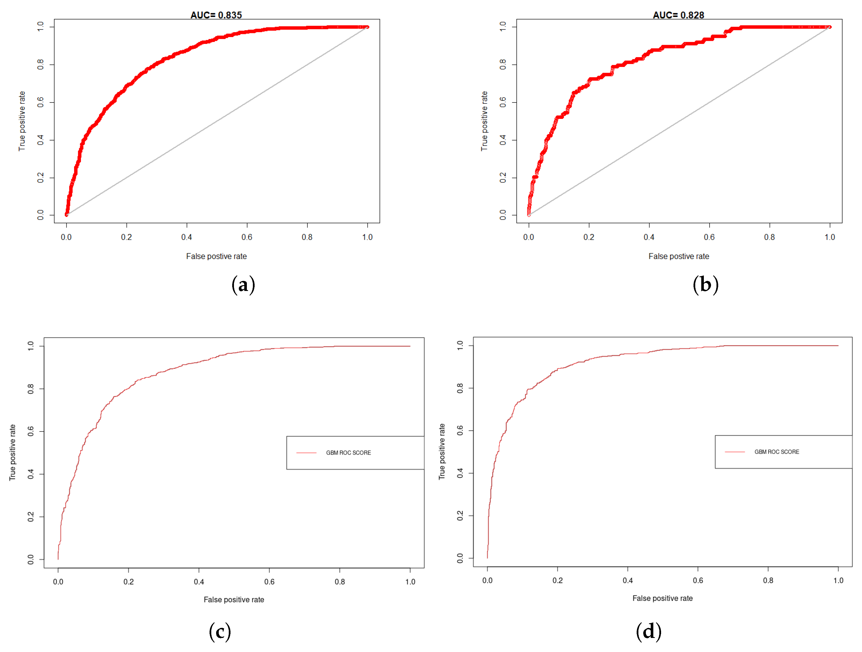
It is essential to know the relative contribution of each predictor in a model and the model’s accuracy. Table 2 presents model assessment indices measured by AUC, PPP, Cohen’s κ and spec_sen. First, we used the AUC values to identify and check the accuracy of the MaxEnt and BRT models. (Table 2 and Figure A3) present the results of the AUC values for the MaxEnt and BRT models for BTD and IBR. The results show that the AUC values for MaxEnt and BRT were >0.5, implying that both models have good accuracy. However, the AUC values for BRT models were higher than those of MaxEnt. The range of values of agreement for the kappa statistics were good (>0.4) except for the MaxEnt models in the training set. The PPP values also indicate the goodness of the predicted results.
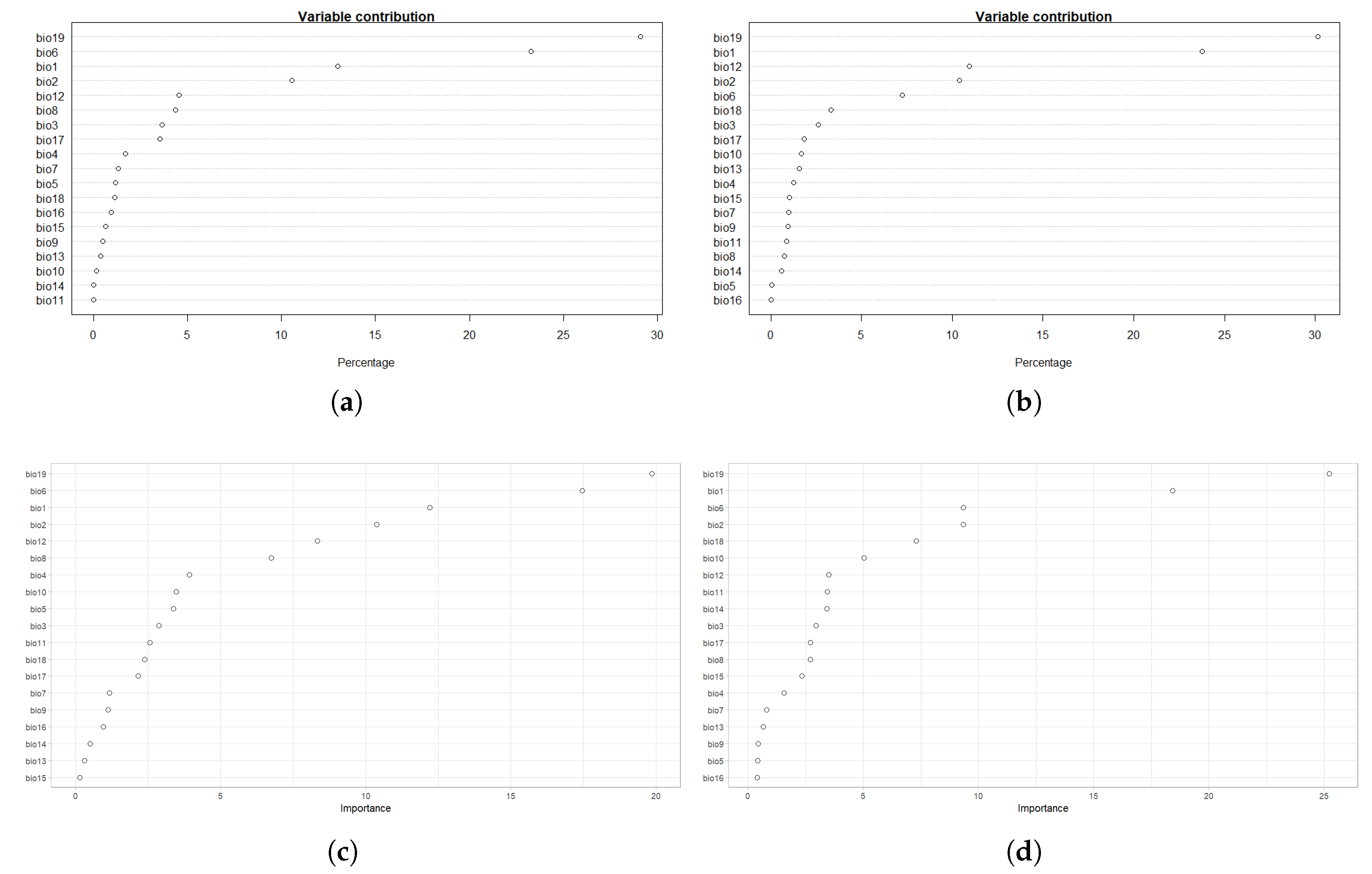
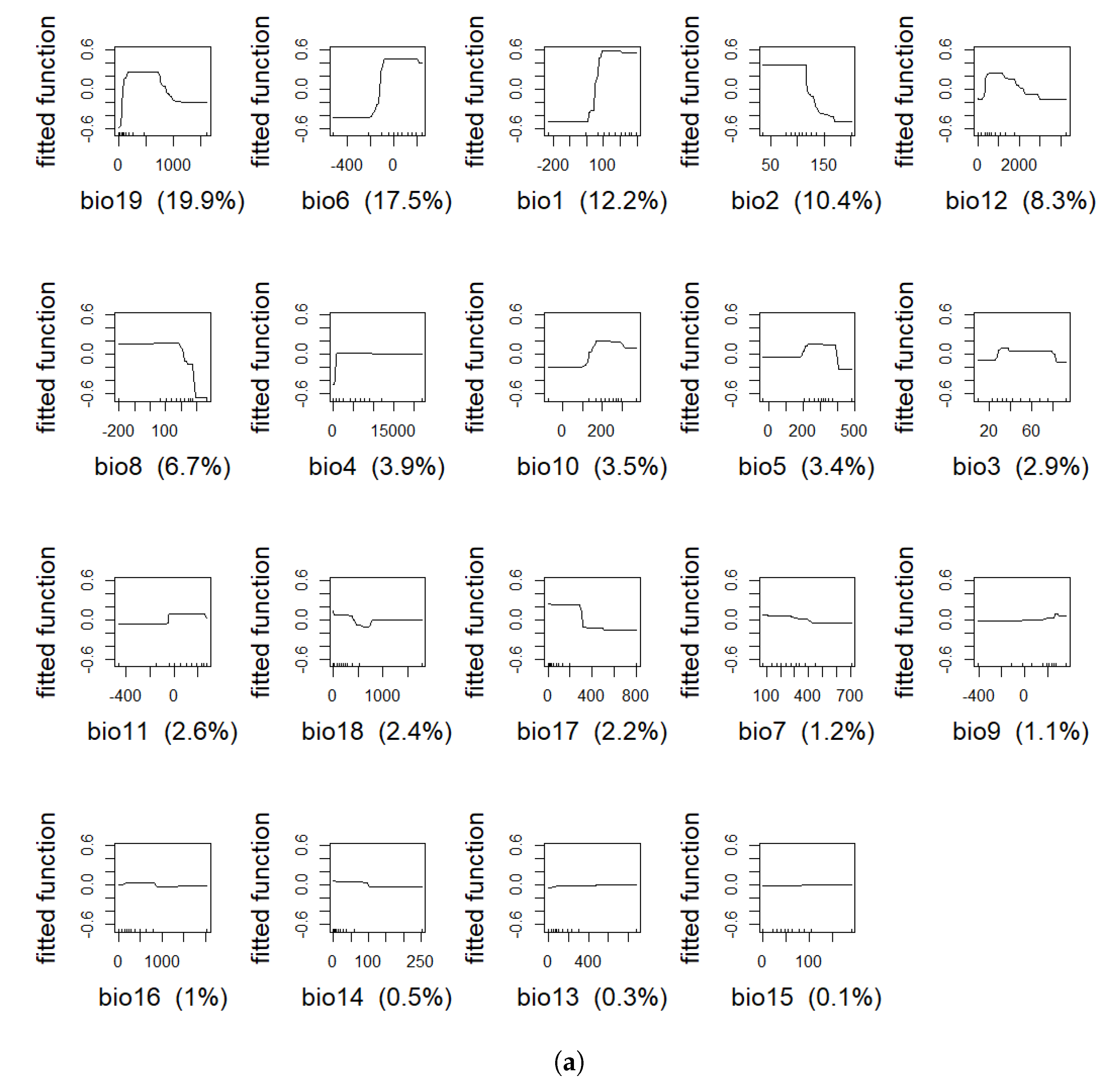
Table 3 and Figure A2 present the relative importance of each of the 19 predictors in the model. We measured the contribution of each variable to the habitat suitability index. The magnitude of the contribution is presented as percentages and indicates how much the variable is influential in driving the probability of occurrence of BRD. The six variables with the highest relative importance for BTQ were the precipitation of the coldest quarter (bio19), minimum temperature of the coldest month (bio6), annual mean temperature (bio1), mean diurnal range (bio2), annual precipitation (bio12) and mean temperature of the wettest quarter (bio8). These variables accounted for 75% of the drivers of BTD. Similar relative importance variables were observed for IBR, except for the addition of the mean temperature of the warmest quarter (bio10) and precipitation of the warmest quarter (bio18).
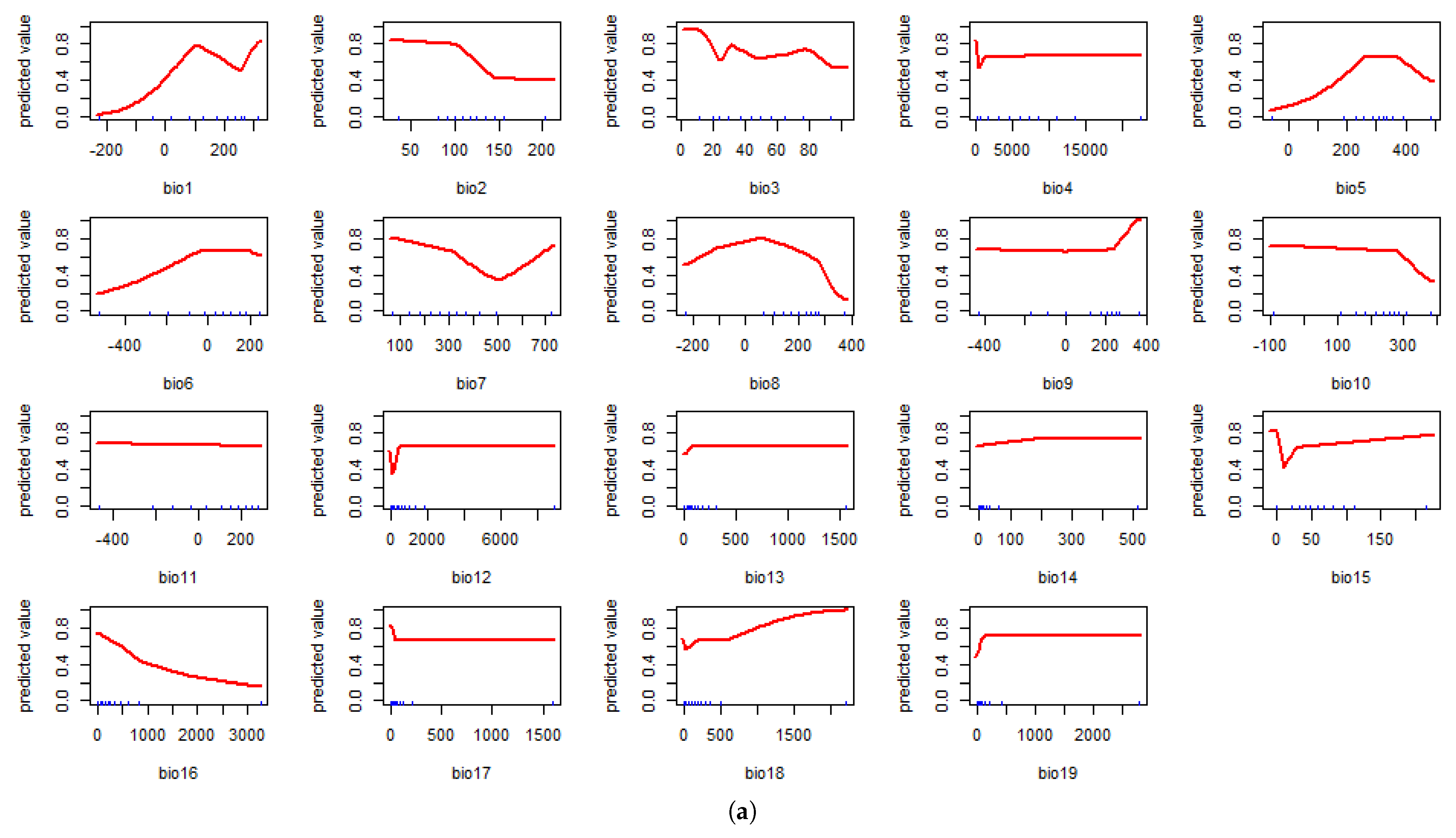
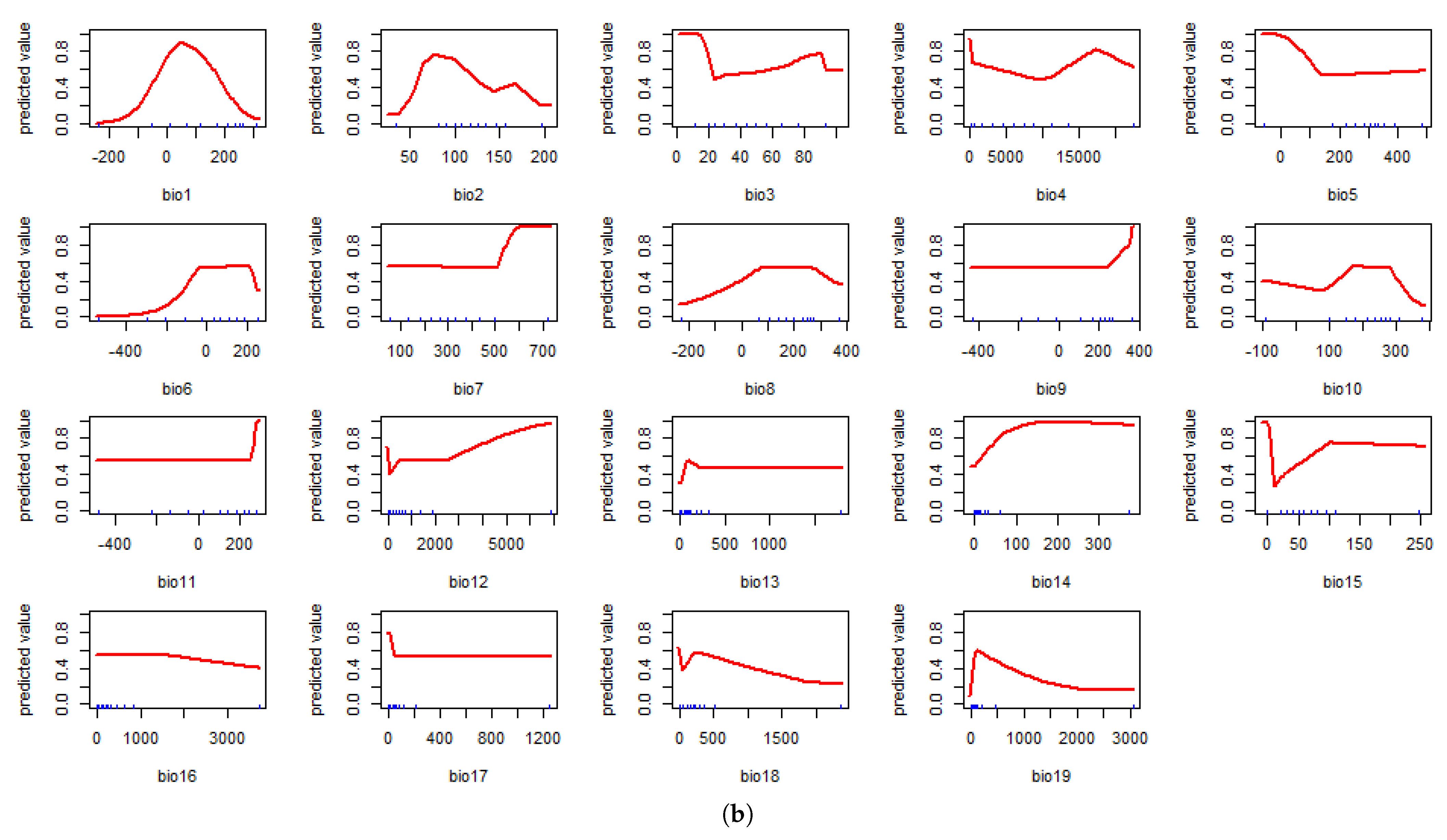
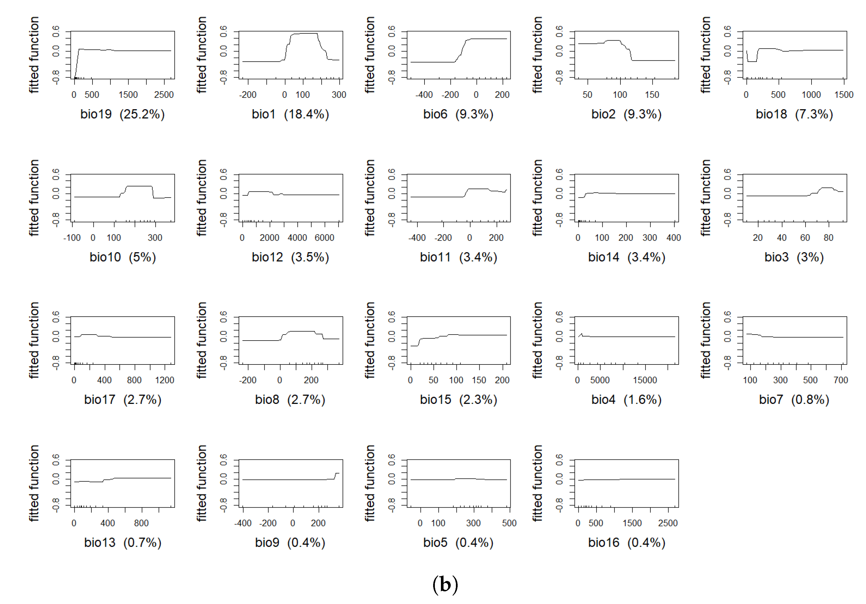
In addition to the AUC and variable importance, we used the ecological response curve to visualise the marginal effect from ME and BRT SDMS (Figure A1 and Figure A4). The figures indicate the predicted probability of the presence of BRD on the y-axis and the scaled value for the predictors (×10). These response curves provide more insight into the predictors than do the variable contributions.
For example, consider the top panel of Figure A1 presenting the response curves for the ME model for BTB. We observed that, below the threshold of −10 °C of bio1, the probability for BTD occurrence is near zero and then increases non-linearly up to 30 °C. This implies that the BTD habitat suitability ranges from an annual mean temperature of −10 °C to 30 °C.
For bio2 (the mean diurnal range), which is the mean of the difference between the monthly maximum temperature and minimum temperature, we saw that a value higher than 4 °C decreased the probability of BTD occurrence. Bio8, on the other hand, revealed an inverse U-shape between the mean temperature of the wettest quarter and the risk of BTD occurrence. The relationship between IBR and the predictors is depicted in the bottom panel of Figure A1. For example, the relationship between bio1 and IBR was bell-shaped with the least favourable threshold of annual mean temperature <−20 °C and >30 °C.
For BRT (Figure A4), we observed that bio6, in addition to bio19, bio12, bio8, bio1 and bio2 had the highest variable contribution for the likelihood of the occurrence of BTD. Looking at bio6, the minimum temperature of the coldest month, below the threshold of −20 °C, reduced the likelihood of BRD to zero and then increased non-linearly up −10 °C and, thereafter, became constant. This implies that the BTD likelihood occurrence increases with a minimum temperature ranging between −20 °C and −10 °C.
Similarly, for IBR (bottom panel Figure A4), bio2, in addition to bio19, bio6, bio1 and bio18, had the highest variable contribution for the suitable habitat for IBR. For bio2, we observe that, below the threshold of 6 °C, the likelihood for IBR occurrence was zero and then non-linearly increased up to 10 °C and then decreased again.

4.2. Predicted Suitability

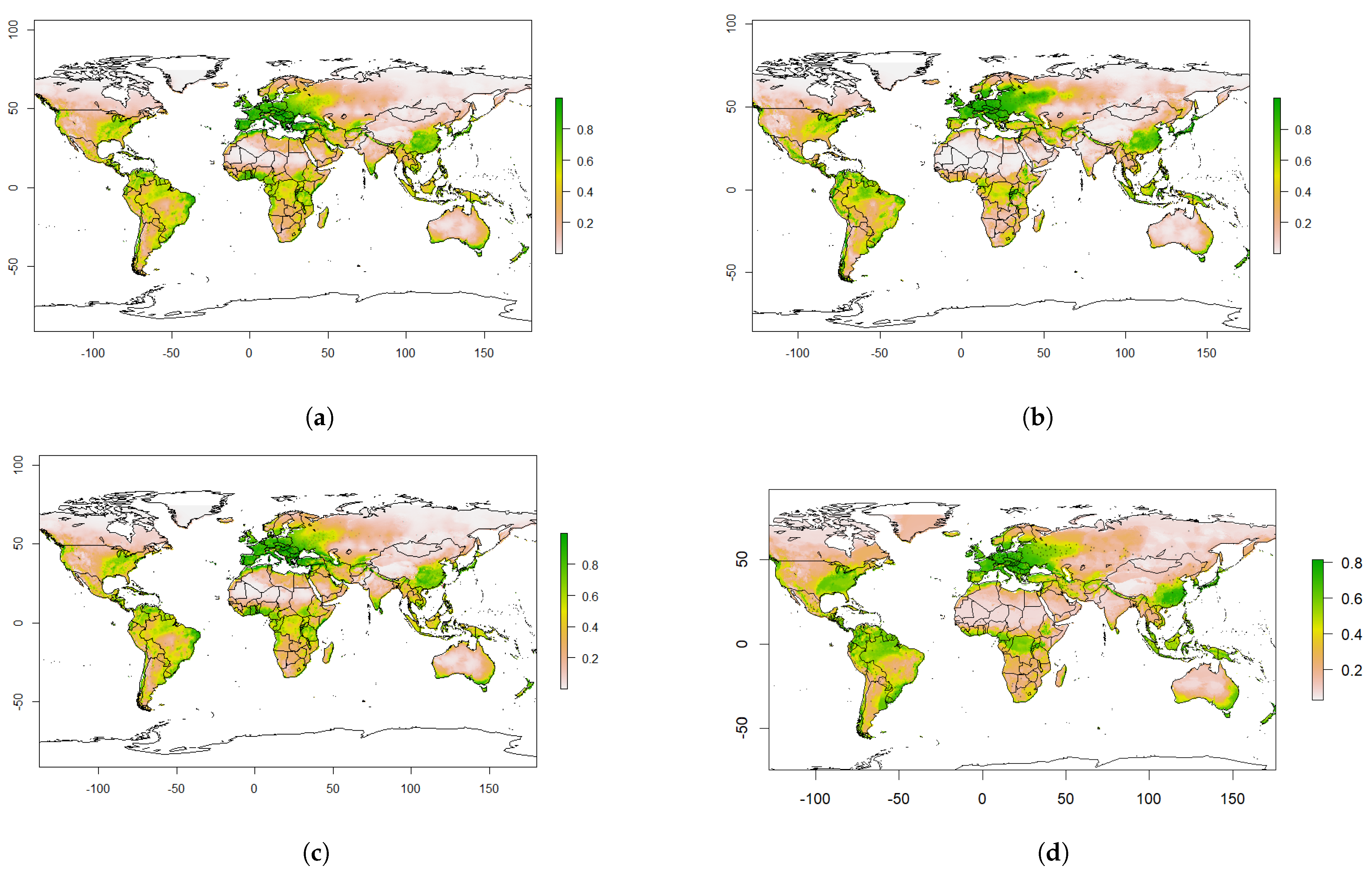
Figure 2 presents the distribution of habitat suitability index for BTD and IBR using climate variables described in Table 1. The predicted values represent the probabilities for suitable habitat for BRD occurrence, and they range from 0 to 1. The results from ME (Figure 2 top panel) and BRT (Figure 2 bottom panel) predicted similar geographically favourable habitats for BTD and IBR. The distribution of favourable habitats for BTD was mostly Europe, western Russia, southern China, Australia and India, central, western and eastern parts of Africa, South America and North America. While the results from ME and BRT were similar, ME included some areas in Africa and South America suitable for BTD. IBR, on the other hand, had a wider geographically suitable habitat, including Europe, western Russia, southern China, America and central Africa. Prediction for habitat suitability for IBR was similar for both models.

4.3. Predicted Future Suitability

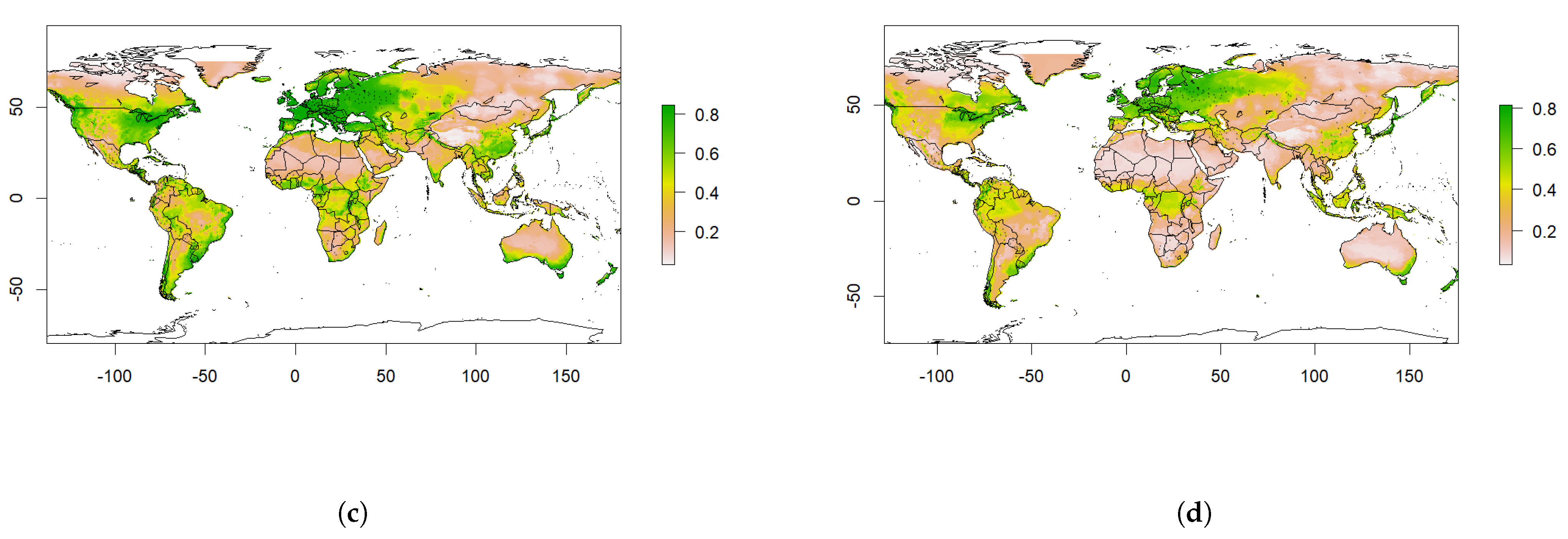
The future (2021–2040) predictions of habitat suitability for BTD and IBR occurrences using ME and BRT are presented in the top and bottom panels of Figure 3, respectively. Compared to the current geographical distribution of habitat suitable for BTD and IBR described above, we observed that the geographical spread of favourable habitat for BTD and IBR extended to western Russia, North America and the Middle East in Figure 3.

4.4. The Effect of Climate Change

Furthermore, we examined the effects of climate change on the suitability of habitat of BRD for ME. The differences in the suitability habitat index between the current time and the future are shown in Figure 4. Positive values indicate an increasing spread of favourable habitat conditions for BRD, while negative values indicate a reduction in favourable habitat conditions. Greener colours indicate a change in habitat suitability, yellow colours indicate no change, and brownish colours indicate a reduction in habitat suitability for BRD. From Figure 4, we observed that many changes in suitability were made in northern Russia, North America, Finland, Sweden, Saudi Arabia and northern and central Africa.

5. Discussion

This study extended previous research in several important ways in advancing our understanding of the BRD emergence or re-emergence and the interaction between BRD and climate factors. Using two machine-learning modelling techniques (BRT and MaxEnt) to analyse complex ecological data, we identified the effect of spatial and climate drivers on the emergence and spread of BRD. The results generated a novel description of the global suitability index of BRD prevalence.
The applied focus of this study to deliver global risk maps of emerging or re-emerging of BRDs supports targeted improvements in biosecurity surveillance. The study used advanced statistical models to explain the unequal global distribution of occurrence, event detection and surveillance using an algorithm-driven approach to obtain a realistic mapping of the reporting incidence of BRD even on smaller country-scale resolutions. This allowed us to estimate and predict the risk of concentration of BRDs at a given location with biological and bioclimatic variables. Consequently, this study provides policymakers and farmers with a better understanding of the impacts and risks of climate change on livestock.
The findings of this study showed that a favourable habitat for BRD occurrence is associated with the mean annual temperature, precipitation of the coldest quarter, mean diurnal range and minimum temperature of the coldest month. These variables may represent the same mechanism as tropical regions are generally areas with high biodiversity [34]. However, the predicted suitability maps showed that western and central Africa have favourable habitats for the occurrence of BRD, making it a cold and wet area, which is a contradiction since it is known that western and central Africa are hot areas.
Consistent with this study, Cusack and colleagues [35] found an association between the minimum daily temperature and BRD occurrence in Australian feedlots. Furthermore, as shown by the response curves for MaxEntand BRT, a threshold above the minimum temperature of the coldest month, −20 °C, increases the probability of BRD occurrence. This explains why the incidence of BRD is concentrated in regions in Europe, America and Russia.
The precipitation of the coldest quarter is an important climate variable to consider when evaluating the risk of respiratory infections, such as BRD. From a mechanistic perspective, precipitation can directly impact the environment where cattle are housed by creating damp and muddy conditions, which can increase the risk of respiratory infections and thermal stress [36]. Precipitation patterns can influence the transmission of respiratory pathogens [37] by dispersing pathogen-laden respiratory secretions and washing away protective mucus from the respiratory tracts of cattle, making them more susceptible to infection.
Additionally, high precipitation levels can also lead to waterlogged feed, reducing its quality via contaminants, weakening the immune system and increasing the risk of respiratory diseases [36,38,39,40]. By understanding the impacts of precipitation on the environment, feed availability and pathogen transmission, more effective strategies can be implemented to reduce the risk of bovine respiratory diseases.
This study is not with limitations. First, the SDMs only showed how similar locations might in relation to the covariates included in the analysis and other locations where BRD was previously found [41]; they do not predict the extent/magnitude of BRD infection. More so, the SDMs do not provide information on the animal’s condition but only identify suitable habitats for the occurrence of BRD. As MaxEnt and BRT best predict the average environmental habitat suitability for BRD incidence, the suitable habitats are the regions with an average estimate exceeding the optimal threshold, such as Europe and western Russia.
Secondly, there is also a possibility that the two models can predict high environmental suitability among regions similar to regions that are BRD endemic, even if the regions contain no BRD infections. This makes the covariates determining high environmental suitability biased towards regions with high BRD prevalence. Finally, it is not always effective to capture a particular ecological niche using a 5 × 5 km resolution of covariate patterns for all the locations, as sometimes the vector might travel beyond the range of 5 km [42].

6. Conclusions

In summary, the use of climate-based SDMs to predict potential species ranges were shown to provide a powerful predictive power. This study presented the first attempt to use BRT and MaxEnt to identify favourable habitats for the occurrence of BRD. Information gathered from such SDMs can be used to alert governments and conservation organisations about the possibility of BRD being established in their respective regions. The results showed that BRT was the best model to predict the favourable habitat for BRD occurrence with an AUC value higher than MaxEnt. BRD-free areas that were identified as suitable could be investigated in early detection and control to prevent the formation of species. The methods used here can also be used in the prediction of other invasive species.

Author Contributions

Conceptualization, J.K.G. and O.A.A.; methodology, J.K.G. and O.A.A.; software, J.K.G. and M.A.D.; validation, M.A.D., J.-P.N.N., A.P., J.O., F.E. and O.A.A.; formal analysis, J.K.G.; investigation, J.K.G., M.A.D., A.P., J.O., F.E. and O.A.A.; data curation, J.K.G. and O.A.A.; writing—original draft preparation, J.K.G.; writing—review and editing, J.K.G., J.-P.N.N., M.A.D., A.P., J.O., F.E. and O.A.A.; visualization, J.K.G.; supervision, O.A.A. All authors have read and agreed to the published version of the manuscript.

Funding

This research received no external funding.

Institutional Review Board Statement

Not applicable.

Data Availability Statement

This study was based on publicly available data sets. The occurrence data on BRD was obtained from the World Organisation for Animal Health’s World Animal Health Information System, and the BioClimate data were extracted from Bio-ORACLE.

Acknowledgments

Open Access funding provided by the Qatar National Library.

Conflicts of Interest

The authors declare no conflict of interest.

Appendix A

Figure A1. Response curves for the 19 predictors for ME. (a) BTD data and (b) IBR data. The y-axis presents the predicted probability of the presence of IBR, and the scaled value for the predictors is presented on the x-axis (×10).
Mathematics 11 01354 g0a1aMathematics 11 01354 g0a1b
Figure A2. Variable importance indicating the contribution (%) of each predictor to the models. Full models (a,c) and reduced models (b,d) for BT and IBR, respectively.
Mathematics 11 01354 g0a2
Figure A3. ROC curves for BTD and IBR from ME and BRT at different thresholds. (a,b) The ROC curves for BTD and IBR, respectively, from ME. (c,d) The ROC curves for BTD and IBR, respectively, from BRT.
Mathematics 11 01354 g0a3
Figure A4. Response curves for the 19 predictors for BRT. (a) BTD data and (b) IBR data. The y-axis presents the predicted probability of the presence of BRD, and the scaled value for the predictors is presented on the x-axis (×10).
Mathematics 11 01354 g0a4aMathematics 11 01354 g0a4b

References

  1. Fulton, R.W. Bovine respiratory disease research (1983–2009). Anim. Health Res. Rev. 2009, 10, 131–139. [Google Scholar] [CrossRef] [PubMed]
  2. Fernández, M.; Ferreras, M.d.C.; Giráldez, F.J.; Benavides, J.; Pérez, V. Production Significance of Bovine Respiratory Disease Lesions in Slaughtered Beef Cattle. Animals 2020, 10, 1770. [Google Scholar] [CrossRef]
  3. Taylor, J.D.; Fulton, R.W.; Lehenbauer, T.W.; Step, D.L.; Confer, A.W. The epidemiology of bovine respiratory disease: What is the evidence for preventive measures? Can. Vet. J. 2010, 51, 1351. [Google Scholar]
  4. Johnson, K.K.; Pendell, D.L. Market impacts of reducing the prevalence of bovine respiratory disease in United States beef cattle feedlots. Front. Vet. Sci. 2017, 4, 189. [Google Scholar] [CrossRef] [PubMed] [Green Version]
  5. Booker, C.W.; Abutarbush, S.M.; Morley, P.S.; Jim, G.K.; Pittman, T.J.; Schunicht, O.C.; Perrett, T.; Wildman, B.K.; Fenton, R.K.; Guichon, P.T.; et al. Microbiological and histopathological findings in cases of fatal bovine respiratory disease of feedlot cattle in western Canada. Can. Vet. J. 2008, 49, 473. [Google Scholar] [PubMed]
  6. Fentie, T.; Guta, S.; Mekonen, G.; Temesgen, W.; Melaku, A.; Asefa, G.; Tesfaye, S.; Niguse, A.; Abera, B.; Kflewahd, F.Z.; et al. Assessment of major causes of calf mortality in urban and periurban dairy production system of Ethiopia. Vet. Med. Int. 2020, 2020, 3075429. [Google Scholar] [CrossRef] [PubMed] [Green Version]
  7. Jimmy, J.; Sones, K.; Grace, D.; MacMillan, S.; Tarawali, S.; Herrero, M. Beyond milk, meat, and eggs: Role of livestock in food and nutrition security. Anim. Front. 2013, 3, 6–13. [Google Scholar]
  8. Thornton, P.; Herrero, M. The Inter-Linkages Between Rapid Growth in Livestock Production, Climate Change, and the Impacts on Water Resources, Land Use, and Deforestation; World Bank Policy Research Working Paper, (5178); Elsevier: Amsterdam, The Netherlands, 2010. [Google Scholar]
  9. Thornton, P.K.; Gerber, P.J. Climate change and the growth of the livestock sector in developing countries. Mitig. Adapt. Strateg. Glob. Chang. 2010, 15, 169–184. [Google Scholar] [CrossRef]
  10. Herrero, M.; Petr, H.; John, M.; Amanda, P.; Hugo, V. African Livestock Futures: Realizing the Potential of Livestock for Food Security, Poverty Reduction and the Environment in Sub-Saharan Africa; Office of the Special Representative of the UN Secretary General for Food Security and Nutrition and the United Nations System Influenza Coordination (UNSIC): Geneva, Switzerland, 2014; Available online: https://pure.iiasa.ac.at/id/eprint/11154/1/LiveStock_Report_ENG_20140725_02_web%282%29.pdf (accessed on 27 November 2022).
  11. Sarchet, J.J.; Pollreisz, J.P.; Bechtol, D.T.; Blanding, M.R.; Saltman, R.L.; Taube, P.C. Limitations of bacterial culture, viral PCR, and tulathromycin susceptibility from upper respiratory tract samples in predicting clinical outcome of tulathromycin control or treatment of bovine respiratory disease in high-risk feeder heifers. PLoS ONE 2022, 17, E0247213. [Google Scholar] [CrossRef]
  12. Hay, S.I.; Battle, K.E.; Pigott, D.M.; Smith, D.L.; Moyes, C.L.; Bhatt, S.; Brownstein, J.S.; Collier, N.; Myers, M.F.; Geoge, D.B.; et al. Global mapping of infectious disease. Philos. Trans. R. Soc. Biol. Sci. 2013, 368, 20120250. [Google Scholar] [CrossRef]
  13. Liu, Z.; Peng, C.; Work, T.; Candau, J.-N.; DesRochers, A.; Kneeshaw, D. Application of machine-learning methods in forest ecology: Recent progress and future challenges. Environ. Rev. 2018, 26, 339–350. [Google Scholar] [CrossRef] [Green Version]
  14. Aertsen, W.; Kint, V.; Van Orshoven, J.; Özkan, K.; Muys, B. Comparison and ranking of different modelling techniques for prediction of site index in Mediterranean mountain forests. Ecol. Model. 2010, 221, 1119–1130. [Google Scholar] [CrossRef]
  15. Franklin, J. Species distribution models in conservation biogeography: Developments and challenges. Divers. Distrib. 2013, 19, 1217–1223. [Google Scholar] [CrossRef]
  16. Elith, J.; John, R.L. Species distribution models: Ecological explanation and prediction across space and time. Annu. Rev. Ecol. Evol. Syst. 2009, 40, 677–697. [Google Scholar] [CrossRef]
  17. Naimi, B.; Hamm, N.A.S.; Groen, T.A.; Skidmore, A.K.; Toxopeus, A.G. Where is positional uncertainty a problem for species distribution modelling? Ecography 2014, 37, 191–203. [Google Scholar] [CrossRef]
  18. Fick, S.E.; Hijman, R.J. WorldClim 2: New 1-km spatial resolution climate surfaces for global land areas. Int. J. Climatol. 2017, 37, 4302–4315. [Google Scholar] [CrossRef]
  19. Harris, I.P.D.J.; Jones, P.D.; Osborn, T.J.; Lister, D.H. Updated high-resolution grids of monthly climatic observations—The CRU TS3. 10 Dataset. Int. J. Climatol. 2014, 34, 623–642. [Google Scholar] [CrossRef] [Green Version]
  20. Tyberghein, L.; Verbruggen, H.; Pauly, K.; Troupin, C.; Mineur, F.; De Clerck, O. Bio-ORACLE: A global environmental dataset for marine species distribution modelling. Glob. Ecol. Biogeogr. 2012, 21, 272–281. [Google Scholar] [CrossRef]
  21. Baldwin, R.A. Use of maximum entropy modeling in wildlife research. Entropy 2009, 11, 854–866. [Google Scholar] [CrossRef]
  22. Phillips, S.J.; Anderson, R.P.; Schapire, R.E. Maximum entropy modeling of species geographic distributions. Ecol. Model. 2006, 190, 231–259. [Google Scholar] [CrossRef] [Green Version]
  23. Adegboye, O.A.; Adegboye, M. Spatially correlated time series and ecological niche analysis of cutaneous leishmaniasis in Afghanistan. Int. J. Environ. Res. Public Health 2017, 14, 309. [Google Scholar] [CrossRef] [PubMed] [Green Version]
  24. Adegboye, O.A.; Kotze, D. Epidemiological analysis of spatially misaligned data: A case of highly pathogenic avian influenza virus outbreak in Nigeria. Epidemiol. Infect. 2014, 142, 940–949. [Google Scholar] [CrossRef] [PubMed] [Green Version]
  25. Grendár, M., Jr.; Grendár, M. Maximum entropy: Clearing up mysteries. Entropy 2001, 3, 58–63. [Google Scholar] [CrossRef] [Green Version]
  26. Peterson, A.T.; Soberón, J.; Pearson, R.G.; Anderson, R.P.; Martínez-Meyer, E.; Nakamura, M.; Araújo, M.B. Ecological niches and geographic distributions (MPB-49). In Ecological Niches and Geographic Distributions (MPB-49); Princeton University Press: Princeton, NJ, USA, 2011. [Google Scholar]
  27. Shannon, C.E. The Best Detection of PulsesBell Laboratories Memorandum, June 22, 1944; Wiley-IEEE Press: Hoboken, NJ, USA, 1993; pp. 148–150. [Google Scholar]
  28. Shannon, C.E. A mathematical theory of communication. Bell Syst. Tech. J. 1948, 27, 379–423. [Google Scholar] [CrossRef] [Green Version]
  29. Dudík, M.; Phillips, S.; Schapire, R.E. Correcting sample selection bias in maximum entropy density estimation. In Advances in Neural Information Processing Systems; Princeton University Press: Princeton, NJ, USA, 2005; p. 18. [Google Scholar]
  30. Fielding, A.H.; Bel, J.F. A review of methods for the assessment of prediction errors in conservation presence/absence models. Environ. Conserv. 1997, 24, 38–49. [Google Scholar] [CrossRef]
  31. Grömping, U. Variable importance assessment in regression: Linear regression versus random forest. Am. Stat. 2009, 63, 308–319. [Google Scholar] [CrossRef]
  32. Phillips, S.J.; Anderson, R.P.; Dudík, M.; Schapire, R.E.; Blair, M.E. Opening the black box: An open-source release of Maxent. Ecography 2017, 40, 887–893. [Google Scholar] [CrossRef]
  33. Elith, J.; Leathwick, J.R.; Hastie, T. A working guide to boosted regression trees. J. Anim. Ecol. 2008, 77, 802–813. [Google Scholar] [CrossRef]
  34. Mittermeier, R.A.; Myers, N.; Mittermeier, C.G.; Gil, P.R. Hotspots: Earth’s Biologically Richest and Most Endangered Terrestrial Ecoregions; CEMEX, SA, Agrupación Sierra Madre, SC: Mexico City, Mexico, 1999. [Google Scholar]
  35. Cusack, P.M.V.; McMeniman, N.P.; Lean, I.J. Feedlot entry characteristics and climate: Their relationship with cattle growth rate, bovine respiratory disease and mortality. Aust. Vet. J. 2007, 85, 311–316. [Google Scholar] [CrossRef]
  36. Robertson, J. Cattle housing: Design and management. In Bovine Medicine; John Wiley & Sons, Inc.: Hoboken, NJ, USA, 2015; pp. 517–524. [Google Scholar]
  37. Leung, N.H.L. Transmissibility and transmission of respiratory viruses. Nat. Rev. Microbiol. 2021, 19, 528–545. [Google Scholar] [CrossRef]
  38. Kuddus, M.A.; McBryde, E.S.; Adegboye, O.A. Delay effect and burden of weather-related tuberculosis cases in Rajshahi province, Bangladesh, 2007–2012. Sci. Rep. 2019, 9, 12720. [Google Scholar] [CrossRef] [Green Version]
  39. Adegboye, O.A.; McBryde, E.S.; Eisen, D.P. Epidemiological analysis of association between lagged meteorological variables and pneumonia in wet-dry tropical North Australia, 2006–2016. J. Expo. Sci. Environ. Epidemiol. 2020, 30, 448–458. [Google Scholar] [CrossRef] [PubMed]
  40. Alegbeleye, O.O.; Sant’Ana, A.S. Manure-borne pathogens as an important source of water contamination: An update on the dynamics of pathogen survival/transport as well as practical risk mitigation strategies. Int. J. Hyg. Environ. Health 2020, 227, 113524. [Google Scholar] [CrossRef] [PubMed]
  41. Barbet-Massin, M.; Jiguet, F.; Albert, C.H.; Thuiller, W. Selecting pseudo-absences for species distribution models: How, where and how many? Methods Ecol. Evol. 2012, 3, 327–338. [Google Scholar] [CrossRef]
  42. Jacob, B.G.; Novak, R.J.; Toe, L.D.; Sanfo, M.; Griffith, D.A.; Lakwo, T.L.; Habomugisha, P.; Katabarwa, M.N.; Unnasch, T.R. Validation of a remote sensing model to identify Simulium damnosum sl breeding sites in sub-Saharan Africa. PLoS Negl. Trop. Dis. 2013, 7, E2342. [Google Scholar] [CrossRef] [PubMed]
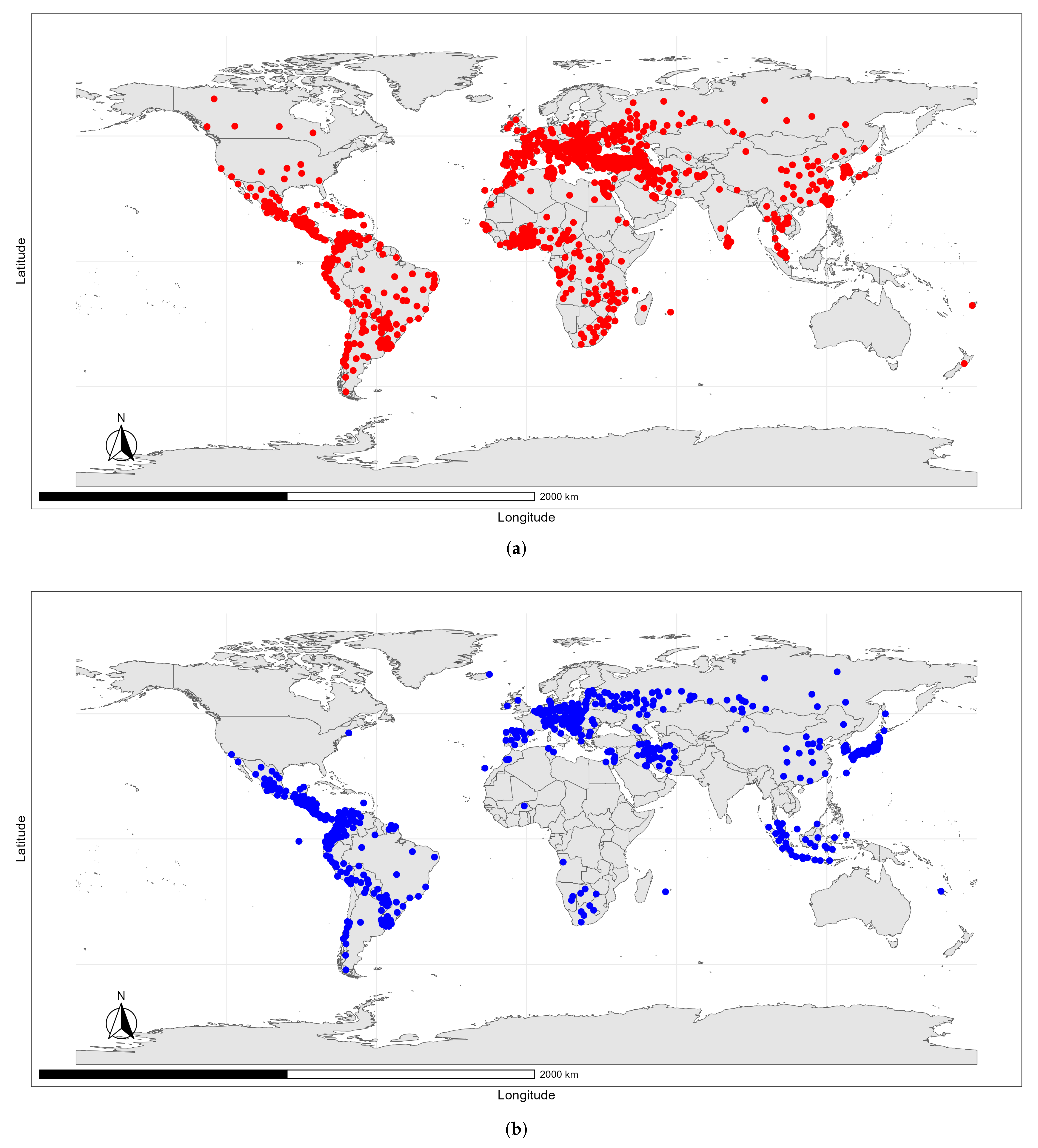
Figure 1. Global distribution of BRD: (a) the red dots show the occurrence of Bovine Tuberculosis Disease (BTD) and (b) the blue dots represent the occurrence of Infectious Bovine Rhinotracheitis (IBR).
Mathematics 11 01354 g001
Figure 2. Prediction of habitat suitability distribution for (a,b) BTD and IBR, respectively, using ME. (c,d) BTD and IBR, respectively, using BRT. The greenish colour in the scale colour bar indicates suitable habitats for BRD occurrence, while the pinkish colour indicates habitats that are less suitable for BRD occurrence.
Mathematics 11 01354 g002
Figure 3. Future prediction of habitat suitability distribution for BRD using ME and BRT. (a,b) BTD and IBR, respectively, using ME. (c,d) BTD and IBR, respectively, using BRT. The greenish colour in the scale colour bar indicates suitable habitats for BRD occurrence, while the pinkish colour indicates habitats that are less suitable for BRD occurrence.
Mathematics 11 01354 g003aMathematics 11 01354 g003b
Figure 4. Changes in habitat suitability for (a) BTB and (b) IBR.
Mathematics 11 01354 g004
Table 1. Bioclimatic variables used in this study.
AcronymDescriptionUnit
bio1Annual Mean Temperature°C
bio2Mean Diurnal Range (Mean of monthly (maximum temperature–minimum temperature))°C
bio3Isothermality (BIO2/BIO7) ( × 100 ) °C
bio4Temperature Seasonality (SD × 100 )%
bio5Max Temperature of Warmest Month°C
bio6Min Temperature of Coldest Month°C
bio7Temperature Annual Range (BIO5-BIO6)°C
bio8Mean Temperature of Wettest Quarter°C
bio9Mean Temperature of Driest Quarter°C
bio10Mean Temperature of Warmest Quarter°C
bio11Mean Temperature of Coldest Quarter°C
bio12Annual Precipitationmm
bio13Precipitation of Wettest Monthmm
bio14Precipitation of Driest Monthmm
bio15Precipitation Seasonality (CV)%
bio16Precipitation of Wettest Quartermm
bio17Precipitation of Driest Quartermm
bio18Precipitation of Warmest Quartermm
bio19Precipitation of Coldest Quartermm
Note: Standard Deviation (SD) and Coefficient of Variation (CV).
Table 2. Assessment of model accuracy for predicting the global area under the curve (AUC) of a receiver operator curve (AUC), positive predictive power (PPP), Cohen’s kappa and the threshold at which the sum of the sensitivity (true positive rate) and specificity (true negative rate) is highest (spec_sens).
ModelBRDTrainingTest
AUCPPPKappaSens_Spec.AUCPPPKappaSens_Spec.
MaxEntBTD0.8350.7250.3770.4110.9100.6440.2850.340
IBR0.8280.5730.3780.4150.8830.6160.3010.281
BRTBTD0.8780.7920.4560.4020.9360.6030.5110.512
IBR0.9160.7230.5160.3950.8740.8330.4750.423
Table 3. Variable relative importance for the BRT model.
Variable% BTD% IBR
bio1919.925.2
bio617.59.3
bio112.218.4
bio210.49.3
bio128.33.5
bio86.72.7
bio43.91.6
bio103.55.0
bio53.40.4
bio32.93.0
bio112.63.4
bio182.47.3
bio172.22.7
bio71.20.8
bio91.10.4
bio1610.4
bio140.53.4
bio130.30.7
bio150.12.3
Note: Variables are described in Table 1.
Disclaimer/Publisher’s Note: The statements, opinions and data contained in all publications are solely those of the individual author(s) and contributor(s) and not of MDPI and/or the editor(s). MDPI and/or the editor(s) disclaim responsibility for any injury to people or property resulting from any ideas, methods, instructions or products referred to in the content.