
Multi-Objective Optimization for Mixed-Model Two-Sided Disassembly Line Balancing Problem Considering Partial Destructive Mode


Abstract
1. Introduction
2. Problem Statement
2.1. Problem Description
2.2. Mathematical Model
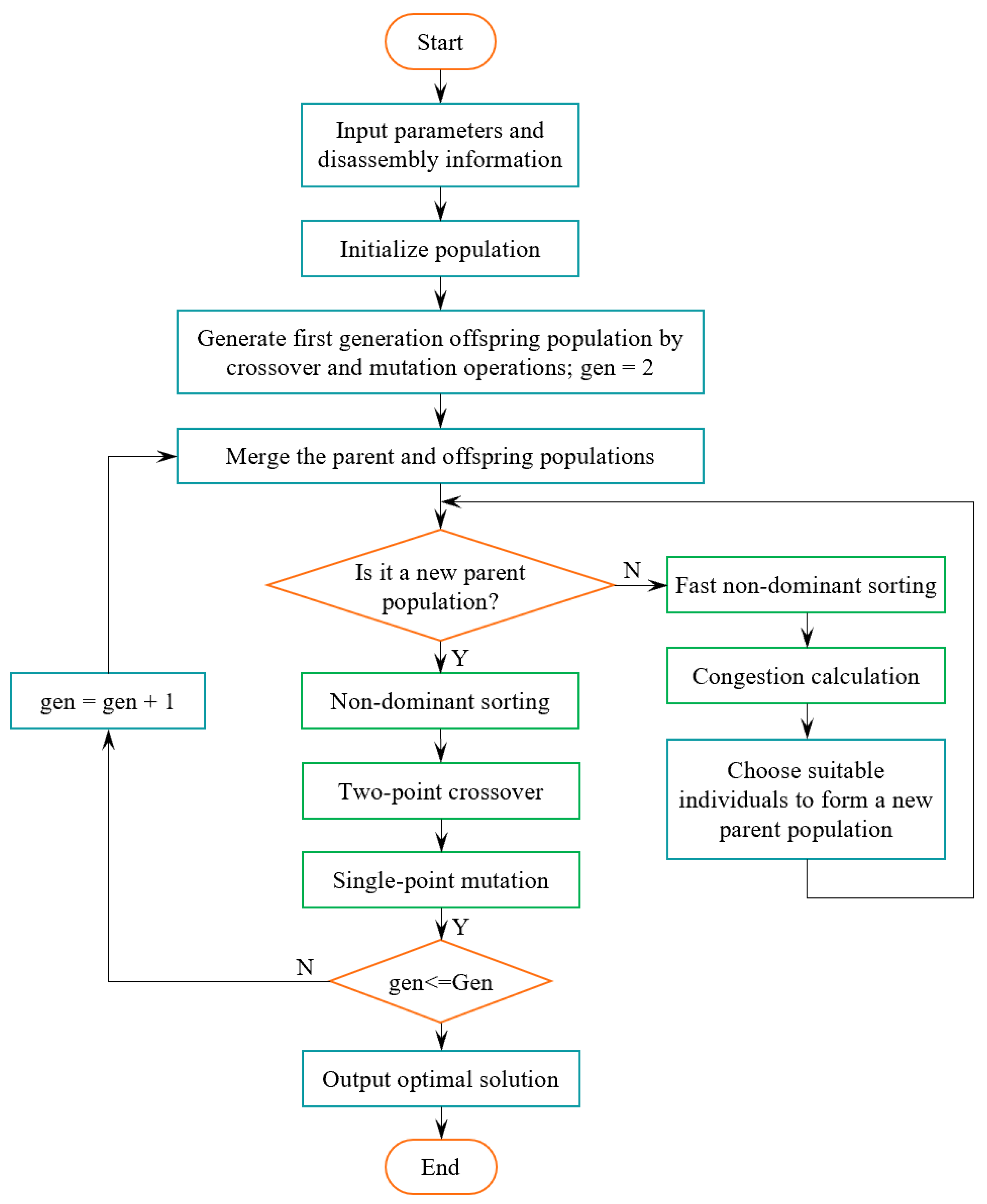
3. The Proposed Method
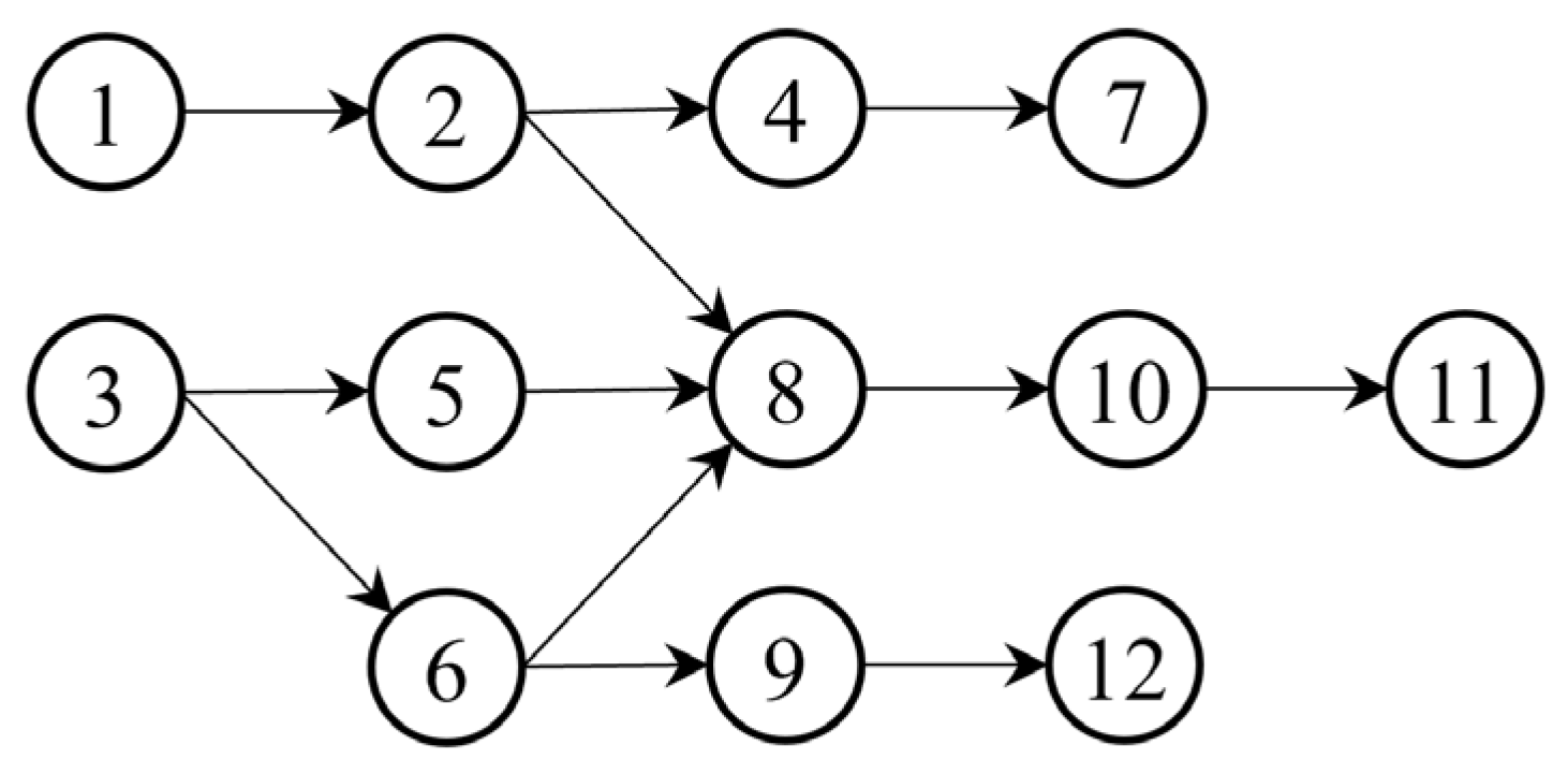
3.1. Encoding
3.2. Decoding
3.3. Crossover
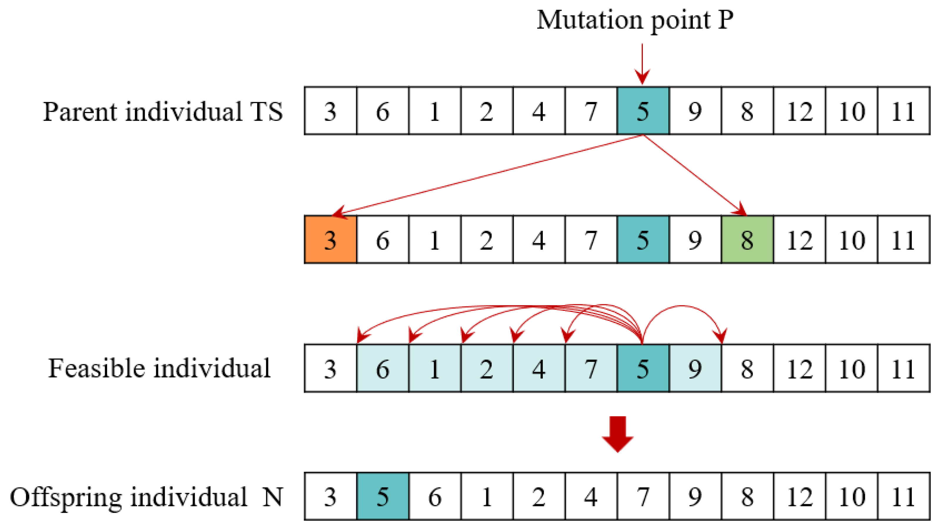
3.4. Mutation
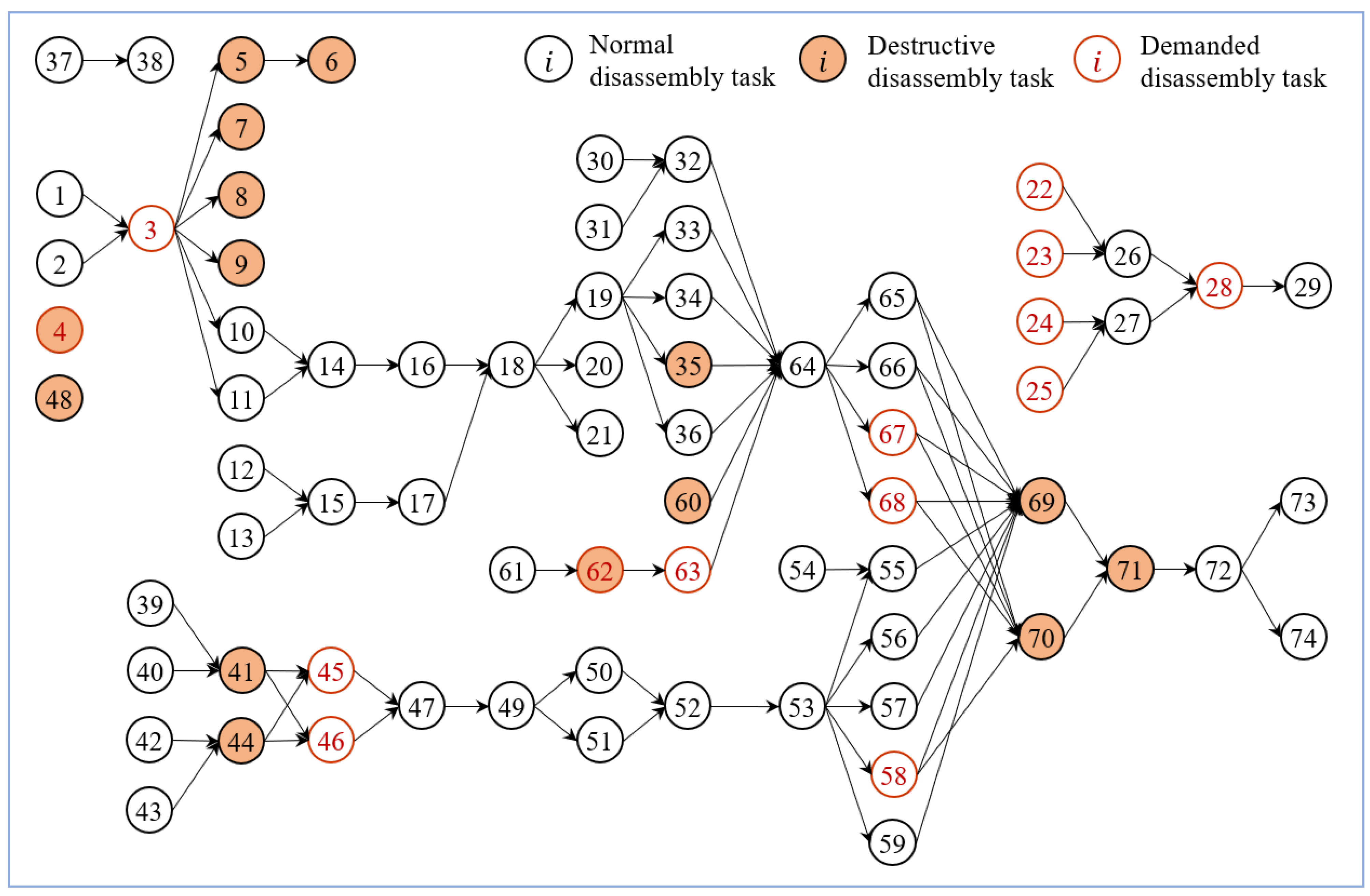
4. Case Study
5. Conclusions
Author Contributions
Funding
Data Availability Statement
Conflicts of Interest
Appendix A
|
| : Index of tasks, . |
| Index of mated stations, . |
| Side of the stations, left side, . |
| Position of the tasks within a workstation, . |
| Product model, . |
|
| Set of tasks, . |
| Set of mated stations, . |
| Set of task positions, . |
| Set of product model, . |
| Disassembly time when the task of model adopts disassembly mode . |
| Tool replacement time. |
| Disassembly revenue when task adopts disassembly mode ; |
| Disassembly cost when task adopts disassembly mode ; |
| Unit time cost of running the workstation. |
| The additional unit time cost to the workstation while handling hazardous tasks. |
| Fixed cost of starting workstation. |
| Type of tool for task . |
| Total disassembly time in workstation. |
| Cycle time. |
| Minimum product set,. |
| Number of models in , . |
| Number of products . |
| The greatest common divisor of all . |
|
| 1, if task is performed, 0, otherwise. |
| 1, if task is assigned to the side of the mated station , 0, otherwise. |
| 1, if task is assigned to position on side of the mated station , 0, otherwise. |
| 1, if the task is disassembled conventionally, 0, if the task is disassembled destructively. |
| 1, if the side of the mated station is used, 0, otherwise. |
| 1, if the entire mated station is used, 0, otherwise. |
| 1, if only one side of the mated station is used, 0, otherwise. |
| For mated station , 1, if task is assigned to the before task , 0, otherwise. |
|
| 1, if the task is hazardous, 0, otherwise. |
| 1, if the task is demanded, 0, otherwise. |
| 1, if the disassembly tools for task and task are different, 0, otherwise. |
| 1, if task is an immediate predecessor of task , 0, otherwise. |
References
- Rehman, S.U.; Kraus, S.; Shah, S.A.; Khanin, D.; Mahto, R.V. Analyzing the relationship between green innovation and environmental performance in large manufacturing firms. Technol. Forecast. Soc. Chang. 2021, 163, 120481. [Google Scholar] [CrossRef]
- Guo, H.F.; Lian, X.; Zhang, Y.; Ren, Y.P.; He, Z.B.; Zhang, R.; Ding, N. Analysis of Environmental Policy’s Impact on Remanufacturing Decision Under the Effect of Green Network Using Differential Game Model. IEEE Access 2020, 8, 115251–115262. [Google Scholar] [CrossRef]
- Wu, J.Z.; Lian, K.L.; Deng, Y.L.; Jiang, P.; Zhang, C.Y. Multi-Objective Parameter Optimization of Fiber Laser Welding Considering Energy Consumption and Bead Geometry. IEEE Trans. Autom. Sci. Eng. 2022, 19, 3561–3574. [Google Scholar] [CrossRef]
- Wu, J.Z.; Zhang, C.Y.; Lian, K.L.; Cao, H.J.; Li, C.B. Carbon emission modeling and mechanical properties of laser, arc and laser-arc hybrid welded aluminum alloy joints. J. Clean. Prod. 2022, 378, 134437. [Google Scholar] [CrossRef]
- Gungor, A.; Gupta, S.M.; Pochampally, K.; Kamarthi, S.V. Complications in disassembly line balancing. In Proceedings of the 1st International Conference on Environmentally Conscious Manufacturing, Boston, MA, USA, 6–8 November 2000; pp. 289–298. [Google Scholar]
- Wu, K.; Guo, X.W.; Liu, S.X.; Qi, L.; Zhao, J.; Zhao, Z.Y.; Wang, X. IEEE Multi-objective Discrete Brainstorming Optimizer for Multiple-product Partial U-shaped Disassembly Line Balancing Problem. In Proceedings of the 33rd Chinese Control and Decision Conference (CCDC), Kunming, China, 22–24 May 2021; pp. 305–310. [Google Scholar]
- Wang, K.P.; Li, X.Y.; Gao, L.; Li, P.G. Energy consumption and profit -oriented disassembly line balancing for waste electrical and electronic equipment. J. Clean. Prod. 2020, 265, 121829. [Google Scholar] [CrossRef]
- Paprocka, I.; Skolud, B. A Predictive Approach for Disassembly Line Balancing Problems. Sensors 2022, 22, 3920. [Google Scholar] [CrossRef]
- Wu, T.F.; Zhang, Z.Q.; Yin, T.; Zhang, Y. Multi-objective optimisation for cell-level disassembly of waste power battery modules in human-machine hybrid mode. Waste Manag. 2022, 144, 513–526. [Google Scholar] [CrossRef]
- Ren, Y.P.; Zhang, C.Y.; Zhao, F.; Triebe, M.J.; Meng, L.L. An MCDM-Based Multiobjective General Variable Neighborhood Search Approach for Disassembly Line Balancing Problem. IEEE Trans. Syst. Man Cybern. Syst. 2020, 50, 3770–3783. [Google Scholar] [CrossRef]
- Liang, W.; Zhang, Z.Q.; Zhang, Y.; Xu, P.Y.; Yin, T. Improved social spider algorithm for partial disassembly line balancing problem considering the energy consumption involved in tool switching. Int. J. Prod. Res. 2022, 1–17. [Google Scholar] [CrossRef]
- Guo, H.F.; Zhang, L.S.; Ren, Y.P.; Li, Y.; Zhou, Z.W.; Wu, J.Z. Optimizing a stochastic disassembly line balancing problem with task failure via a hybrid variable neighborhood descent-artificial bee colony algorithm. Int. J. Prod. Res. 2022, 1–15. [Google Scholar] [CrossRef]
- Bentaha, M.L.; Marange, P.; Voisin, A.; Moalla, N. End-of-Life product quality management for efficient design of disassembly lines under uncertainty. Int. J. Prod. Res. 2022, 1–22. [Google Scholar] [CrossRef]
- Paksoy, T.; Gungor, A.; Ozceylan, E.; Hancilar, A. Mixed model disassembly line balancing problem with fuzzy goals. Int. J. Prod. Res. 2013, 51, 6082–6096. [Google Scholar] [CrossRef]
- Liang, J.Y.; Guo, S.S.; Xu, W.X. Balancing Stochastic Mixed-Model Two-Sided Disassembly Line Using Multiobjective Genetic Flatworm Algorithm. IEEE Access 2021, 9, 138067–138081. [Google Scholar] [CrossRef]
- McGovern, S.M.; Gupta, S.M. Combinatorial optimization analysis of the unary NP-complete disassembly line balancing problem. Int. J. Prod. Res. 2007, 45, 4485–4511. [Google Scholar] [CrossRef]
- Lambert, A.J.D. Linear programming in disassembly/clustering sequence generation. Comput. Ind. Eng. 1999, 36, 723–738. [Google Scholar] [CrossRef]
- Bentaha, M.L.; Battaia, O.; Dolgui, A. An exact solution approach for disassembly line balancing problem under uncertainty of the task processing times. Int. J. Prod. Res. 2015, 53, 1807–1818. [Google Scholar] [CrossRef]
- Ren, Y.P.; Meng, L.L.; Zhao, F.; Zhang, C.Y.; Guo, H.F.; Tian, Y.; Tong, W.; Sutherland, J.W. An improved general variable neighborhood search for a static bike-sharing rebalancing problem considering the depot inventory. Expert Syst. Appl. 2020, 160, 113752. [Google Scholar] [CrossRef]
- Avikal, S.; Mishra, P.K.; Jain, R. A Fuzzy AHP and PROMETHEE method-based heuristic for disassembly line balancing problems. Int. J. Prod. Res. 2014, 52, 1306–1317. [Google Scholar] [CrossRef]
- McGovern, S.M.; Gupta, S.M. 2-opt heuristic for the disassembly line balancing problem. In Proceedings of the 3rd International Conference on Environmentally Conscious Manufacturing, Providence, RI, USA, 29–30 October 2003; pp. 71–84. [Google Scholar]
- Cheng, C.Y.; Chen, Y.Y.; Pourhejazy, P.; Lee, C.Y. Disassembly Line Balancing of Electronic Waste Considering the Degree of Task Correlation. Electronics 2022, 11, 533. [Google Scholar] [CrossRef]
- Kizilay, D. A novel constraint programming and simulated annealing for disassembly line balancing problem with AND/OR precedence and sequence dependent setup times. Comput. Oper. Res. 2022, 146, 105915. [Google Scholar] [CrossRef]
- Cil, Z.A.; Mete, S.; Serin, F. Robotic disassembly line balancing problem: A mathematical model and ant colony optimization approach. Appl. Math. Model. 2020, 86, 335–348. [Google Scholar] [CrossRef]
- Ren, Y.P.; Yu, D.Y.; Zhang, C.Y.; Tian, G.D.; Meng, L.L.; Zhou, X.Q. An improved gravitational search algorithm for profit-oriented partial disassembly line balancing problem. Int. J. Prod. Res. 2017, 55, 7302–7316. [Google Scholar] [CrossRef]
- Guo, X.W.; Zhang, Z.W.; Qi, L.; Liu, S.X.; Tang, Y.; Zhao, Z.Y. Stochastic Hybrid Discrete Grey Wolf Optimizer for Multi-Objective Disassembly Sequencing and Line Balancing Planning in Disassembling Multiple Products. IEEE Trans. Autom. Sci. Eng. 2022, 19, 1744–1756. [Google Scholar] [CrossRef]
- Lu, Q.; Ren, Y.P.; Jin, H.Y.; Meng, L.L.; Li, L.; Zhang, C.Y.; Sutherland, J.W. A hybrid metaheuristic algorithm for a profit-oriented and energy-efficient disassembly sequencing problem. Robot. Comput. Integr. Manuf. 2020, 61, 101828. [Google Scholar] [CrossRef]
- Kucukkoc, I. Balancing of two-sided disassembly lines: Problem definition, MILP model and genetic algorithm approach. Comput. Oper. Res. 2020, 124, 105064. [Google Scholar] [CrossRef]
- Macaskill, J. Production-line balances for mixed-model lines. Manag. Sci. 1972, 19, 423–434. [Google Scholar] [CrossRef]
- Wang, K.; Li, X.; Gao, L.; Li, P.; Sutherland, J.W. A Discrete Artificial Bee Colony Algorithm for Multiobjective Disassembly Line Balancing of End-of-Life Products. IEEE Trans. Cybern. 2022, 52, 7415–7426. [Google Scholar] [CrossRef]
- Delice, Y.; Aydogan, E.K.; Ozcan, U.; Ilkay, M.S. A modified particle swarm optimization algorithm to mixed-model two-sided assembly line balancing. J. Intell. Manuf. 2017, 28, 23–36. [Google Scholar] [CrossRef]
- Tian, G.; Zhang, C.; Fathollahi-Fard, A.M.; Li, Z.; Zhang, C.; Jiang, Z. An Enhanced Social Engineering Optimizer for Solving an Energy-Efficient Disassembly Line Balancing Problem Based on Bucket Brigades and Cloud Theory. IEEE Trans. Ind. Inform. 2022, 1–11. [Google Scholar] [CrossRef]
- Tian, G.D.; Yuan, G.; Aleksandrov, A.; Zhang, T.Z.; Li, Z.W.; Fathollahi-Fard, A.M.; Ivanov, M. Recycling of spent Lithium-ion Batteries: A comprehensive review for identification of main challenges and future research trends. Sustain. Energy Technol. Assess. 2022, 53, 102447. [Google Scholar] [CrossRef]


| Task | 1 | 2 | 3 | 4 | 5 | 6 | 7 | 8 | 9 | 10 | 11 | 12 |
| TS | 3 | 5 | 6 | 9 | 12 | 1 | 2 | 8 | 10 | 4 | 7 | 11 |
| TD | 1 | 1 | 1 | 0 | 1 | 0 | 1 | 1 | 1 | 1 | 0 | 1 |
| TM | 1 | 0 | 1 | - | 1 | - | 1 | 0 | 1 | 1 | - | 1 |
| No. | Parts | h | d | k | e = 1 | e = 0 | ||||||||
|---|---|---|---|---|---|---|---|---|---|---|---|---|---|---|
| t | v | o | t | v | o | |||||||||
| m1 | m2 | m3 | - | - | m1 | m2 | m3 | - | - | |||||
| 1 | Left engine hood hinge | 0 | 0 | L | 20 | 18 | 17 | 19 | 6 | 2 | 2 | 2 | 14 | 9 |
| 2 | Right engine hood hinge | 0 | 0 | R | 17 | 21 | 13 | 19 | 1 | 2 | 2 | 2 | 14 | 9 |
| 3 | Engine hood | 0 | 1 | E | 10 | 15 | 12 | 833 | 6 | 1 | 2 | 1 | 625 | 9 |
| 4 | Airbag | 1 | 1 | L | 100 | 103 | 91 | 1296 | 6 | 9 | 9 | 8 | 972 | 7 |
| 5 | Battery | 1 | 0 | R | 33 | 39 | 39 | 110 | 5 | 3 | 4 | 4 | 83 | 8 |
| 6 | Fuse Box | 1 | 0 | R | 28 | 27 | 30 | 18 | 3 | 3 | 3 | 3 | 14 | 8 |
| 7 | Waste fluid | 1 | 0 | E | 13 | 8 | 16 | 20 | 6 | 2 | 1 | 2 | 15 | 7 |
| 8 | Waste oil | 1 | 0 | E | 195 | 202 | 143 | 2 | 3 | 17 | 17 | 12 | 2 | 7 |
| 9 | Refrigerant | 1 | 0 | E | 63 | 38 | 43 | 17 | 4 | 6 | 4 | 4 | 13 | 8 |
| 10 | Left front wheel | 0 | 0 | L | 41 | 31 | 31 | 130 | 1 | 4 | 3 | 3 | 98 | 7 |
| 11 | Left rear wheel | 0 | 0 | L | 27 | 41 | 29 | 130 | 5 | 3 | 4 | 3 | 98 | 7 |
| 12 | Right front wheel | 0 | 0 | R | 32 | 22 | 30 | 130 | 4 | 3 | 2 | 3 | 98 | 8 |
| 13 | Right rear wheel | 0 | 0 | R | 38 | 40 | 39 | 130 | 3 | 4 | 4 | 4 | 98 | 9 |
| 14 | Left fender | 0 | 0 | L | 22 | 20 | 21 | 31 | 6 | 2 | 2 | 2 | 23 | 8 |
| 15 | Right fender | 0 | 0 | R | 22 | 33 | 24 | 31 | 5 | 2 | 3 | 2 | 23 | 8 |
| 16 | Left front bumper | 0 | 0 | L | 43 | 23 | 43 | 182 | 5 | 4 | 2 | 4 | 137 | 8 |
| 17 | Right front bumper | 0 | 0 | R | 23 | 38 | 42 | 182 | 2 | 2 | 4 | 4 | 137 | 8 |
| 18 | Front bumper | 0 | 0 | E | 17 | 19 | 14 | 285 | 5 | 2 | 2 | 2 | 214 | 7 |
| 19 | Air intake grille | 0 | 0 | E | 29 | 18 | 22 | 107 | 2 | 3 | 2 | 2 | 80 | 8 |
| 20 | Left lamps | 0 | 0 | L | 31 | 24 | 26 | 944 | 2 | 3 | 2 | 3 | 708 | 9 |
| 21 | Right lamps | 0 | 0 | R | 25 | 42 | 30 | 944 | 1 | 3 | 4 | 3 | 708 | 7 |
| 22 | Left front door | 0 | 1 | L | 38 | 44 | 44 | 1149 | 1 | 4 | 4 | 4 | 862 | 9 |
| 23 | Left rear door | 0 | 1 | L | 29 | 45 | 48 | 1149 | 3 | 3 | 4 | 4 | 862 | 8 |
| 24 | Right front door | 0 | 1 | R | 51 | 38 | 48 | 746 | 4 | 5 | 4 | 4 | 560 | 9 |
| 25 | Right rear door | 0 | 1 | R | 50 | 34 | 42 | 746 | 2 | 5 | 3 | 4 | 560 | 8 |
| 26 | Left trunk cover hinge | 0 | 0 | L | 19 | 19 | 17 | 61 | 3 | 2 | 2 | 2 | 46 | 8 |
| 27 | Right trunk cover hinge | 0 | 0 | R | 20 | 15 | 17 | 61 | 2 | 2 | 2 | 2 | 46 | 9 |
| 28 | Trunk cover | 0 | 1 | E | 41 | 27 | 22 | 910 | 1 | 4 | 3 | 2 | 683 | 7 |
| 29 | Spare wheel | 0 | 0 | E | 23 | 20 | 32 | 83 | 5 | 2 | 2 | 3 | 62 | 7 |
| 30 | Left rear bumper | 0 | 0 | L | 35 | 24 | 28 | 159 | 4 | 3 | 2 | 3 | 119 | 9 |
| 31 | Right rear bumper | 0 | 0 | R | 28 | 33 | 38 | 159 | 5 | 3 | 3 | 4 | 119 | 9 |
| 32 | Rear bumper | 0 | 0 | E | 13 | 19 | 14 | 244 | 1 | 2 | 2 | 2 | 183 | 8 |
| 33 | Radiator | 0 | 0 | E | 56 | 56 | 48 | 742 | 1 | 5 | 5 | 4 | 557 | 9 |
| 34 | Condenser | 0 | 0 | E | 48 | 62 | 77 | 409 | 1 | 4 | 6 | 7 | 307 | 9 |
| 35 | Coolant tank | 1 | 0 | E | 70 | 71 | 53 | 452 | 5 | 6 | 6 | 5 | 339 | 8 |
| 36 | Air cleaner | 0 | 0 | E | 38 | 35 | 28 | 787 | 5 | 4 | 3 | 3 | 590 | 7 |
| 37 | Wiper | 0 | 0 | E | 33 | 32 | 32 | 123 | 5 | 3 | 3 | 3 | 92 | 8 |
| 38 | Wiper motor | 0 | 0 | E | 37 | 30 | 26 | 58 | 4 | 4 | 3 | 3 | 44 | 8 |
| 39 | Left front windscreen | 0 | 0 | L | 42 | 56 | 52 | 70 | 4 | 4 | 5 | 5 | 53 | 7 |
| 30 | Right front windscreen | 0 | 0 | R | 57 | 43 | 42 | 70 | 4 | 5 | 4 | 4 | 53 | 7 |
| 41 | Front windscreen | 1 | 0 | E | 30 | 32 | 18 | 248 | 3 | 3 | 3 | 2 | 186 | 8 |
| 42 | Left rear windscreen | 0 | 0 | L | 23 | 33 | 25 | 51 | 3 | 2 | 3 | 3 | 38 | 9 |
| 43 | Right rear windscreen | 0 | 0 | R | 33 | 33 | 26 | 51 | 3 | 3 | 3 | 3 | 38 | 8 |
| 44 | Rear windscreen | 1 | 0 | E | 24 | 23 | 20 | 156 | 5 | 2 | 2 | 2 | 117 | 9 |
| 45 | Left seat | 0 | 1 | L | 95 | 126 | 100 | 977 | 3 | 8 | 11 | 9 | 733 | 7 |
| 46 | Right seat | 0 | 1 | R | 137 | 134 | 149 | 1186 | 6 | 12 | 12 | 13 | 890 | 9 |
| 47 | Armrest box | 0 | 0 | E | 37 | 68 | 35 | 25 | 5 | 4 | 6 | 3 | 19 | 9 |
| 48 | Fuel tank | 1 | 0 | R | 43 | 76 | 77 | 637 | 6 | 4 | 7 | 7 | 478 | 7 |
| 49 | Steering wheel | 0 | 0 | L | 56 | 39 | 47 | 189 | 2 | 5 | 4 | 4 | 142 | 9 |
| 50 | Left center console bolt | 0 | 0 | L | 63 | 67 | 59 | 1 | 2 | 6 | 6 | 5 | 1 | 9 |
| 51 | Right center console bolt | 0 | 0 | R | 50 | 36 | 46 | 2 | 2 | 5 | 3 | 4 | 2 | 8 |
| 52 | Center console panel | 0 | 0 | E | 38 | 34 | 44 | 438 | 3 | 4 | 3 | 4 | 329 | 8 |
| 53 | Dashboard | 0 | 0 | L | 48 | 39 | 35 | 508 | 3 | 4 | 4 | 3 | 381 | 7 |
| 54 | Shift handle | 0 | 0 | E | 68 | 76 | 60 | 106 | 6 | 6 | 7 | 5 | 80 | 9 |
| 55 | Brake rigging | 0 | 0 | L | 89 | 103 | 77 | 226 | 2 | 8 | 9 | 7 | 170 | 9 |
| 56 | Clutch pedal | 0 | 0 | L | 27 | 25 | 35 | 81 | 2 | 3 | 3 | 3 | 61 | 9 |
| 57 | Accelerator pedal | 0 | 0 | L | 39 | 36 | 39 | 81 | 6 | 4 | 3 | 4 | 61 | 8 |
| 58 | Air conditioner | 0 | 1 | E | 47 | 64 | 70 | 660 | 5 | 4 | 6 | 6 | 495 | 8 |
| 59 | Steering system | 0 | 0 | L | 103 | 121 | 121 | 512 | 4 | 9 | 11 | 11 | 384 | 8 |
| 60 | Carbon canister | 1 | 0 | E | 14 | 13 | 13 | 23 | 1 | 2 | 2 | 2 | 17 | 8 |
| 61 | Bottom guard board | 0 | 0 | E | 26 | 30 | 27 | 70 | 2 | 3 | 3 | 3 | 53 | 9 |
| 62 | Exhaust pipe | 1 | 1 | E | 70 | 41 | 53 | 1440 | 1 | 6 | 4 | 5 | 1080 | 9 |
| 63 | Drive shaft | 0 | 1 | E | 99 | 164 | 109 | 577 | 1 | 9 | 14 | 10 | 433 | 7 |
| 64 | Electric generator | 0 | 0 | E | 103 | 100 | 96 | 392 | 1 | 9 | 9 | 8 | 294 | 9 |
| 65 | Front suspension | 0 | 0 | E | 122 | 102 | 109 | 64 | 1 | 11 | 9 | 10 | 48 | 7 |
| 66 | Rear suspension | 0 | 0 | E | 93 | 116 | 128 | 57 | 6 | 8 | 10 | 11 | 43 | 8 |
| 67 | Engine | 0 | 1 | E | 163 | 180 | 213 | 6188 | 4 | 14 | 15 | 18 | 4641 | 8 |
| 68 | Transmission | 0 | 1 | E | 117 | 156 | 93 | 6562 | 2 | 10 | 13 | 8 | 4922 | 8 |
| 69 | Left decoration | 1 | 0 | L | 47 | 47 | 80 | 91 | 1 | 4 | 4 | 7 | 68 | 9 |
| 70 | Right decoration | 1 | 0 | R | 45 | 76 | 56 | 62 | 4 | 4 | 7 | 5 | 47 | 7 |
| 71 | Interior light | 1 | 0 | E | 24 | 16 | 19 | 8 | 4 | 2 | 2 | 2 | 6 | 9 |
| 72 | Audio system | 0 | 0 | E | 44 | 30 | 35 | 244 | 4 | 4 | 3 | 3 | 183 | 9 |
| 73 | Left wiring harness | 0 | 0 | L | 35 | 35 | 39 | 385 | 3 | 3 | 3 | 4 | 289 | 7 |
| 74 | Right wiring harness | 0 | 0 | R | 21 | 33 | 31 | 331 | 1 | 2 | 3 | 3 | 248 | 7 |
| o | 1 | 2 | 3 | 4 | 5 | 6 | 7 | 8 | 9 |
| c | 6 | 10 | 8 | 4 | 7 | 9 | 2 | 5 | 3 |
| No. | |||||
|---|---|---|---|---|---|
| Partial Destructive Disassembly | Conventional Disassembly | Destructive Disassembly | |||
| 1 | 6 | 67.4 | −92,893.6 | −91,939.6 | −92,108.6 |
| 2 | 6 | 49.4 | −92,807.6 | −92,581.6 | −92,126.6 |
| 3 | 6 | 29.6 | −92,397.6 | −92,581.6 | −92,126.6 |
| 4 | 6 | 134.9 | −93,804.6 | −91,963.6 | −92,084.6 |
| 5 | 8 | 15.9 | −92,041.6 | −91,939.6 | −92,084.6 |
| 6 | 8 | 106.8 | −94,004.6 | −91,933.6 | −92,072.6 |
| 7 | 8 | 44.9 | −92,638.6 | −91,945.6 | −92,090.6 |
| 8 | 8 | 82.9 | −93,152.6 | −91,981.6 | −92,090.6 |
| 9 | 8 | 95.7 | −93,770.6 | −92,557.6 | −92,102.6 |
| 10 | 8 | 115.3 | −94,423.6 | −91,963.6 | −92,126.6 |
| 11 | 8 | 29.8 | −92,260.6 | −91,969.6 | −92,078.6 |
| 12 | 8 | 76.4 | −92,911.6 | −92,551.6 | −92,102.6 |
Disclaimer/Publisher’s Note: The statements, opinions and data contained in all publications are solely those of the individual author(s) and contributor(s) and not of MDPI and/or the editor(s). MDPI and/or the editor(s) disclaim responsibility for any injury to people or property resulting from any ideas, methods, instructions or products referred to in the content. |
© 2023 by the authors. Licensee MDPI, Basel, Switzerland. This article is an open access article distributed under the terms and conditions of the Creative Commons Attribution (CC BY) license (https://creativecommons.org/licenses/by/4.0/).
Share and Cite
Chao, B.; Liang, P.; Zhang, C.; Guo, H. Multi-Objective Optimization for Mixed-Model Two-Sided Disassembly Line Balancing Problem Considering Partial Destructive Mode. Mathematics 2023, 11, 1299. https://doi.org/10.3390/math11061299
Chao B, Liang P, Zhang C, Guo H. Multi-Objective Optimization for Mixed-Model Two-Sided Disassembly Line Balancing Problem Considering Partial Destructive Mode. Mathematics. 2023; 11(6):1299. https://doi.org/10.3390/math11061299
Chicago/Turabian StyleChao, Bao, Peng Liang, Chaoyong Zhang, and Hongfei Guo. 2023. "Multi-Objective Optimization for Mixed-Model Two-Sided Disassembly Line Balancing Problem Considering Partial Destructive Mode" Mathematics 11, no. 6: 1299. https://doi.org/10.3390/math11061299
APA StyleChao, B., Liang, P., Zhang, C., & Guo, H. (2023). Multi-Objective Optimization for Mixed-Model Two-Sided Disassembly Line Balancing Problem Considering Partial Destructive Mode. Mathematics, 11(6), 1299. https://doi.org/10.3390/math11061299