A State-of-the-Art Review of Probabilistic Portfolio Management for Future Stock Markets

Abstract

Portfolio management has long been one of the most significant challenges in large- and small-scale investments alike. The primary objective of portfolio management is to make investments with the most favorable rate of return and the lowest amount of risk. On the other hand, time series prediction has garnered significant attention in recent years for predicting the trend of stock prices in the future. The combination of these two approaches, i.e., predicting the future stock price and adopting portfolio management methods in the forecasted time series, has turned out to be a novel research line in the past few years. That is, to have a better understanding of the future, various researchers have attempted to predict the future behavior of stocks and subsequently implement portfolio management techniques on them. However, due to the uncertainty in predicting the future, the reliability of these methodologies is in question, and it is unclear to what extent their results can be relied upon. Therefore, probabilistic approaches have also entered the research arena, and attempts have been made to incorporate uncertainty into future forecasting and portfolio management. This issue has led to the development of probabilistic portfolio management for future data. This review paper begins with a discussion of various time-series prediction methods for stock market data. Next, a classification and evaluation of portfolio management approaches are provided. Afterwards, the Monte Carlo sampling method is discussed as the most prevalent technique for probabilistic analysis of stock market data. The probabilistic portfolio management method is applied to future Shanghai Stock Exchange data in the form of a case study to measure the applicability of this method to real-world projects. The results of this research can serve as a benchmark example for the analysis of other stock market data.

1. Introduction

Portfolio optimization refers to the process of optimizing asset portfolios and the weights allocated to assets in each portfolio based on a predetermined array of conditions or constraints. Modern portfolio theory (MPT) provides a revolutionary mathematical data-driven approach to portfolio selection for the optimization of expected returns for a particular risk level, which itself is expressed in terms of the variance of expected returns.

Despite the fact that this perspective on portfolio optimization is quite straightforward and provides a practical solution for allocating assets to the desired stocks, it contains fundamental shortcomings. The historical nature of the data utilized to compute the return and risk is one of these problems. Therefore, the asset allocation derived from portfolio optimization is based on the historical performance of the stocks in question. A better workaround is to perform the portfolio optimization based on future data. This work requires the prediction of future data based on the existing data before implementing portfolio optimization. This issue incorporates time-series forecasting into the portfolio management process. It entails collecting the time series corresponding to the historical data of the stock prices in question and then predicting their future behavior using time-series prediction algorithms. The results are then incorporated into the portfolio optimization model, causing the resulting return and risk to be correlated with future data.

Although the application of this process appears straightforward and simple, it causes new problems. Time-series prediction itself is a process accompanied by a margin of uncertainty. Using time-series prediction to generate the inputs of portfolio optimization model will double the uncertainty. Thus, the uncertainty arising from this source as well as market volatility involved in the portfolio project are too significant to be disregarded. In practice, deterministic modeling is akin to expecting 100% certainty regarding the status of stocks, which is not realistic. A deterministic time series prediction is equivalent to stating that the future of the stock in question will unfold precisely as projected. Consequently, the risk and return computed by the portfolio optimization model correspond precisely to reality. This viewpoint causes inaccuracies to be introduced into the overall estimation. For this reason, it appears important to employ an alternate model that can account for uncertainty and represent the results probabilistically.

Numerous researchers utilized the Monte Carlo sampling method for this purpose. To this end, according to the probabilistic characteristics governing the initial time series, random samples are generated from the time series, and each of these random realizations is fed into the time-series prediction algorithm to determine the corresponding trend of price fluctuations in the future. Then, each of these outcomes is inputted into the portfolio optimization model to calculate the amount of return and risk and allocate assets accordingly. Thus, n types of asset distribution are obtained, each of which is represented by a probability distribution function. This perspective on portfolio management offers a number of advantages, including the fact that it is based on future data, the portfolio management model provides the most optimal type of investment, the uncertainty in the model is also observed, and the results are presented probabilistically.

The main contribution of this paper is to demonstrate how three well-established approaches in the stock market literature, namely (1) time series prediction, (2) portfolio optimization, and (3) time-variant probabilistic analysis, can be combined to provide a more reliable tool for probabilistic portfolio management based on future data. To this end, a thorough classification of existing studies related to each of the three primary approaches is presented in detail. The general classification and the list of references corresponding to these studies are presented in

Table 1. A review of models, submodels, and references addressed in this paper.

Main Model	Model	Submodels	References
Timeseries prediction	Exponential smooting method (ESM)	-	[1,2,3,4,5]
	Autoregressive family models	-	[6,7,8,9,10,11,12]
	Generalized auto regressive conditional heterokeasticity (GARCH) family model	-	[13,14,15,16,17,18,19,20,21,22]
	Hybrid method	-	[23,24,25,26,27,28,29,30]
Portfolio management	Single objective models	-	[31,32,33,34,35,36,37]
	Multi objective models	-	[38,39,40,41,42,43]
	Dynamic optimization models	-	[44,45,46,47,48,49,50,51]
	Downside risk measure models	Mean-semi-variance models	[52,53,54,55,56,57,58,59,60,61,62,63,64,65]
		Mean-absolute deviation models	[66,67,68,69,70]
		VaR and CVaR models	[63,71,72,73,74,75,76,77,78,79]
	Practical factors	Transaction cost	[37,80,81,82,83,84,85,86,87,88,89,90,91]
		Real world constraints	[92,93,94,95]
	Predicted-based models	-	[96,97,98,99,100,101,102,103]
	Heuristics methods	-	[104,105,106,107,108]
Monte Carlo simulation	Monte Carlo simulation in portfolio management	-	[109,110,111]
	Determination of value at risk	-	[112,113,114,115,116,117,118,119,120,121]
	Monte Carlo simulation in risk management	-	[122,123,124,125,126,127]

. Furthermore, a benchmark example is provided in Section 5 to illustrate how these methods can be used in combination for portfolio management problems.

Notably, in the case study provided in this section, the NAR method is adopted for the time series prediction block, the semi-variance method is used for the portfolio optimization block, and the Monte Carlo sampling method is employed for the probabilistic analysis block. However, the overall problem is implemented as object-oriented programming, allowing each of these triple blocks to be substituted with alternative methods without influencing the overall procedure. This issue indicates the reason for providing a detailed literature review of the three primary methods in this paper, as it enables readers to select any methods from the literature based on their project requirements.

2. Time Series Prediction

The stocks in a market and a portfolio of stocks have a direct relationship with each other [128]. A stock portfolio consists of several stocks chosen by an investor from the numerous stocks available on the stock market. There has been a great deal of attention paid to investors’ stock predictions, leading researchers to propose a variety of models. Time-series-based linear models include the auto-regressive integrated moving average (ARIMA), exponential smoothing model (ESM), and generalized auto-regressive conditional heteroskedasticity (GARCH) [6,129,130]. Stock returns can be difficult to predict because the data are nonstationary or nonlinear in nature, and linear models have trouble capturing their patterns [131]. The linear models are also called statistical models. In this section, we will mention the most important studies in this field.

2.1. Exponential Smoothing Model (ESM)

The exponential smoothing model (ESM) is a broadly used smoothing technique for time series data. In this technique, smoothing is performed by an exponential window function  [1]. In a study by De Faria et al. [2], where these researchers compared the ability of ANN and adaptive ESM models to predict the Brazilian stock market index, the results demonstrated that ESM could predict outcomes, and both methods performed similarly. Nevertheless, the neural network model achieved slightly better root mean square error (RMSE) than the adaptive ESM.

Dutta et al. [3] took the novel approach of performing logistic regression with financial ratios as independent variables. After performing the regression, they analyzed how these ratios relate to stock performance. In the end, they attempted to predict excellent or poor companies using one-year performance data. As Devi et al. [4] suggest, the stock analysis literature has failed to properly address a variety of issues including high dimensionality and how naive investors behave. In their work, these researchers used historical data pertaining to four mid-capitalization companies in India to train an ARIMA model and then used the Akaike information criterion Bayesian information criterion (AICBIC) test to predict the accuracy of this model. They ultimately concluded that the low error and volatility offered by the Nifty index makes it the best choice for naive investors.

In their hybrid approach, it is proposed that Wang et al. [5] employ the most advantageous combination of ESM, ARIMA, and BPNN. Time-series forecasts can be made using exponential smoothing models (ESMs), auto-regressive integrated moving average (ARIMA) models, and backpropagation neural networks (BPNNs).

2.2. Autoregressive Family Models

Using the famous autoregressive moving average (ARMA) model, Box and Jenkins’ work [7] made an essential contribution to prediction theory. Their work was greatly influenced by the work of Yule and Wold [8]. In ARMA models, movements of time series are predicted based on the time lags between past and future observations [9]. According to Shumway and Stoffer [10], time series data can be affected by the independent variables’ past observations.

In a study by Ariyo et al. [11], these researchers first discussed how ARIMA models are developed and then used a variety of accuracy measures, including the standard error of the regression, adjusted R-square, and Bayesian information to determine the best ARIMA model for predicting Nokia and Zenith Bank stock prices. Bhuriya et al. [12] used multiple types of regression models, including linear, polynomial, and radial basis function (RBF) regression models, to predict the stock price of Tata Consultancy Services based on open-high-low-close and volume data and then compared the performance of these models in terms of the confidence values of the predicted results.

2.3. Generalized Autoregressive Conditional Heteroscedasticity (GARCH) Family Model

Using traditional econometric models to forecast financial time series can lead to significant errors, according to Liu and Morley, since homoscedasticity appears inappropriate for time series characterized by sharp peaks, fat tails, and clusters of volatility. To address this problem, researchers have conducted significant research to improve the econometric models’ accuracy [13].

Engle [14] introduced the auto-regressive conditional heteroscedasticity (ARCH) to address the issue. Unlike conventional methods, the ARCH model rejects linear risk–return relationships [15]. By using changing variance, this approach constructs a function which is related to past volatility that accounts for financial data with “sharp peaks” and “fat tails” [16]. Researchers discovered that ARCH needed a large order of q to effectively predict conditional heteroscedasticity [17]. Accordingly, Bollerslev [18] proposed the generalized auto-regressive conditional heteroskedasticity (GARCH), which incorporates the lag phase into the variance. The GARCH model is an efficient way to capture economic data volatility. In recent years, the application of the GARCH model has expanded in the financial sector due to its performance in detecting frequent fluctuations in financial data volatility [19]. Nelson [20] developed a group of diffusion approximations on the basis of the exponential ARCH model.

Yuling Wang et al. [21] conducted an empirical study using the Shanghai Composite Index and Shenzhen Component Index returns based on GARCH-type generalized autoregressive conditional heteroscedasticity models. In the study of Li and Mak [22], residual autocorrelation can be a reliable tool for testing models with conditional heteroscedasticity in non-linear time series.

2.4. Other Models

In addition to the methods reviewed in Section 2.1–Section 2.3, the hybrid methods made from the combination of the above methods are also prevalent among researchers. Chang et al.  [132] used stepwise regression analysis to identify the variables that significantly affect the stock market index’s trend. Three models were constructed based on the identified variables: multiple regression analysis models, backpropagation neural networks, and ARIMA models.

Khaheshi and Hajirahimi [133] developed a hybrid model for predicting stock prices. For this purpose, they used ARIMA and MLPs for constructing series hybrid models. Pan [134] proposed a method for solving multicollinearity problems and nonlinear problems simultaneously by the combined use of principal component regression (PCR) and general regression neural network (GRNN). Using ARIMA-ANN, Rathnayaka et al. [135] attempted to understand the behavior patterns of CSE price indices and develop a new hybrid forecasting approach.

Multivariate timeseries analysis is also playing an important role in stock market prediction. Kling and Bessler [136] utilized different multivariate methods on out-of-samples and compared the results with univariate methods. A study by Liapis et al. [137] discussed sentiment analysis methods for data extracted from social networks and their application to multivariate financial prediction architectures. Ma and Liu [23] used the principles of the nonlinear dynamical theory for the characterization and prediction of stock return series of the Shanghai stock exchange. The concept of phase space reconstruction was utilized in both multivariate and univariate nonlinear prediction methods. The results of this study showed the better performance of multivariate nonlinear prediction models than univariate nonlinear prediction models in this application.

Some studies have used statistical network theory to analyze the stock market. In one such study, Nobi et al. [24] tried to determine how the 2008 global financial crisis affected the threshold networks of a local Korean financial market near the time of that crisis. Zhang and Zhuang [25] constructed a variety of such networks for the Chinese stock market and then conducted an empirical analysis on the topological features and stability of these models and how they correlate with the international stock market indexes in terms of the multifractal properties of financial time series, value at risk (VaR), and price fluctuation correlation. According to Tabak et al. [26], Brazilian stock market networks possess topological properties. Using the correlation matrix for various stocks in different sectors, they constructed a minimum spanning tree based on ultrametricity. Khoojine and Han [27,28] used the statistical network theory to investigate the stock market anomaly of Shanghai, Shenzhen, and S&P 500 markets during 2015–2016. In a study by Khoojine and Han [29], they analyzed behavior of the log-return based network of the Chinese stock market by developing a stock price network autoregressive model (SPNAR).

3. Portfolio Management

Harry Markowitz developed the modern portfolio theory (MPT) in 1952 as a part of his doctoral dissertation in statistics. The most significant aspect of the Markowitz model was the influence of the number of securities and the correlation among them in the formation of a portfolio [138]. The portfolio selection was then officially published as the findings of his dissertation in The Journal of Finance [139]. Subsequently, these findings were significantly expanded with the publication of his book, titled Portfolio Selection: Efficient Diversification of investments [138]. Markowitz was awarded the Nobel Prize almost thirty years later for his contribution to the application of the mean-variance approach to corporate economics and finance. Since this turning point, the mean-variance model (MV) has been a typical decision-making approach for creating optimal portfolio and measuring securities performance [140]. Over time, new constraints, goals, and problem-solving methodologies have been developed to overcome the drawbacks and improve the results gained from the initial mean-variance model [66,71,141].

The main MV model is a single-objective optimization whose main objective is the minimization of the risk or the variance for a given return level, as defined below:

$$min\sum _{i=1}^N\sum _{j=1}^N{w}_i{w}_j{\sigma }_{ij}$$

(1)

$$\mathrm{Subjected}\mathrm{to}:\sum _{i=1}^N{w}_i{\mu }_i\ge R^{*}$$

(2)

$$\begin{array}{c}{\displaystyle \sum _{i=1}^N}{w}_i=1\\ 0\le w_i\le 1,i=1\dots N.\end{array}$$

(3)

where N represents the number of assets to be managed, ${\mu }_i$ is the expected return of asset i, $w_i$ and $w_j$ represent the fraction of the total portfolio value that is invested in assets i and j, respectively, ${\sigma }_{ij}$ is the covariance between assets i and j, and $R^{*}$ is the expected return. The objective function expressed in the first equation minimizes the risk, and the second one guarantees the desired return level. The third equation guarantees the investment of the entire budget and disallows short sales.

Later, an economist named James Tobin [142] introduced the notions called “efficient frontier” and “capital market line” based on the works of Markowitz. Tobin’s model argues that market investors will maintain the same portfolio as long as they have the same expectations for the future regardless of risk aversion. Tobin concluded that their investment portfolios would be only relatively different from those of stocks and bonds. Another important theory of capital markets, developed independently by William Sharpe  [143], John Lintner [144], and Jan Mossin [145], evolved as a result of earlier works by Markowitz and Tobin, called the capital asset pricing model (CAPM).

Widely considered a major evolution of the capital market equilibrium theory, CAPM allowed investors to value securities based on systematic risk. Sharpe substantially improved the concepts of efficient frontier and capital market line in his model (CAPM) [143]. A few years later, Sharpe was awarded the Nobel Prize in Economics for his substantial contributions to this discipline. A year later, Lintner derived CAPM from the perspective of a stock company [144].

In his research, William Sharpe [143] provided the following diagram (Figure 1) for the capital market line, stating that in the equilibrium state, the price of capital assets is adjusted in such a way that the investor can arrive at any desired point on the capital market line so long as they follow rational procedures (mainly diversification). William Sharpe [143] stated that, according to the concept of the capital market line, investors can gain higher expected return levels from their assets only by taking on extra risk. In fact, the market offers two prices: the price pertaining to time, or the net interest rate (indicated by the point where the line intersects with the horizontal axis), and the price pertaining to risk, or the extra return that can be expected for each additional unit of risk incurred.

In this graph, the dashed-line boundaries indicate the indifference curves of various investors. An investor with preferences indicated by indifference curves $A_1$ to $A_4$ tries to divide his funds into two parts, one part devoted to providing lending at the net interest rate and the other part devoted to making investment in the portfolio of assets indicated by point $\varphi$, which would allow him to stand in position $A^{*}$. An investor with preferences indicated by curves $B_1$ to $B_4$ tries to invest all of his funds in the portfolio of assets indicated by $\varphi$. Finally, an investor with indifference curves $C_1$ to $C_4$ not only invests all of his own funds, but also borrows additional funds to invest in $\varphi$ to arrive at the preferred position ($C^{*}$).

Since the work of Markowitz and later Sharpe and Lintner, a number of mean-variance portfolio optimization (MVPO) extensions have been developed, as well as increases in computational power and algorithmic advancements, taking into account various conditions and approaches for solving a variety of models. This model has been vastly improved through a variety of tests involving various data and performance metrics. Several papers published in recent decades, particularly in the previous two decades, are reviewed in this section. The key to successful stock portfolio selection is optimizing asset allocation to reduce unsystematic risks resulting from unavoidable forecasting errors [146].

3.1. Single Objective Models

This section discusses studies that have employed portfolio models with a single objective function [31,32,33,34,35,146], which are typically classified into two sub-categories, namely ”risk minimization” and “profit maximization”.

Xia et al. [36] developed a novel portfolio selection model by treating the expected return on securities rather than the arithmetic mean of the securities as a variable. They also developed a genetic algorithm for solving the optimization problem, as it could not be easily solved with existing conventional algorithms because of its lack of concavity and unique structure. They demonstrated the application of their model with a numerical example and compared the outcomes with the results of the conventional Markowitz model.

Liu [37] employed the mean-variance model derived from Markowitz’s portfolio theory. He selected three risk-free rates on the market, represented by funds and securities, to analyze portfolio investment. Using the optimal portfolio with the greatest sharp ratio and the optimal portfolio with the lowest variance, he determined a comparative study of the expected rate of return, standard deviation, and sharp ratio. The results demonstrated that Markowitz theory plays a significant role in identifying the optimal portfolio for financial risk management.

3.2. Multi Objective Models

Single-objective models assume that risk or return levels are known to investors, but this is not always the case. It is, therefore, possible to assert that multi-objective models are more realistic. In recent years, multi-objective mean-variance portfolio optimization models have surpassed single-objective models [38,39,40,41], some of which are introduced below.

Miryekemami et al. [42] developed multiple approaches for optimizing a multi-criteria portfolio. In this study, maximizing stock returns, the liquidity strength of selected stocks, and the acceptance of risk relative to market risk were recognized as challenging goals. Over 45 companies of the Tehran Stock Exchange in 2017 were identified, and a genetic algorithm was employed to optimize the portfolios of the chosen equities. The results demonstrated the excellent performance of the model in building the optimal portfolio for specific objectives and constraints.

Zhao et al. [43] investigated the application of a decomposition-based multi-objective evolutionary algorithm (MOEA/D) to overcome the problem of conflict between different objective functions (i.e., maximization of the expected return and the skewness and minimization of the variance) in the multi-objective optimization of the stock market. The results demonstrated that MOEA/D can effectively generate Pareto fronts with three optimization objectives.

3.3. Dynamic Optimization Models

Samuelson [44] developed a discrete multi-period model that maximizes the expected utility of the investor’s ultimate wealth. In an article by Grauer and Hakansson [45], they analyzed how the mean variance approximation and quadratic approximation fare in the determination of the optimal portfolio in a discrete-time dynamic investment model. In a study carried out by Merton [46], a continuous time model was developed for the optimization of expected utility over the course of a given planning horizon.

In an article by Karatzas et al. [47], these researchers examined and dissected the general portfolio and consumption decision problem for a single agent that seeks to maximize the linear combination of the total expected discounted utility of consumption over a continuous investment horizon and the expected utility of the terminal wealth. Bajeux-Besnainou and Portait [48] explored the subject of portfolio strategies in the cases where it is allowed to have continuous rebalancing between current and horizon data. Li and Ng  [49] addressed the problem of non-separation by utilizing the embedding technique in the formulation of a discrete-type portable auxiliary problem with the MV method. In a study by Yi et al. [50], the MV formulation was utilized for discrete portfolio optimization to improve asset–debt management over an uncertain investment horizon, and the embedding technique was used to develop an optimal analytical strategy for this purpose.

Sun et al. [51] introduced a minmax model for the multi-period portfolio selection problem. Their model had several advantages over its single-period counterpart without losing the benefits of the second model over the other existing portfolio selection models by offering calculation simplicity, a small number of “optimal” stocks in the portfolio, the ability to help investors with varying degrees of risk aversion, and the ability to attain a subtle analytical solution without the need to compact the covariance matrix. In addition, they demonstrated that dynamic portfolio management gives investor higher expected returns without making the portfolio allocation more complex because of an explicit solution.

3.4. Downside Risk Measure Models

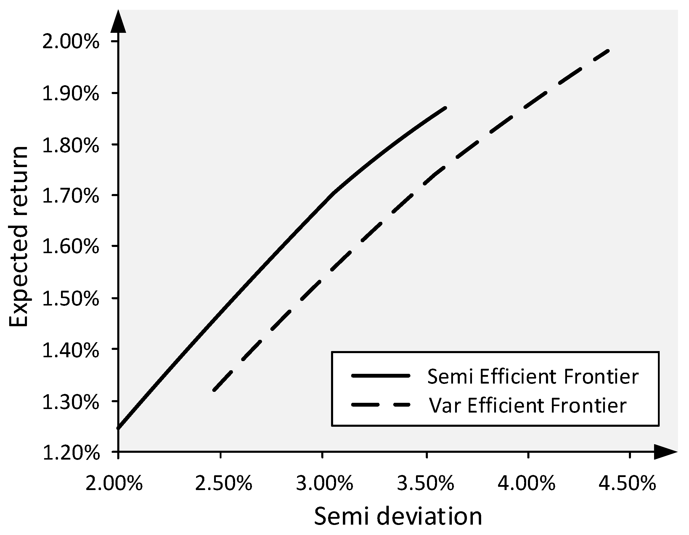
3.4.1. Mean Semi-Variance Model

After the Markowitz mean-variance model, many researchers have attempted to develop and rectify this pattern, including Markowitz himself, who remarked that semi-variance-based analyses create superior stock portfolios than conventional mean-variance-based analysis [52]. Ongoing research on descending risk criteria have sought to replace variance with more appropriate risk criteria.

The semi-variance model works on the same fundamental principle as the variance model, assuming that investors want to reduce the downside risk of investment as much as possible whiteout allowing the rate of return to drop below a certain threshold. The following formula is the definition of semi-variance in the sense of deviations of values below the mean:

$$SV=\sum _{t=1}^T\left[{\left(\sum _{j=1}^n{\tilde{r}}_{jt}{w}_j-\sum _{j=1}^n{r}_j{w}_j\right)}^{2}p\left(t\right)\right]$$

(4)

where SV represents semi-variance, ${\tilde{r}}_{jt}$ denotes the return of asset j from observation t, $w_j$ indicates the weight of the asset j in portfolio, $r_j$ shows the average value (mean) or the expected value of asset j, and $P\left(t\right)$ denotes the probability of event t. For each observation ${\tilde{r}}_j$, it is assumed that

$$\sum _{j=1}^n{\tilde{r}}_{jt}{w}_j\le \sum _{j=1}^n{r}_j{w}_j$$

(5)

Similarly, semi-variance in the sense of deviations of values above the mean can be expressed as

$$SV(>)=\sum _{t=1}^T\left[{\left(\sum _{j=1}^n{\tilde{r}}_{jt}{w}_j-\sum _{j=1}^n{r}_j{w}_j\right)}^{2}p\left(t\right)\right]$$

(6)

with

$$\sum _{j=1}^n{\tilde{r}}_{jt}{w}_j>\sum _{j=1}^n{r}_j{w}_j$$

(7)

Assuming that all observations have the same probability, it follows that $p\left(t\right)=1/T$. To obtain simpler formulation for the semi-variance model, we must consider the following assumption based on the Sharpe beta regression equation:

$${\tilde{r}}_j={\alpha }_j+{\beta }_j·{\tilde{r}}_M+{\tilde{\epsilon }}_j$$

(8)

According to this assumption, there is a relationship between the random variable of return of asset j and the return of the market portfolio ${\tilde{r}}_M$. In this formulation, ${\alpha }_j$ and ${\beta }_j$ are constant values and ${\widetilde{ϵ}}_j$ is a random error with zero covariance for (${\tilde{\epsilon }}_j$,${\tilde{\epsilon }}_h$) and zero covariance for (${\tilde{\epsilon }}_j$, ${\tilde{r}}_M$). Furthermore, ${\beta }_j$ can be calculated using the following equation:

$${\beta }_j=\frac{cov\left({\tilde{r}}_j,{\tilde{r}}_M\right)}{{\sigma }_M^2}$$

(9)

where $cov({\tilde{r}}_j,{\tilde{r}}_M)$ denotes the covariance between the return of asset j and the return of the market portfolio, and ${\sigma }_M^2$ is the variance of the market return. Next, according to Equation  (7), ${\tilde{r}}_j-r_j$ can be calculated as follows:

$${\tilde{r}}_j-r_j={\theta }_j+{\beta }_j·\left({\tilde{r}}_M-r_M\right)$$

(10)

where $r_j$ and $r_M$ are the expected returns of asset j and the market portfolio, respectively, and ${\theta }_j$ has a mean value of zero. The sum of assets for all the assets in the portfolio can be determined from Equation (10):

$$\sum _{j=1}^n\left({\tilde{r}}_j-r_j\right)w_j=\tilde{\theta }+\left({\tilde{r}}_M-r_M\right)\sum _{j=1}^n{\beta }_j{w}_j$$

(11)

where

$$\tilde{\theta }=\sum _{j=1}^n{\tilde{\theta }}_j·w_j$$

(12)

Based on Equation (10), $SV(>)$ can be rewritten as follows:

$$SV(>)=\sum _{\mathrm{t}=1}^{\mathrm{T}}\left[\left(\tilde{\theta }+\left({\tilde{r}}_{\mathrm{M}}-{\mathrm{r}}_{\mathrm{M}}\right)\sum _{\mathrm{j}=1}^{\mathrm{n}}{\beta }_{\mathrm{j}}{w}_{\mathrm{j}}\right){}^{2}p\left(t\right)\right]$$

(13)

When the diversity level reaches infinity, it can be deduced that

$$\underset{L\to \infty }{lim}SV(>)=\left(\sum _{j,h}{\beta }_j{\beta }_h{w}_j{w}_h\right)·SV\left({\tilde{r}}_M>r_M\right)$$

(14)

From to the definition of $SV(<)$ and $SV(>)$, it follows that

$$SV(<)+SV(>)=V=\sum _{t=1}^t{\left[\sum _{j=1}^n{r}_{jt}{w}_j-\sum _{j=1}^n{r}_j{w}_j\right]}^{2}p\left(t\right)$$

(15)

Hence, $SV(<)$ can be obtained by subtracting $SV(>)$ from V as follows:

$$\underset{L\to \infty }{lim}SV(<)=V-\underset{L\to \infty }{lim}SV(>)$$

(16)

$$\underset{L\to \infty }{lim}SV(<)=\sum _{j,h}\left[V_{jh}-{\beta }_j{\beta }_h·SV\left({\tilde{r}}_M>r_M\right)\right]w_j{w}_h$$

(17)

Equation (16) allows the whole process to be implemented with no certain complexity. The semi-variance criterion has been increasingly utilized in studies on descending risk criteria. Grootveld and Hallerbach [53] examined the similarities and dissimilarities between the use of variance or a declining risk criterion, both theoretically and empirically. According to their research, only a small number of the large family of descending risk criteria have superior theoretical characteristics in the risk–return framework than the variance criterion. They investigated the differences between a selection of US asset allocation portfolios on the basis of risk assessment using variance and descending risk metrics. They also discovered that using the downside risk rather than the average variance in the selection process led to slightly higher bond allocation. They also investigated how sampling error can affect expected returns and how risk criteria can affect portfolio composition by performing a simulation, which showed considerable discrepancies in the estimation accuracy, highlighting the need for additional research. Fama [54] and Mandelbrot [55] identified the non-Gaussian nature and skewness of the return distribution. According to the findings of their studies, the return distribution is more extended and skewed than the normal distribution. Quirk and Saposnik [56] demonstrated the significance and superiority of the semi-variance criterion over the conventional variance criterion. Mao [57] demonstrated that investors are more concerned with the unfavorable level of risk as a function of the probability distribution of rate of return than with other deviations. This indicates the behavioral aspect of investor risk aversion, and demonstrates that only the semi-variance criterion should be employed to measure adverse risk.

Arrow [58] stated that by reducing the level of risk aversion among the investors, high-risk assets have become ordinary low-risk assets, which in turn raises the demand for risky assets and ultimately the wealth of investors.

Bawa [59] then developed semi-variance as a risk measurement criterion to reduce the limits on the downward function of risk-averse investors.

Estrada [61] discussed the theoretical frameworks of downside risk. He argued that the mean semi-variance framework is particularly suited for emerging markets [62]. Boasson et al. [63] used a semi-variance technique to estimate the downside risk in optimal portfolio selection. They employed an example of seven exchange-traded index funds (ETFs) representing various types of securities, including government bonds, municipal bonds, investment grade bonds, high-yield bonds, real estate bonds, mortgage-backed securities (MBS), and large capitalization stocks, in order to determine how this method of portfolio optimization by asset allocation based on the mean semi-variance fares against the conventional method. The findings revealed that the mean semi-variance approach offers a number of advantages over the conventional mean-variance approach. Most importantly, it was found that optimization with the semi-variance model produces diverse portfolios that can at least match and at best improve the expected return of portfolios built with the conventional mean-variance model with minimum downside risk.

Boasson et al. [64] obtained the diagram shown in Figure 2, indicating two efficient frontiers where the semi-variance efficient frontier moves to the left-hand side of the variance efficient frontier. They reported that the efficient frontier based on the mean semi-variance framework has a higher risk-return trade-off than that based on the mean-variance framework. They also stated that the final difference between the two efficient frontiers might be much more pronounced if the optimization is performed with a greater number of assets rather than a limited number (seven) of exchange-traded index funds (ETF).

Pla-Santamaria and Bravo [64] used Dow Jones daily stock data from 2005 to 2009 to demonstrate that the mean semi-variance is empirically superior to conventional mean-variance optimization for reflecting downside risks. Liu et al. [65] developed a multi-period portfolio selection model operating based on mean semi-variance optimization in the fuzzy environment.

3.4.2. Mean Absolute Deviation Model

In 1991, the absolute deviation criterion was developed for risk assessment. This criterion measures the deviation from the expected rate of return and transforms it into a linear programming problem, saving considerable calculation time [67]. Using the mean absolute deviation model has an advantage in that the programming problem will be linear rather than quadratic, which means it can be solved without much difficulty using conventional techniques for large-scale optimization problems. This model is defined as  follows:

$$\min \lambda \left[\sum _{t=1}^T\left|r_t-\overline{r}\right|/T\right]-(1-\lambda )\overline{r}$$

(18)

In this formulation, $\overline{r}$ is the average return of the portfolio in the time period $1,2,\cdots ,T$. Using the mean absolute deviation model instead of the mean variance also provides some computational advantages, which have been well proven by Konno [68] and Konno and Koshizuka [69].

Tan Jen Chang et al. [70] examined three measures of variance, semi-variance, and absolute deviation risk to determine how the genetic algorithm (GA) fares against the mean-variance model in the cardinality bounded efficient frontier.

3.4.3. Value at Risk and Conditional Value at Risk Model

The “value at risk” metric, which was proposed in the mid-1990s, is another criterion for quantifying adverse risk. Venture capital offers maximum potential portfolio loss over a specified period with quantitative expression [72]. By definition, value at risk (VaR) is the maximum amount of value loss that can be expected to take place in a portfolio over a given period of time with a given degree of confidence. VAR can also be described as a measure of the worst-case scenario loss that can be expected with a certain probability over a period of time under typical market conditions [73]. The application of this model in risk management as well as for legislative purposes is a criterion for measuring the amount of capital an organization requires to conduct its activities. Due to the unique characteristics of derivative instruments, including the lack of a linear relationship between returns and risk, this index is the only method for calculating risk in investment portfolios that contain a variety of financial derivatives, and other approaches cannot be utilized for this purpose.

The VaR metric possesses mathematically undesirable features, including a lack of convexity. To overcome these undesirable features, Rockafellar and Uryasev introduced the concept of conditional value at risk (CVaR) [71].

Sarykalin et al. [74] presented the diagram shown in Figure 3 to help understand the concepts of VaR, VaR deviation, CVaR, CVaR deviation, max loss, and max loss deviation.

Linsmeier and Pearson [75] proposed the VaR criterion and investigated its three viable solutions, namely historical simulation, parametric simulation, and Monte Carlo simulation, as well as describing the advantages and disadvantages of each method.

Gordon and Baptista [76] compared the mean-variance method with the mean VaR for identifying the optimal stock portfolio. They employed the normal and t-distributions to parametrically estimate VaR, and their research revealed that a portfolio with a higher variance may have a lower VaR for some risk-averse investors.

In a study by Duc Hong Vo et al. [77], they investigated the risk, return and optimal weights of assets in the industry-level market portfolio based on market indices for 10 industries in four countries of Vietnam, Thailand, Malaysia and Singapore from 2007 to 2016. These researchers measured the risk and employed the Markowitz risk–return framework to determine the optimal portfolio composition (weights of assets). The findings of this study showed that among the 10 examined industries, the health care industry should be given high priority in Vietnam and Singapore on account of offering the lowest risk and the highest return because of its dominant role in these two countries. Customer service was found to be the best option in Thailand and Malaysia. In Malaysia, telecommunications was also found to perform well alongside consumer service. Chan et al. [78] tried to determine the VaR of a group of stocks in the mobile phone industry in order to find out which stocks offer the best VaR. The three mobile phone companies studied in this study were Apple Inc., Google Inc., and Microsoft Corporation. They estimated VaR by the use of two non-parametric methods, viz. the basic historical method and the age-weighted historical method, and four parametric methods, viz. the normal distribution, t-distribution, generalized extreme value distribution (GEV) and variance gamma distribution (VG). This study showed that the risk of the examined stocks varies with the method at the 95% confidence level, but Microsoft has the least risky stock with the lowest VaR. With all the methods, the highest VaR was obtained for AAPL, making it the riskiest stock, and the lowest VaR was obtained for MSFT, making it the most stable stock. The conditional coverage test showed the good performance of the historical method among non-parametric methods, and the normal distribution, GEV and VG among parametric methods.

Najafi et al. [79] examined the stock portfolio selection problem using an interval optimization approach. For this purpose, CVaR was used to estimate the expected loss at a certain level of confidence. To manage the uncertainty in the financial markets with the new risk measure, the interval approach was utilized. The good performance of this method in the intended application was illustrated with a numerical example. The results showed that the proposed method is more efficient than the deterministic method.

3.5. Practical Factors

Although the Markowitz mean-variance problem contains a subtle theory for optimal portfolio selection, disregarding real-world considerations may hinder its efficient development for real applications [96]. In addressing this challenge, some researchers have explored practical factors as well as real-world constraints [80,92]. In the following, a number of these studies are introduced.

3.5.1. Transaction Costs

One of the earliest explanations of the problem of mean variance portfolio in the presence of transaction costs was provided by Pogue [81]. Later on, Davis and Norman [82] elaborated on the problem of portfolio selection by introducing commensurate transaction costs. The problem of portfolio optimization with proportional and fixed transaction costs was then formulated and examined by Dumas and Luciano [83] and Morton and Pliska [84]. Yoshimoto [85] derived an optimal portfolio strategy by assuming a V-shaped function for transaction costs. Liu and Loewenstein [147] investigated a problem of portfolio selection, where transaction costs are considered and investors seek to maximize wealth utility over a limited horizons. Oksendal and Sulem [86] examined the problem of portfolio and consumption optimization in the presence of fixed and proportionate transaction costs with the objective of maximizing the expected cumulative utility of consumption over a certain period of time. In a study by Xue et al. [87], they developed a model for mean variance portfolio selection with concave exchange costs. Lobo et al. [88] examined the problem of single-period portfolio optimization with various forms of constraints on potential portfolios and with transaction costs taken into account.

For numerically solving the problem of online portfolio selection, Dai and Zhong  [89] presented a penalty method that includes proportional transaction costs within the framework of mean variance with quadratic transaction costs. In a study conducted by Wang and Liu [90], they formulated the problem of selecting a multi-period mean variance portfolio while taking into account fixed and proportional transaction costs and then defined an indirect utility function to solve the problem with dynamic programming and Lagrange  coefficient.

Fu et al. [91] investigated a multi-period mean-variance portfolio optimization problem with proportional transaction costs. They examined a two-period problem, one of which was deemed risk-free and the other risky. The results demonstrated that transaction costs significantly affect optimal investment decisions.

3.5.2. Real World Constraints

Lim and Zhou [93] explored the subject of optimizing the continuous-time mean-variance portfolio selection by treating interest, appreciation, and volatility rates as random variables. Using the results of convex optimization theory and considering this as a finite linear stochastic-quadratic LQ problem, they extracted the efficient frontier and the associated optimal portfolio. The results indicated that the efficient frontier of mean variance for this problem is a perfect square, indicating that risk-free investment is still viable, even when interest rates are random. This research demonstrated that random LQ control can serve as a robust framework for addressing certain financial application  problems.

Zhu et al. [94] argued that to plan portfolio policies for multiple periods, it is necessary to consider the possibility of bankruptcy prior to the conclusion of each investment horizon. Bankruptcy risk management is therefore an essential element for the optimal selection of a dynamic portfolio. In their research, they introduced a generalized mean-variance model, whereby an optimal investment policy could be developed to allow investors to earn optimal returns, which entails exchanging the mean variance, while also maintaining a high level of bankruptcy risk management.

Xiong and Zhou [95] investigated the problem of continuous-time portfolio selection under the Markowitz mean-variance framework with multiple stocks and bonds in an imperfect market, where past stocks and bond price fluctuations are available information to investors. From the thorough information presented above, efficient strategies are derived, including the optimal filtering of stock growth operations.

3.6. Prediction-Based Models

Numerous studies have been conducted thus far on the predictability and forecasting methods of the stock market. Additionally, there are various theories regarding stock market forecasting in organized markets. Early in the twentieth century, a group of experts in securities valuation firmly believed that a picture for predicting future stock prices could be provided by studying and analyzing the historical trend of stock price fluctuations. More scientific studies, with an emphasis on accurately identifying stock price behavior, have led to a trend toward stock price valuation models. The notion of random steps was initially proposed as a starting point for determining stock price behavior. Experts have utilized a range of techniques over the past two decades to improve stock price forecasting.

In this section, we will review some of these studies. In a study by Enke and Thawornwong [97], they used multiple artificial neural networks, viz. feed forward neural network and generalized regression neural networks to predict changes in stock prices. The results of the neural network models were compared to those of the conventional regression approach and the purchase and maintenance method, indicating that despite the fact that some of these models are superior, the results and predictions are not particularly  satisfactory.

Azar et al. [98] investigated conventional approaches and artificial intelligence for predicting stock price indices and developing a hybrid model. They predicted the price index by employing a number of statistical methods and designing a coupled neural network and a fuzzy model. The results demonstrated that the performance of the combined approach is superior to that of each individual multi-layer neural network, fuzzy neural network, and ARIMA model.

Freitas et al. [99] developed a forecast-based portfolio optimization model that employs normal forecasting errors as a risk metric. They used a novel autoregressive neural network predictor to forecast future stock returns, with its prediction errors serving as a measure of risk. Their results indicated that normal forecasting errors can be obtained with an abnormal series of stock returns and that the portfolio optimization model based on their forecasting outperforms the Markowitz portfolio selection model and yields higher returns for the same risk.

Centeno et al. [100] predicted stock prices using the ARIMA model. On the basis of historical data, expected stock returns were computed and the rate of return variance was analyzed. This study utilized quarterly stock price data from four major US banks between 1 January 2014 and 1 April 2019. An optimization problem was then formulated based on the Markowitz model. This problem was solved by determining the optimal risk portfolio for a future period and estimating an expected rate of return. A comparative analysis of the complete portfolio structure of a risky asset and a risk-free asset was then performed based on the risk aversion factor.

Chen [101] utilized a combination of the ARIMA and Monte Carlo simulation method to predict stock prices. The ARIMA model was used to forecast the stock prices of five popular technology companies, namely, AAPL, AMZN, TSLA, TWTR and MSFT, for the first trading week of September 2021. The Monte Carlo simulation was then used to determine the asset allocation. This combination was compared to the allocation derived from crude Monte Carlo simulations. The results demonstrated that this model is more profitable and accurate than Monte Carlo simulation alone.

Yu et al. [102] improved the portfolio optimization model by integrating performance forecasts and analyzing the results achieved. To ensure the feasibility of the portfolio rebalancing, transaction and borrowing costs were taken into account. The experimental results obtained by analyzing the daily returns provided by international ETFs over a 14-year period demonstrated that using performance forecasting in the optimization model enhances performance through efficient asset allocation, but does not reduce business costs. The models based on the exchange between returns and volatility, such as mean-variance and omega models, were found to perform better than models whose primary focus is loss control, such as value at risk and conditional value at risk. The results demonstrated that when the market fluctuates less, it is more profitable to estimate stock returns.

Ma et al. [103] combined stock return forecasts with a portfolio optimization model. To do this, they employed machine learning methods, including random forest (RF) and support vector regression (SVR), as well as three deep learning models, namely the LSTM neural network, deep multilayer perceptron (DMLP), and convolution neural network (CNN). They initially used these forecasting models to pre-select stocks prior to the formation of the portfolio. Then, they pioneered two novel approaches by combining the prediction results with the mean variance and omega optimization models. Then, the stock portfolio optimization model with an ARIMA algorithm was employed as a criterion to evaluate the superiority of these models. To this end, the nine-year historical data of component stocks of the CSI 100 Index from 2007 to 2015 were collected to perform the validation. The results demonstrated the superior performance of MV and Omega models compared to other models, i.e., RF + MVF and RF + OF. In addition, RF + MVF was found to outperform RF + OF. Accordingly, these researchers stated that investors better build the MVF by predicting the RF return on daily trading investments. In a study by Zhang et al. [148], where these researchers reviewed the developments in the domain of the Markowitz mean-variance model, including the proposals for dynamic, robust, and fuzzy portfolio optimization with the consideration of practical factors, they concluded that the combination of forecasting approaches with portfolio selection methods is likely to result in better robustness against uncertainty.

3.7. Heuristics Methods

Various solution strategies, such as heuristics methods, have been proposed for cardinality-constrained portfolio optimization. For instance, Leung et al. [104] utilized collaborative neurodynamic optimization for portfolio selection. In their study, the conventional MV framework and its variant mean CVaR were formulated as minimax and biobjective portfolio selection problems. Next, neurodynamic approaches were employed to solve these optimization problems. Additionally, particle swarm optimization (PSO)-based weight tuning was adopted to characterize the efficient frontier for each problem using multiple neural networks working collaboratively. Several studies have also applied machine learning techniques for stock selection and portfolio optimization. For instance, Min et al. [105] developed hybrid robust portfolio models, introducing a trade-off parameter to adjust the portfolio optimism level. For this means, they employed different machine learning algorithms, such as long short-term memory (LSTM) and extreme gradient boosting (XGBoost), to evaluate the potential market movements and provide forecasting information to generate the parameter for modeling. Hai et al. [106] developed a machine-learning-based preselection method using random forests (RFs) and support vector machine (SVM), for selecting high-quality risky assets. Chen et al. [107] established a portfolio optimization model based on machine learning, using extreme gradient boosting for the preselection of stocks with greater potential returns prior to employing the mean-variance model.

Some portfolio stock selection approaches address the risk assessment problem using alternative risk or uncertainty metrics besides variance. For instance, Irene Brito [108] introduced a new model for stock selection, the expected utility, entropy, and variance model (EU-EV), which can be utilized as a preselection model for determining optimal mean-variance portfolios. The EU-EV risk model is reliant on entropy, variance, and expected utility, which are coupled via a trade-off parameter. In this study, the selection criterion was based on minimizing the EU-EV risk by reducing the uncertainty caused by variance and entropy and maximizing the expected utility. The proposed methodology involved ranking the stocks of a given set according to their EU-EV risk and selecting the best-ranked stocks with the lowest EU-EV risk in order to produce subsets with fewer stocks than the initial full set of stocks. The mean-variance model was then applied to the subsets including the preselected stocks to generate efficient portfolios. The author drew the conclusion that, with the EU-EV risk model, it is possible to identify the optimal stocks that play the most significant role in the efficient mean–variance portfolio construction. The EU-EV risk model can therefore be utilized as a stock preselection model for the formation of efficient portfolios with a reduced number of stocks.

4. Monte Carlo Simulation

4.1. Monte Carlo Simulation Definition

The Monte Carlo simulation is an approximation technique that employs repeated simulations of system behavior with input variables described by specified probability distribution functions [149].

Metropolis and Ulam [150] published the first paper describing the Monte Carlo method. It is commonly believed that Metropolis selected this name as a reference to the city of Monte Carlo, home of a large casino, and thus as a clear reference to the concept of randomness, which is central to the Monte Carlo method. Over time, there have been numerous developments in the field of statistical simulation in general and the Monte Carlo algorithm in particular. The majority of those advancements have been in the field of natural sciences, particularly physics. However, at the end of the last century, the first academic papers related to the application of the Monte Carlo technique in economics were published. As a result of the continuous evolution and development of modern calculators and programs, Monte Carlo techniques are constantly being improved.

The primary purpose of the Monte Carlo method is to address problems for which there is no clear analytical solution. In all these cases, it should be possible to find an approximation of the solution by repeatedly generating random numbers. The Monte Carlo simulation method is currently utilized in a variety of fields, with financial management and risk management playing a significant role.

4.2. Monte Carlo Simulation in Portfolio Management

Alrabadi and Aljarayesh [109] investigated the capacity of the Monte Carlo simulations to predict the returns of stocks in the Amman Stock Exchange (ASE). They compared the prediction capabilities of the Monte Carlo simulations against those of conventional and exponential moving average techniques during the period from 2003 to 2012. The prediction accuracy was quantified by four different measures: root mean square error (RMSE), mean absolute error (MAE), mean absolute percentage error (MAPE), and Theil’s inequality coefficient (U). The results indicated that the Monte Carlo simulation was the most accurate forecasting technique among those examined.

Tan [110] examined the impact of the COVID-19 pandemic on the financial markets and portfolio management. Using the data of six technology stocks from the American stock market as an example, he constructed the optimal portfolio and the efficient frontier using the Markowitz model and more than 1000 Monte Carlo simulations to perform the portfolio analysis and find the optimal state of the portfolio before and after the epidemic, demonstrated how the outbreak of the pandemic affected investments, and provided recommendations for future portfolio management and construction.

Wu [111] selected 30 stocks from the Chinese A-share market as samples for portfolio analysis based on Markowitz portfolio theory. His goal in this research was to evaluate the validity of Markowitz mean-variance theory and efficient frontier experimentally. He employed Traynor, Sharpe, Jensen, and M2 indicators to evaluate portfolio performance empirically.

Meanwhile, he formed a sample of 1,000,000 portfolio realizations based on the Monte Carlo simulation and empirically demonstrated that both the mean-variance and the efficient frontier theories are valid. However, the reliability of four investment evaluation indicators for investment performance was weak. The author believed that this was probably because the real stock market does not meet some of the assumptions in Markowitz’s  theory.

Determination of Value at Risk Using Monte Carlo Simulation

In the realm of financial risk management, identifying the risk associated with different assets on the stock market is one of the most essential and relevant topics. One of the well-known approaches for measuring, predicting, and managing existing risk is the computation of VaR, which employs a variety of statistical techniques to calculate and measure this risk. In recent years, the application of Monte Carlo simulation has become one of the most important of these techniques, attracting the attention of a great number of researchers [112,113,114,115]. Ghodrati and Zahiri [116] measured the value at risk of 26 chemical companies of the Tehran Stock Exchange during the period from 2009 to 2011 using the Monte Carlo simulation technique with a confidence level of 95%.

Osei et al. [117] compared the historical simulation approach and the Monte Carlo simulation in order to determine VaR. These approaches were applied to six distinct shares on the Ghana stock market with two different confidence levels of 95% and 99%. They stated that the best method for estimating VaR appeared to be the Monte Carlo method. Flexibility is a key advantage of this method. However, its execution is time consuming and necessitates a sophisticated hardware platform.

Azaliney et al. [118] employed three approaches, namely, normal delta, historical simulation, and Monte Carlo simulation, to calculate VaR for a hypothetical portfolio of stocks. The results of this study demonstrated that the Monte Carlo simulation approach is the most practical and flexible method for measuring the VaR compared to the other two methods.

Pasieczna [119] used the Monte Carlo simulation to estimate value at risk. Additionally, the Monte Carlo simulation was employed to estimate the model parameters by fitting real historical data over different periods with certain probability distributions. Simulations were performed for value at risk at 95% and 99% confidence intervals over six estimated periods from 1 to 250 trading days. The results demonstrated that this method is strongly influenced by the choice of the length of historical periods and the past estimation, but this is a reliable method to quantify VaR.

Chijoo Lee [120] tried to develop methods for enhancing the investment interest rate for stock market financing. A combination of the Markowitz model and the Monte Carlo simulation was proposed in this study, which was then validated against the actual interest rate. The proposed method could effectively stimulate investment by enhancing investor interest in the issuance of shares. Yu [121] selected the top ten holdings of China Lombarda Medical Health Fund as a representative portfolio and estimated its VaR using Monte Carlo simulation to provide investors with measurable fund risk information so they could select a more appropriate investment plan.

4.3. Monte Carlo Simulation in Risk Management

Risks are an integral part of every project and the implementation of projects in different sectors requires risk management. A core process of risk management is to identify and analyze risks [122]. The identification of true risks in a project and detailed analysis of these risks tend to result in significant time and cost savings and quality improvement. Many research works in the field of risk management have employed the Monte Carlo simulation method in order to improve risk identification and analysis methods [123,124]. In the following, we will review some of these studies.

Albogamy and Dawood [125] tried to develop an efficient risk assessment technique for client-related risk factors that play a major role in the success of a construction project in its various phases ranging from the preliminary design to the construction and operation. They employed the Monte Carlo simulation method for probability and random variables to effectively control risk factors related to increasing costs and scheduling delays in construction projects. Therefore, the purpose of their study was to provide a technique for a customer-based risk management model. Their proposed method was to integrate the analytical hierarchy process (AHP) with Monte Carlo simulation based on the developed risk plan and evaluate it using a case study.

Arnold et al. [126] used the Monte Carlo simulation to analyze the risk of investment in decentralized renewable energy technologies (RETs) by the use of life cycle representation. The issue they sought to solve was the investors and institutional lenders’ lack of interest in investing in decentralized RETs because of economic barriers, such as undesirable initial capital costs and transaction costs, and the various risks involved in such projects. They stated that to make these investments more attractive, advanced risk management tools are needed to deal with issues related to transaction costs and financial risks. They also noted that using the proposed financial analysis along with Monte Carlo simulation, it is possible to develop a better conceptual design for such investment projects in order to improve their capital return and risk status, and thus raise more capital for investment in technology projects, facilitating decentralized renewable energy. Kumar et al. [127] used the Monte Carlo simulation to develop a standard method of risk modeling for investigating the financial risks that may arise in highway infrastructure projects and how they relate to parameters such as traffic flow and project cost. The approach taken in this study was to use the net present value (NPV) model in combination with the Monte Carlo simulation to analyze the probability distributions of the variety of inputs that may inject uncertainty into NPV. These researchers stated that this method can be used as a tool to decide whether a project will be sufficiently profitable and thus worth the investment. It can also be used to determine what kinds of uncertainty have the greatest impact on the financial performance of the project and help government agencies and officials to determine what measures should be taken to reduce the impacts of these uncertainties on the projects.

5. Application of the Probabilistic Portfolio Management

As described in the introduction section, a precise evaluation of asset risks and returns is crucial for stock portfolio management, given asset prices as a factor to measure returns. On the other hand, due to the volatile nature of the market and the dynamics of the price variation, stock price forecasting plays an important role in developing an efficient strategy for constructing an optimal stock portfolio with high returns, and the results of the forecast are a prerequisite for creating a stock portfolio with an optimal structure. The combination of decision-making methods based on forecasting and then optimizing the stock portfolio can provide a superior approach to conventional methods (i.e., those that use each of the techniques independently for optimization). Additionally, considering the prevailing uncertainty can make the results more practical. Therefore, one of the objectives of this research is to develop a hybrid model to assist investors in selecting the optimal stock  portfolio.

In this section, it is demonstrated how to combine the three primary approaches, i.e., (1) time series forecasting, (2) portfolio optimization, and (3) time-variant probabilistic analysis, to establish the probabilistic portfolio management method for future data. This novel idea is presented in the form of a case study in three separate blocks to provide a benchmark example for similar projects. For this means, among the largest companies (based on their market value) active in the Shanghai Stock Exchange, six companies are selected, whose names and characteristics are presented in

Table 2. Six companies selected from SSE [151].

No.	Company	Sectors	Market Capacity (RMB 10,000) s	Stock Ticker
1	Agricultural Bank of China	Financials–Industry: Diversified Banks	100,095,147.69	601288
2	Bank of Beijing	Financials–Industry: Diversified Banks	8,689,766.54	601169
3	Bank of Communications	Financials–Industry: Diversified Banks	34,309,379.71	601328
4	China Fortune Land Development Co., Ltd.	Real Estate–Industry: Real Estate Investment and Services	978,430.09	600340
5	China pacific insurance	Financials–Industry: Insurance	19,558,154.18	601601
6	China Petroleum & Chemical Corporation	Energy–Industry: Integrated Oil and Gas	51,939,548.94	600028

.

The first three companies are among the largest Chinese banking institutions that are actively engaged in the fields of consumer banking, corporate banking, investment banking, and wealth management among other sectors. The fourth company is a China-based builder and developer of industrial parks and urban real estate. The fifth company is a China-based insurance corporation. The sixth company is an energy corporation, whose main area of activity is the exploration, production, refining, transportation, and sales of oil and gas products. By considering these six companies, a set of stock portfolios is formed, in which the optimal investment method is the ultimate goal of this research. By extracting the data related to these six companies from the Shanghai Stock Exchange from January 2014 to December 2021, six time histories were obtained. The time histories of the close price of these six companies are depicted in Figure 4a, and their rates of return are presented in Figure 4b.

To start the calculations, three categories of conventional pre-processing techniques were applied to the data:

1.

All the data were assessed to fill in the missing data.

2.

The trend and seasonality of the time series were also calculated in order to correctly use the NAR model for time series prediction.

3.

The rate of return of the predicted time series was calculated so that the portfolio optimization process can be implemented accurately.

Next, a time series prediction is used to access their future data from the existing historical data. The NAR method [27,28,29,30] is used for this purpose as follows:

• Importing data into the NAR model and obtaining outputs:

A series of log returns is calculated based on the data collected on the supposed portfolio. The NAR method converts log returns into sequences of numbers 1, 2, and 3. The numbers 1, 2, and 3 correspond to bear days, stagnant days, and bull days, respectively. These numbers are derived by sorting the data from smallest to largest, followed by calculating the mean and standard deviation. The next step is to divide the entire dataset into three parts based on the mean and standard deviation.

• Correlation matrix:

Based on the assumption that each stock in the portfolio is a variable, a correlation is calculated between them. Figure 5 illustrates the correlation among six stocks. A threshold is then imposed on the correlation matrix in order to construct an adjacency matrix. If a correlation between two variables is negative, it will be considered 0; otherwise, it will be considered 1. In the next step, the sum of the rows in the adjacency matrix is computed and stored in a separate vector.

• Data transformation: Assuming N as the number of companies, the ratio of logs of the closed data, $r_{it}$, is defined as follows:

$$r_{it}=\delta log\left(\frac{r_{it}}{r_{it-1}}\right),$$

(19)

where $\delta$ is a constant, which is a hyper parameter in the model. The optimal value of $\delta$ is computed as 0.5.

• NAR model formulation:

Assuming that there are N companies with $r_i={(r_{i1},\cdots ,r_{iT})}^T$ representing the vector of log-returns of their stock prices, the proposed network auto-regression (NAR) model is formulated as

$$r_{it}={\beta }_0+{\beta }_1{n}_i^{-1}\sum _{j=1}^N{a}_{ij}{r}_{j(t-1)}+{\beta }_2{r}_{i(t-1)}+{\epsilon }_{it},$$

(20)

where $r_{it}$ is the log return of company i at time t. The cross-correlations among companies i and j are calculated as follows:

$$c_{ij}\equiv \frac{〈r_i{r}_j〉-〈r_i〉〈r_j〉}{\sqrt{\left(〈r_i^2〉-{〈r_i〉}^2\right)\left(〈r_j^2〉-{〈r_j〉}^2\right)}},$$

(21)

Here, the brackets indicate the average temporal value over the companies during the desired period. The correlation between companies i and j, $c_{ij}$, can vary between $[-1,1]$. A $c_{ij}$ value of $1(-1)$ indicates complete correlation (i.e., anti-correlation) between two companies, whereas a $c_{ij}$ value of 0 implies that they are uncorrelated.

The adjacency matrix of correlation between the log-returns of N companies with zero diagonal is denoted by $A={\left(a_{ij}\right)}_{N\times N}$ and constructed as follows:

• where $\theta$ is a hyper-parameter which should be determined by try and error. In cases where $i\ne j$, the total sum of adjacency matrix is calculated as $n_i={\sum }_{j=1}^N{a}_{ij}$. Additionally, $E\left({\epsilon }_{it}\right)=0$, $Var\left({\epsilon }_{it}\right)={\sigma }^2$, and ${\epsilon }_{it}$ follows the normal distribution. A matrix representation of Equation (20) can be provided as follows:

$$\begin{gathered} \begin{array}{c}{\left(r_{1t},...,r_{Nt}\right)}^{⊺}={(1,...,1)}^{⊺}{\beta }_0+{\beta }_1\left(\begin{array}{ccccc}\frac{1}{n_1}& 0& \cdots & 0& \\ 0& \frac{1}{n_2}& \cdots & 0\\ ⋮& & \ddots & 0\\ 0& \cdots & 0& \frac{1}{n_N}\end{array}\right)A+{\beta }_2\left(\begin{array}{ccccc}1& 0& \cdots & 0& \\ 0& 1& \cdots & 0\\ ⋮& & \ddots & 0\\ 0& \cdots & 0& 1\end{array}\right)\end{array} \\ +(r_{1(t-1)},...,r_{N(t-1)})+{({\epsilon }_{1t},...,{\epsilon }_{Nt})}^{⊺} \end{gathered}$$

(22)

or concisely, it can be rewritten as:

$$R_t=A_0+G{R}_{t-1}+{\epsilon }_{Rt}$$

(23)

where $R_t=(r_{1t},...,r_{Nt})\in R^N$, $A_0={\beta }_1\mathbf{1}$ where in $\mathbf{1}=(1,...,1)$, $G={\beta }_{1}W+{\beta }_2\mathbf{I}$ in which $W=diag\{n_1^{-1},...,n_N^{-1}\}A$, and $\mathbf{I}$ is an identity matrix.

In the NAR model framework, three characteristics are observed: (1) $r_{it}$ might be affected by itself but from the previous time point, $r_{i(t-1)}$, referred to as the autoregressive effect; (2) $r_{it}$ might be affected by other companies, which are collected by $\{j:a_{ij}=1\}$, known as the market effect; and (3) the unexplained variation is attributed to an independent random noise,${\epsilon }_{it}$. For example, for a company $i=1$ at $t=2$, $r_{12}$ is calculated as follows:

$$\begin{array}{cc}\hfill r_{12}& ={\beta }_0+\underset{\mathrm{Market}\mathrm{effect}}{\underbrace{{\beta }_1{n}_1^{-1}\sum _{j=1}^N{a}_{1j}{r}_{j2}}}+\stackrel{\mathrm{authoregresive}\mathrm{effect}}{\overbrace{{\beta }_2{r}_{12}}}+\underset{\mathrm{independent}\mathrm{noise}}{\underbrace{{\epsilon }_{12}}}\hfill \\ \hfill & ={\beta }_0+{\beta }_1\frac{a_{12}{r}_{22}+\cdots +a_{1N}{r}_{N2}}{a_{12}+\cdots +a_{1N}}+{\beta }_2{r}_{12}+{\epsilon }_{12}.\hfill \end{array}$$

(24)

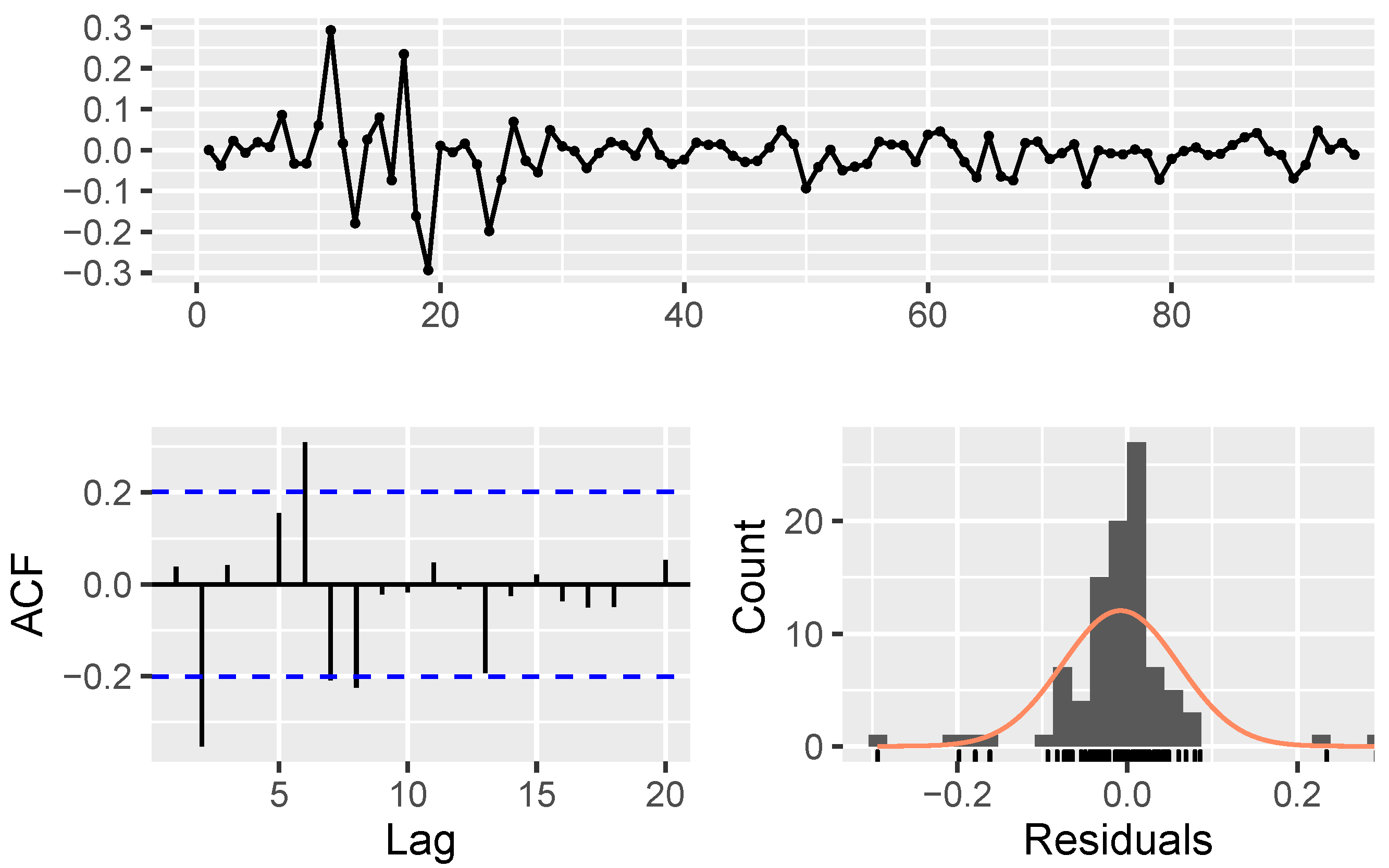
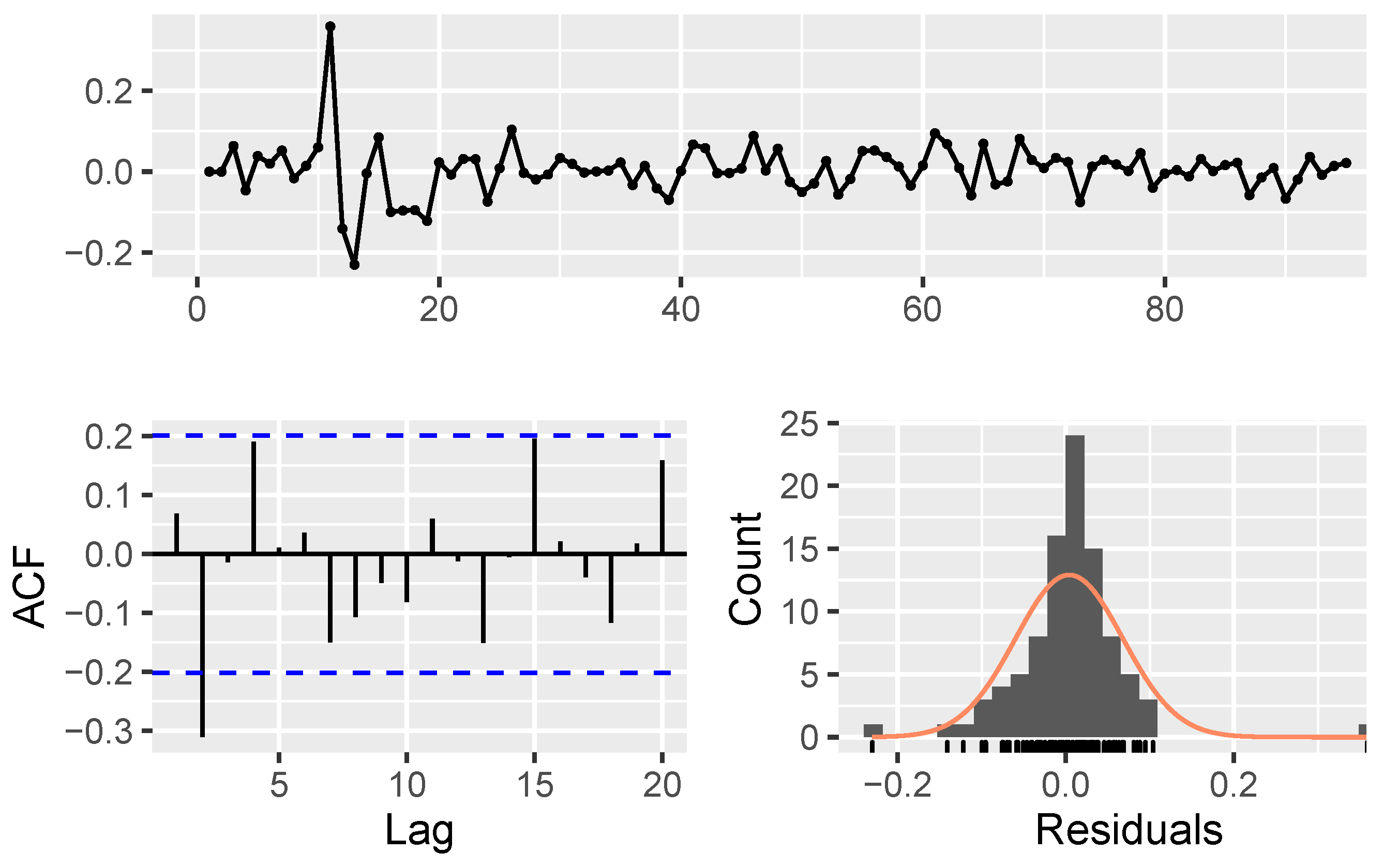
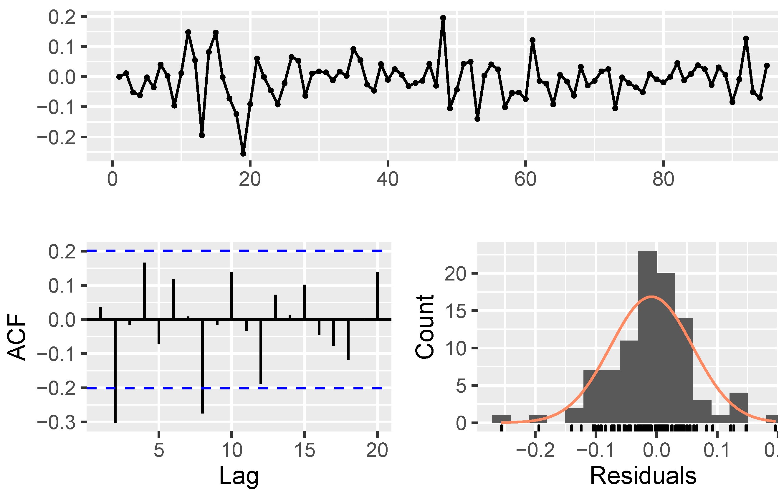
• Model parameters estimation and validation:

The maximum likelihood estimation (MLE) is adopted as follows to provide an estimation of $\theta =({\beta }_0,{\beta }_1,{\beta }_2)$:

$$mi{n}_{\theta }\left|R_t-A_0-G{R}_{t-1}\right|.$$

(25)

Afterwards, Equation (20) can be rewritten as follows:

$$r_{it}=X_{i(t-1)}^{\top }\theta +{\epsilon }_{it},$$

(26)

where $X_{i(t-1)}={\left(1,w_i^{\top }{r}_{t-1},r_{i(t-1)}\right)}^{\top }$ and $w_i=\left(\frac{a_{ij}}{n_i}:1\le j\le N\right)$ is the ith row of W. Next, the maximum likelihood estimator of $\theta$ reads as follows:

$$\widehat{\theta }=\theta +{\left(\sum _{t=1}^T{X}_{t-1}^{\top }{X}_{t-1}\right)}^{-1}\sum _{t=1}^T{X}_{t-1}^{\top }{\epsilon }_{Rt}.$$

(27)

The model performance can be assessed utilizing the root mean square error (RMSE) as follows:

$$RMSE\left(i\right)=\sqrt{\frac{1}{T}\sum _{t=1}^T{(r_{it}-{\widehat{r}}_{it})}^2},$$

(28)

where ${\widehat{r}}_{it}$ is the log-returns derived from the NAR model.

The whole process of NAR model is summarized in in Algorithm 1 shown as follows:

Algorithm 1: The procedure of modeling using NAR

Data: fetching stock price data Result: estimating $\beta =({\beta }_0,{\beta }_1,{\beta }_2)$. The initialization; Transforming data by Equation 19; Creating correlation matrix, $c_{ij}$;

Figure 6 illustrates the transformed data for Stock 1 as well as the log-return data obtained from the NAR and ARIMA models. On the basis of the RMSE measure, the results for both models are presented in

Table 3. RMSE metric of ARIMA and NAR models for 6 companies.

No	Company	ARIMA Model’s RMSE	ARIMA Model Parameters (p,d,q)	NAR Model’s RMSE
1	Agricultural Bank of China	9.23	(1,1,1)	3.45
2	Bank of Beijing	9.32	(1,1,1)	3.54
3	Bank of Communications	9.11	(1,2,1)	3.32
4	China Fortune Land Development Co., Ltd.	9.03	(1,1,1)	3.23
5	China pacific insurance	9.54	(1,2,2)	3.67
6	China Petroleum & Chemical Corporation	9.16	(1,1,1)	3.38

, in which the NAR model outperforms the ARIMA model in all companies. The residual plots of ARIMA model for all six companies are provided in Appendix A. Figure 7 depicts the point forecasts as well as 80% and 95% forecast intervals for the upcoming two years for all six stocks.

The deterministic time-series forecasting methods that are conventionally used to forecast the future generally do not provide accurate and reliable forecasts of fluctuations. However, the combination of this method with Monte Carlo sampling made prevailing uncertainty in price fluctuations to be included in the output of the model. This enabled the model to provide an exceedance probability of the stock price instead of deterministic prediction of stock price in the future. This result demonstrates the superiority of the proposed method over conventional deterministic approaches. For this purpose, one thousand random samples are generated for the existing time series using the Monte Carlo sampling method. Next, each batch of the resulting random samples is imported into the NAR model to predict their corresponding time series for the next two years. Hence, one thousand predictions of the future of the target stock are obtained. These outputs are depicted in Figure 8.

By having time series calculated for the future timeframe, a thousand of stock price samples are calculated at each point in time. This result makes it feasible to determine an exceedance probability at any point in time and for any stock price level. By carrying out this procedure across the entire time period and plotting the corresponding probability contour, Figure 9 is obtained. As seen in this figure, the stock price can be predicted for each distinct level of exceedance probability and desired time. In other words, it is possible to estimate in terms of probability what the stock price will be at any given time.

Figure 9 depicts the exceedance probability of the stock close price over time. The advantage of this presentation of time-series prediction compared to conventional methods is that it can model the uncertainty in the data. That is, the model’s output is not limited to a specific value of the stock price at the desired time but its probability distribution in time. In other words, the prediction method provides the output considering different random scenarios in terms of probability contours. In this way, it is possible to predict the expected price by selecting a target probability level (acceptable risk level) at the desired time. By repeating this for all other companies, a comparison can be made between them to make an optimized investment decision.

In the following, each of the random realizations resulting from the Monte Carlo sampling method is utilized as an input for portfolio optimization.

In this research, the optimal portfolio was obtained using mean semi-variance optimization model. This model works on the same basic principle as the mean-variance model, with the difference that values lower than the mean are considered portfolio risk. The multi-objective mean semi-variance optimization model is defined as follows:

$$\begin{array}{c}max:{\mu }_p=w^T\mu ={\displaystyle \sum _{i=1}^n}{w}_i{\mu }_i\\ min:{\sigma }_{p^{-}}^2=w^T{\displaystyle \sum _{-}}w={\displaystyle \sum _{i=1}^n}{\displaystyle \sum _{j=1}^n}{w}_i{w}_j{\sigma }_{i{j}^{-}}\\ \mathrm{subject}\mathrm{to}:{\displaystyle \sum _i}{w}_i=1\\ w_i\ge 0i=1\dots n\end{array}$$

(29)

where ${\mu }_p$ represents the expectation of the portfolio return, ${\mu }_i$ denotes the expectation of the asset i, $w_i$ and $w_j$ represent the fraction of the total portfolio value that is invested in asset i and j, respectively, and ${\sigma }_{(ij-)}$ represents the portfolio risk lower than the mean.

In this way, instead of a deterministic efficient frontier, a thousand efficient frontiers are obtained. In other words, the efficient frontier itself depends on a level of probability. The set of efficient frontiers corresponding to 1000 generated random samples is illustrated in Figure 10a, and the probabilistic form of the efficient frontier is presented in Figure 10b.

Moreover, each of the random realizations corresponds to an optimal distribution of assets. In other words, a thousand optimal capital distributions are obtained. These data can then be used to generate optimal capital probability distributions. The results are depicted in the form of a histogram of investment weight per stock in Figure 11.

It has significant advantages over deterministic methods for expressing the capital distribution of companies, including the following:

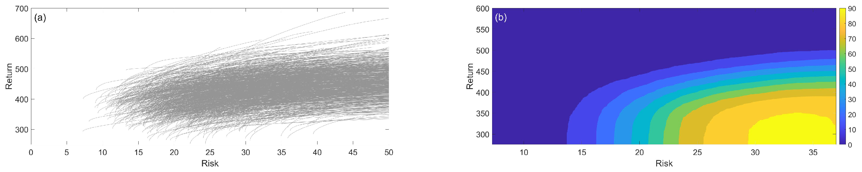
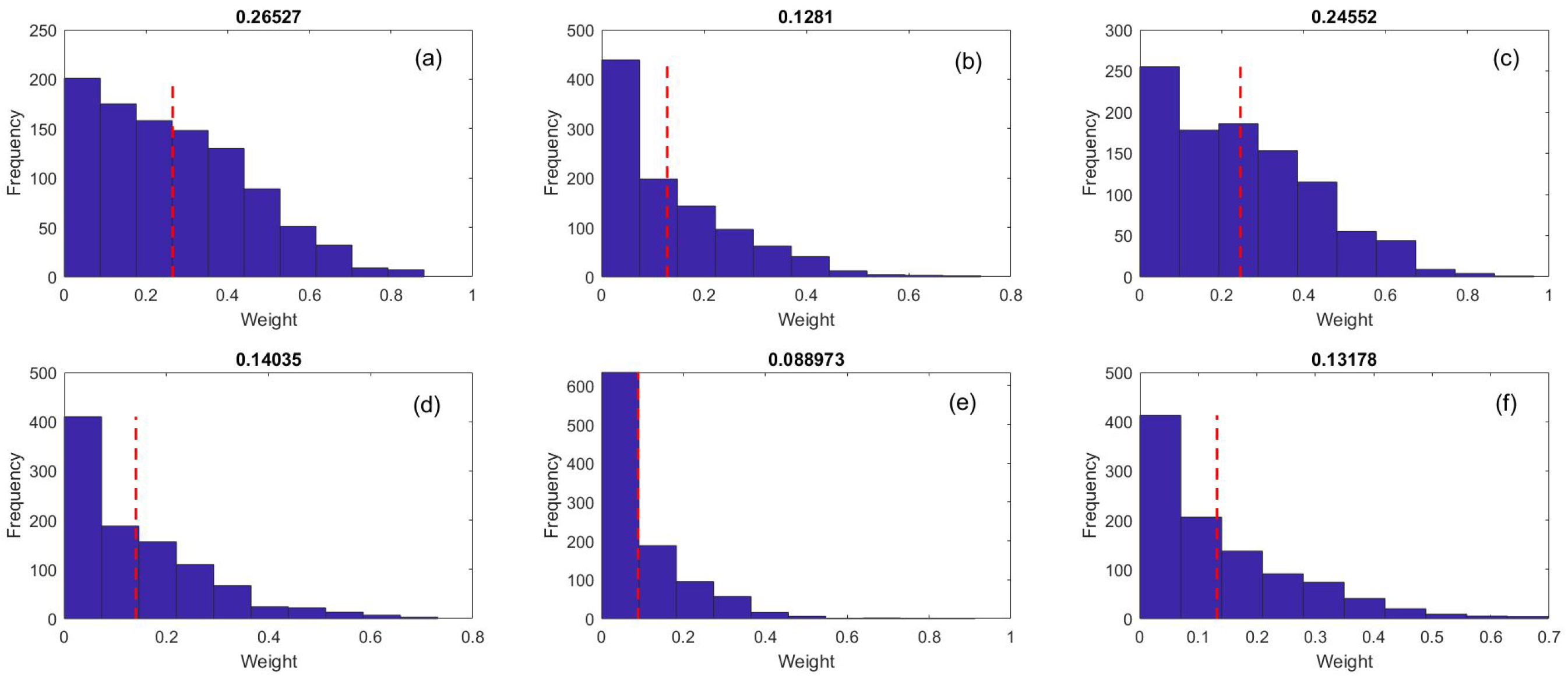
• Given the entire histogram, investors can obtain a more comprehensive view of investment risk, which allows them to set the size of their investment in each company.
• In this investment estimation, uncertainty is taken into account, thereby preventing the output from being confined to one deterministic sample.
• The histogram of investment weight shows what proportion of the generated random realizations corresponds to what amount of investment.
• This expression of investment goes beyond a deterministic expression. That is, in addition to stating the determination of the amount of investment, it also provides its probability distribution.

6. Conclusions

In this paper, the probabilistic portfolio optimization methods using future data were reviewed. For this purpose, various time-series analysis methods for stock market data were categorized and described. A variety of portfolio optimization methods were investigated and various studies in this field were examined and compared. Furthermore, the Monte Carlo sampling method was discussed following a discussion on how to implement it for stock market analysis. Various studies that employed the Monte Carlo sampling method to implement portfolio management were also categorized and reviewed.

The data pertaining to the Shanghai Stock Exchange were analyzed as a case study. The NAR time series prediction algorithm was then proposed to forecast future stock market data. This algorithm was then combined with the Monte Carlo sampling method to provide a probabilistic form of time series prediction. The paper also explained how the mean semi-variance optimization method is incorporated into the problem, and finally presented the probabilistic form of portfolio management for future data. The most important results of this review paper are summarized below:

• Using future stock market data instead of historical data provides a more appropriate estimate of stock portfolio risk and return.
• By approximating the time series in the form of a random process by the Monte Carlo sampling method, it can well capture the prevailing uncertainty.
• The portfolio optimization method can be well combined with the random realizations resulting from the Monte Carlo sampling method to provide a probabilistic form of portfolio management.

The findings of this study can be utilized by individual and institutional investors, such as companies and investment funds. However, this study also faces a number of limitations. For the sake of brevity, the most influential studies were reviewed in the literature review section. There are more studies undertaken in these areas, which can be found in the literature. Additionally, in the case study section, historical data were used as input features in the stock forecasting process. In a more general structure, the performance of the forecasting model can be measured using macroeconomic criteria, such as technical, financial, and economic indicators. Furthermore, the case study was implemented with three selected methods for each of the triple modules of time series forecasting, portfolio optimization, and probabilistic analysis. These modules can be potentially implemented with any chosen method, which can be investigated in other projects. Overall, future studies can enhance the performance of the method by incorporating additional input features and more complex risk criteria in the construction of forecast-based portfolio models. In addition, other types of models, such as artificial neural networks and Bayesian statistical methods, can assist in optimizing the investment portfolio, bringing the expected return closer to the actual return, and achieving the objective of maximizing profitability. These issues will be under investigation by the authors in future studies.

References

1. Billah, B.; King, M.L.; Snyder, R.D.; Koehler, A.B. Exponential smoothing model selection for forecasting. Int. J. Forecast. 2006, 22, 239–247. [Google Scholar] [CrossRef] [Green Version]
2. de Faria, E.; Albuquerque, M.P.; Gonzalez, J.; Cavalcante, J.; Albuquerque, M.P. Predicting the Brazilian stock market through neural networks and adaptive exponential smoothing methods. Expert Syst. Appl. 2009, 36, 12506–12509. [Google Scholar] [CrossRef]
3. Dutta, A.; Bandopadhyay, G.; Sengupta, S. Prediction of Stock Performance in the Indian Stock Market Using Logistic Regression. Int. J. Bus. Information 2012, 7, 105–136. [Google Scholar]
4. Devi, B.U.; Sundar, D.; Alli, P. An Effective Time Series Analysis for Stock Trend Prediction Using ARIMA Model for Nifty Midcap-50. Int. J. Data Min. Knowl. Manag. Process. 2013, 3, 65–78. [Google Scholar] [CrossRef]
5. Wang, J.J.; Wang, J.Z.; Zhang, Z.G.; Guo, S.P. Stock index forecasting based on a hybrid model. Omega 2012, 40, 758–766. [Google Scholar] [CrossRef]
6. Rahman, A.; Hasan, M.M. Modeling and Forecasting of Carbon Dioxide Emissions in Bangladesh Using Autoregressive Integrated Moving Average (ARIMA) Models. Open J. Stat. 2017, 7, 560–566. [Google Scholar] [CrossRef] [Green Version]
7. Usha, T.M.; Balamurugan, S.A.A. Seasonal Based Electricity Demand Forecasting Using Time Series Analysis. Circuits Syst. 2016, 7, 3320–3328. [Google Scholar] [CrossRef] [Green Version]
8. Nerlove, M.; Diebold, F.X. Time Series Analysis. In Time Series and Statistics; Palgrave Macmillan UK: London, UK, 1990; pp. 294–309. [Google Scholar] [CrossRef]
9. Ho, S.; Xie, M. The use of ARIMA models for reliability forecasting and analysis. Comput. Ind. Eng. 1998, 35, 213–216. [Google Scholar] [CrossRef]
10. Shumway, R.H.; Stoffer, D.S. Time Series: A Data Analysis Approach Using R; Chapman and Hall/CRC: Boca Raton, FL, USA, 2019. [Google Scholar] [CrossRef]
11. Ariyo, A.A.; Adewumi, A.O.; Ayo, C.K. Stock Price Prediction Using the ARIMA Model. In Proceedings of the 2014 UKSim-AMSS 16th International Conference on Computer Modelling and Simulation, Cambridge, UK, 26–28 March 2014; pp. 106–112. [Google Scholar] [CrossRef] [Green Version]
12. Bhuriya, D.; Kaushal, G.; Sharma, A.; Singh, U. Stock market predication using a linear regression. In Proceedings of the 2017 International conference of Electronics, Communication and Aerospace Technology (ICECA), Coimbatore, India, 20–22 April 2017; pp. 510–513. [Google Scholar] [CrossRef]
13. Liu, W.; Morley, B. Volatility Forecasting in the Hang Seng Index using the GARCH Approach. Asia-Pac. Financ. Mark. 2009, 16, 51–63. [Google Scholar] [CrossRef]
14. Engle, R.F. Autoregressive Conditional Heteroscedasticity with Estimates of the Variance of United Kingdom Inflation. Econometrica 1982, 50, 987. [Google Scholar] [CrossRef]
15. Mahajan, V.; Thakan, S.; Malik, A. Modeling and Forecasting the Volatility of NIFTY 50 Using GARCH and RNN Models. Economies 2022, 10, 102. [Google Scholar] [CrossRef]
16. Haas, M.; Pigorsch, C. Financial Economics, Fat-Tailed Distributions. In Complex Systems in Finance and Econometrics; Springer: New York, NY, USA, 2009; pp. 308–339. [Google Scholar] [CrossRef]
17. Shi, F.; Sun, X.Q.; Gao, J.; Wang, Z.; Shen, H.W.; Cheng, X.Q. The prediction of fluctuation in the order-driven financial market. PLoS ONE 2021, 16, e0259598. [Google Scholar] [CrossRef]
18. Budiharto, W. Data science approach to stock prices forecasting in Indonesia during Covid-19 using Long Short-Term Memory (LSTM). J. Big Data 2021, 8, 47. [Google Scholar] [CrossRef]
19. Cheteni, P. Stock Market Volatility Using GARCH Models: Evidence from South Africa and China Stock Markets. J. Econ. Behav. Stud. 2017, 8, 237–245. [Google Scholar] [CrossRef] [Green Version]
20. Nelson, D.B. ARCH models as diffusion approximations. J. Econom. 1990, 45, 7–38. [Google Scholar] [CrossRef]
21. Wang, Y.; Xiang, Y.; Lei, X.; Zhou, Y. Volatility analysis based on GARCH-type models: Evidence from the Chinese stock market. Econ.-Res.-Ekon. IstražIvanja 2022, 35, 2530–2554. [Google Scholar] [CrossRef]
22. Li, W.K.; Mak, T.K. On the Squared Residual Autocorrelations in Non-linear Time Series with Conditional Heteroskedasticity. J. Time Ser. Anal. 1994, 15, 627–636. [Google Scholar] [CrossRef]
23. Ma, J.; Liu, L. Multivariate Nonlinear Analysis and Prediction of Shanghai Stock Market. Discret. Dyn. Nat. Soc. 2008, 2008, 1–8. [Google Scholar] [CrossRef]
24. Nobi, A.; Maeng, S.E.; Ha, G.G.; Lee, J.W. Effects of global financial crisis on network structure in a local stock market. Phys. Stat. Mech. Its Appl. 2014, 407, 135–143. [Google Scholar] [CrossRef]
25. Zhang, W.; Zhuang, X. The stability of Chinese stock network and its mechanism. Phys. Stat. Mech. Its Appl. 2019, 515, 748–761. [Google Scholar] [CrossRef]
26. Tabak, B.M.; Serra, T.R.; Cajueiro, D.O. Topological properties of stock market networks: The case of Brazil. Phys. Stat. Mech. Its Appl. 2010, 389, 3240–3249. [Google Scholar] [CrossRef]
27. Sioofy, K.A.; Han, D. Network analysis of the Chinese stock market during the turbulence of 2015–2016 using log-returns, volumes and mutual information. Phys. Stat. Mech. Its Appl. 2019, 523, 1091–1109. [Google Scholar] [CrossRef]
28. Sioofy, K.A.; Dong, H. Topological Structure of Stock Market Networks during Financial Turbulence: Non-Linear Approach. Univers. J. Account. Financ. 2019, 7, 106–121. [Google Scholar] [CrossRef]
29. Sioofy, K.A.; Han, D. Stock price network autoregressive model with application to stock market turbulence. Eur. Phys. J. 2020, 93, 133. [Google Scholar] [CrossRef]
30. Sioofy, K.A.; Mahsuli, M.; Shadabfar, M.; Hosseini, V.R.; Kordestani, H. A proposed fractional dynamic system and Monte Carlo-based back analysis for simulating the spreading profile of COVID-19. Eur. Phys. J. Spec. Top. 2022, 231, 3427–3437. [Google Scholar] [CrossRef]
31. Ban, G.Y.; El Karoui, N.; Lim, A.E. Machine Learning and Portfolio Optimization. Manag. Sci. 2018, 64, 1136–1154. [Google Scholar] [CrossRef] [Green Version]
32. Francesco, C.; Andrea, S.; Tardella, F. Linear vs. quadratic portfolio selection models with hard real-world constraints. Comput. Manag. Sci. 2014, 12, 345–370. [Google Scholar]
33. Nasim, D.H.; Abolfazl, K.; Markku, K.; Korhonen, P. Solving cardinality constrained mean-variance portfolio problems via MILP. Ann. Oper. Res. 2017, 254, 47–59. [Google Scholar]
34. Strumberger, I.; Bacanin, N.; Tuba, M. Constrained Portfolio Optimization by Hybridized Bat Algorithm. In Proceedings of the 2016 7th International Conference on Intelligent Systems, Modelling and Simulation, Bangkok, Thailand, 25–27 January 2016; pp. 83–88. [Google Scholar] [CrossRef]
35. Zaheer, H.; Pant, M. Solving Portfolio Optimization Problem through Differential Evolution. In Proceedings of the International Conference on Electrical, Electronics, and Optimization Techniques (ICEEOT), Chennai, India, 3–5 March 2016; pp. 3982–3987. [Google Scholar] [CrossRef]
36. Xia, Y.; Liu, B.; Wang, S.; Lai, K.K. A model for portfolio selection with order of expected returns. Comput. Oper. Res. 2000, 27, 409–422. [Google Scholar] [CrossRef]
37. Liu, Y. An Empirical Portfolio Study Based on Markowitz Theory. In Proceedings of the 7th International Conference on Financial Innovation and Economic Development, Online, 14–16 January 2022; pp. 397–404. [Google Scholar]
38. Hadi, A.S.; El Naggar, A.A.; Abdel Bary, M.N. New model and method for portfolios selection. Appl. Math. Sci. 2016, 10, 263–288. [Google Scholar] [CrossRef]
39. Qu, B.Y.; Zhou, Q.; Xiao, J.M.; Liang, J.J.; Suganthan, P.N. Large-Scale Portfolio Optimization Using Multiobjective Evolutionary Algorithms and Preselection Methods. Math. Probl. Eng. 2017, 2017, 1–14. [Google Scholar] [CrossRef] [Green Version]
40. Bili, C.; Yangbin, L.; Wenhua, Z.; Hang, X.; Zhang, D. The mean-variance cardinality constrained portfolio optimization problem using a local search-based multi-objective evolutionary algorithm. Appl. Intell. 2017, 47, 505–525. [Google Scholar] [CrossRef]
41. Jalota, H.; Thakur, M. Genetic algorithm designed for solving portfolio optimization problems subjected to cardinality constraint. Int. J. Syst. Assur. Eng. Manag. 2017, 9, 294–305. [Google Scholar] [CrossRef]
42. Miryekemami, S.A.; Sadeh, E.; Sabegh, Z.A. Using Genetic Algorithm in Solving Stochastic Programming for Multi-Objective Portfolio Selection in Tehran Stock Exchange. Adv. Math. Financ. Appl. 2017, 2, 107–120. [Google Scholar]
43. Zhao, P.; Gao, S.; Yang, N. Solving Multi-Objective Portfolio Optimization Problem Based on MOEA/D. In Proceedings of the 12th International Conference on Advanced Computational Intelligence (ICACI), Dali, China, 14–16 August 2020; pp. 30–37. [Google Scholar]
44. Samuelson, P.A. Lifetime portfolio selection by dynamic stochastic programming. Rev. Econ. Stat. 1969, 51, 239–246. [Google Scholar] [CrossRef]
45. Grauer, R.R.; Hakansson, N.H. On the use of mean-variance and quadratic approximations in implementing dynamic investment strategies: A comparison of returns and investment policies. Manag. Sci. 1993, 39, 856–871. [Google Scholar] [CrossRef]
46. Merton, R.C. Lifetime portfolio selection under uncertainty: The continuous-time case. Rev. Econ. Stat. 1969, 51, 247–257. [Google Scholar] [CrossRef] [Green Version]
47. Karatzas, I.; Lehoczky, J.P.; Shreve, S.E. Optimal portfolio and consumption decisions for a “small investor” on a finite horizon. Siam J. Control. Optim. 1987, 25, 1557–1586. [Google Scholar] [CrossRef] [Green Version]
48. Bajeux-Besnainou, I.; Portait, R. Dynamic Asset Allocation in a Mean-Variance Framework. Manag. Sci. 1998, 44, 79–95. [Google Scholar] [CrossRef]
49. Li, D.; Ng, W.L. Optimal Dynamic Portfolio Selection: Multiperiod Mean-Variance Formulation. Math. Financ. 2000, 10, 387–406. [Google Scholar] [CrossRef]
50. Yi, L.; Li, Z.F.; Li, D. Multi-period portfolio selection for asset-liability management with uncertain investment horizon. J. Ind. Manag. Optim. 2008, 4, 535–552. [Google Scholar] [CrossRef]
51. Sun, Y.; Aw, G.; Teo, K.L.; Yanjian Zhu, X.W. Multi-period Portfolio Optimization Under Probabilistic Risk Measure. Financ. Res. Lett. 2016, 18, 60–66. [Google Scholar] [CrossRef]
52. Markowitz, H.; Todd, P.; Xu, G.; Yamane, Y. Computation of mean-semivariance efficient sets by the Critical Line Algorithm. Ann. Oper. Res. 1993, 45, 307–317. [Google Scholar] [CrossRef]
53. Henk Grootveld, W.H. Variance vs downside risk: Is there really that much difference? Eur. J. Oper. Res. 1999, 114, 304–319. [Google Scholar] [CrossRef]
54. Fama, E.F. Mandelbrot and the Stable Paretian Hypothesis. J. Bus. 1963, 36, 420–429. [Google Scholar] [CrossRef] [Green Version]
55. Mandelbrot, B. The Variation of Certain Speculative Prices. J. Bus. 1963, 36, 371–418. [Google Scholar] [CrossRef]
56. Quirk, J.P.; Saposnik, R. Admissibility and measurable utility functions. Rev. Econ. Stud. 1962, 29, 140–146. [Google Scholar] [CrossRef]
57. Mao, J.C.T. Models of Capital Budgeting, E-V Vs E-S. J. Financ. Quant. Anal. 1970, 4, 657–675. [Google Scholar] [CrossRef]
58. Arrow, K.J. Essays in the Theory of Risk-Bearing Paperback; North-Holland Pub. Co.: Amsterdam, The Netherlands, 1970. [Google Scholar]
59. Bawa, V.S. Optimal rules for ordering uncertain prospects. J. Financ. Econ. 1975, 2, 95–121. [Google Scholar] [CrossRef]
60. Foo, T.; Eng, S. Asset allocation in a downside risk framework. J. Real Estate Portf. Manag. 2000, 6, 213–223. [Google Scholar] [CrossRef]
61. Estrada, J. Downside Risk in Practice. J. Appl. Corp. Financ. 2006, 18, 117–125. [Google Scholar] [CrossRef]
62. Estrada, J. Mean-Semivariance Behaviour: An Alternative Behavioural Model. J. Emerg. Mark. Financ. 2004, 3. [Google Scholar] [CrossRef]
63. Boasson, V.; Boasson, E.; Zhou, Z. Portfolio optimization in a mean-semivariance framework. Invest. Manag. Financ. Innov. 2011, 8, 58–68. [Google Scholar]
64. Pla-Santamaria, D.; Bravo, M. Portfolio optimization based on downside risk: A mean-semivariance efficient frontier from Dow Jones blue chips. Ann. Oper. Res. 2013, 205, 189–201. [Google Scholar] [CrossRef]
65. Liu, Y.J.; Zhang, W.G. A multi-period fuzzy portfolio optimization model with minimum transaction lots. Eur. J. Oper. Res. 2015, 242, 933–941. [Google Scholar] [CrossRef]
66. Konno, H.; Yamazaki, H. Mean -Absolute Deviation Portfolio Optimization Model and Its Applications to Tokyo Stock Market. Manag. Sci. 1991, 37, 519–531. [Google Scholar] [CrossRef] [Green Version]
67. Chaiyakan, S.; Thipwiwatpotjana, P. Bounds on mean absolute deviation portfolios under interval-valued expected future asset returns. Comput. Manag. Sci. 2021, 18, 195–212. [Google Scholar] [CrossRef]
68. Konno, H. Portfolio optimization of small scale fund using mean-absolute deviation model. Int. J. Theor. Appl. Financ. 2003, 6, 403–418. [Google Scholar] [CrossRef]
69. Konno, H.; Koshizuka, T. Mean-absolute deviation model. Iie Trans. 2005, 37, 893–900. [Google Scholar] [CrossRef]
70. Chang, T.J.; Yang, S.C.; Chang, K.J. Portfolio optimization problems in different risk measures using genetic algorithm. Expert Syst. Appl. 2009, 36, 10529–10537. [Google Scholar] [CrossRef]
71. Rockafellar, R.T.; Uryasev, S. Optimization of conditional value-at-risk. J. Risk 2000, 2, 21–42. [Google Scholar] [CrossRef] [Green Version]
72. Jorion, P. How informative are value-at-risk disclosures? Account. Rev. 2002, 77, 911–931. [Google Scholar] [CrossRef]
73. Abad, P.; Benito, S.; López, C. A comprehensive review of Value at Risk methodologies. Span. Rev. Financ. Econ. 2014, 12, 15–32. [Google Scholar] [CrossRef]
74. Sarykalin, S.; Serraino, G.; Uryasev, S. Value-at-risk vs. conditional value-at-risk in risk management and optimization. In State-of-the-Art Decision-Making Tools in the Information-Intensive Age; Informs: Halethorpe, MD, USA, 2008; pp. 270–294. [Google Scholar]
75. Linsmeier, T.J.; Pearson, N.D. Value at Risk. Financ. Anal. J. 2000, 56. [Google Scholar] [CrossRef]
76. Alexander, G.; Baptista, A. Economic Implications of Using a Mean-VaR Model for Portfolio Selection: A Comparison with Mean-Variance Analysis. J. Econ. Dybamics Control. 2002, 26, 1159–1193. [Google Scholar] [CrossRef]
77. Vo, D.H.; Pham, T.N.; Pham, T.T.V.; Truong, L.M.; Nguyen, T.C. Risk, return and portfolio optimization for various industries in the ASEAN region. Borsa Istanb. Rev. 2019, 19, 132–138. [Google Scholar] [CrossRef]
78. Yie, W.L.S.; Chan, K.Y.; Lim, F.P. Estimation of value at risk for stock prices in mobile phone industry. Data Anal. Appl. Math. (DAAM) 2021, 2, 14–26. [Google Scholar]
79. Najafi, A.A.; Nopour, K.; Ghatarani, A. Interval optimization of the stock portfolio with the conditional value-at-risk. Financ. Res. 2017, 19, 157–172. [Google Scholar]
80. Soleimani, H.; Golmakani, H.R.; Salimi, M.H. Markowitz-based portfolio selection with minimum transaction lots, cardinality constraints and regarding sector capitalization using genetic algorithm. Expert Syst. Appl. 2009, 36, 5058–5063. [Google Scholar] [CrossRef]
81. Pogue, G.A. An extension of the Markowitz portfolio selection model to include variable transactions’ costs, short sales, leverage policies and taxes. J. Financ. 1970, 25, 1005–1027. [Google Scholar] [CrossRef]
82. Davis, M.H.; Norman, A.R. Portfolio Selection with Transaction Costs. Math. Oper. Res. 1990, 15, 676–713. [Google Scholar] [CrossRef] [Green Version]
83. Dumas, B.; Luciano, E. An exact solution to a dynamic portfolio choice problem under transactions costs. J. Financ. 1991, 46, 577–595. [Google Scholar] [CrossRef]
84. Morton, A.J.; Pliska, S.R. Optimal portfolio management with fixed transaction costs. Math. Financ. 1995, 5, 337–356. [Google Scholar] [CrossRef]
85. Yoshimoto, A. The mean-variance approach to portfolio optimization subject to transaction costs. J. Oper. Res. Soc. Jpn. 1996, 39, 99–117. [Google Scholar] [CrossRef] [Green Version]
86. Oksendal, B.; Sulem, A. Optimal consumption and portfolio with both fixed and proportional transaction costs. SIAM J. Control. Optim. 2002, 40, 1765–1790. [Google Scholar] [CrossRef]
87. Xue, H.G.; Xu, C.X.; Feng, Z.X. Mean–variance portfolio optimal problem under concave transaction cost. Appl. Math. Comput. 2006, 174, 1–12. [Google Scholar] [CrossRef]
88. Lobo, M.S.; Fazel, M.; Boyd, S. Portfolio optimization with linear and fixed transaction costs. Ann. Oper. Res. 2007, 152, 341–365. [Google Scholar] [CrossRef]
89. Dai, M.; Zhong, Y. Penalty Methods for Continuous-Time Portfolio Selection with Proportional Transaction Costs. SSRN 2008, 1210105. [Google Scholar] [CrossRef] [Green Version]
90. Wang, Z.; Liu, S. Multi -period mean-variance portfolio selection with fixed and proportional transaction costs. J. Ind. Manag. Optim. 2013, 9, 643. [Google Scholar] [CrossRef]
91. Hui, F.Y.; Ming, N.K.; Boray, H.; Huang, H.C. Portfolio optimization with transaction costs: A two-period mean-variance model. Ann. Oper. Res. 2014, 233, 135–156. [Google Scholar]
92. Jianjun, G.; Duan, L.; Xiangyu, C.; Wang, S. Time cardinality constrained mean–variance dynamic portfolio selection and market timing: A stochastic control approach. Automatica 2015, 54, 91–99. [Google Scholar] [CrossRef]
93. Andrew, E.B.; Lim, X.Y.Z. Mean-Variance Portfolio Selection with Random Parameters in a Complete Market. Athematics Oper. Res. 2002, 27, 101–120. [Google Scholar]
94. Zhu, S.; Li, D.; Wang, S.Y. Risk Control Over Bankruptcy in Dynamic Portfolio Selection: A Generalized Mean-Variance Formulation. IEEE Trans. Autom. Control. 2004, 49, 447–457. [Google Scholar] [CrossRef]
95. Xiong, J.; Zhou, X.Y. Mean-variance portfolio selection under partial information. SIAM J. Control. Optim. 2007, 46, 156–175. [Google Scholar] [CrossRef]
96. Yuanyuan, Z.; Xiang, L.; Guo, S. Portfolio selection problems with Markowitz’s mean–variance framework: A review of literature. Fuzzy Optim. Decis. Mak. 2017, 17, 125–158. [Google Scholar]
97. Enke, D.; Thawornwong, S. The use of data mining and neural networks for forecasting stock market returns. Expert Syst. Appl. 2005, 29, 927–940. [Google Scholar] [CrossRef]
98. Azar, A.; Afsar, A. Modeling stock price forecasting with fuzzy neural network approach. Q. J. Bus. Res. 2006, 40, 33–52. [Google Scholar]
99. de Freitas, F.D.; De Souza, A.F.; de Almeida, A.R. A Prediction-Based Portfolio Optimization Model. Int. Symp. Robot. Autom. 2006, 520–525. [Google Scholar]
100. Centeno, I.R. Georgiev, V.; Mihova, V.P. Price Forecasting and Risk Portfolio Optimization. Aip Conf. Proc. 2019, 2164, 060006. [Google Scholar]
101. Chen, Z. Asset Allocation Strategy with Monte-Carlo Simulation for Forecasting Stock Price by ARIMA Model. In Proceedings of the 2022 13th International Conference on E-Education, E-Business, E-Management, and E-Learning (IC4E), Tokyo, Japan, 14–17 January 2022; 2022; pp. 481–485. [Google Scholar]
102. Yu, J.R.; Chiou, W.J.P.; Lee, W.Y.; Lin, S.J. Portfolio Models with Return Forecasting and Transaction Costs. Int. Rev. Econ. Financ. 2019, 66, 118–130. [Google Scholar] [CrossRef]
103. Ma, Y.; Han, R.; Wang, W. Portfolio optimization with return prediction using deep learning and machine learning. Expert Syst. Appl. 2021, 165, 113973. [Google Scholar] [CrossRef]
104. Leung, M.F.; Wang, J. Minimax and biobjective portfolio selection based on collaborative neurodynamic optimization. IEEE Trans. Neural Netw. Learn. Syst. 2020, 32, 2825–2836. [Google Scholar] [CrossRef]
105. Min, L.; Dong, J.; Liu, J.; Gong, X. Robust mean-risk portfolio optimization using machine learning-based trade-off parameter. Appl. Soft Comput. 2021, 113, 107948. [Google Scholar] [CrossRef]
106. Hai, T.; Min, L. Hybrid Robust Portfolio Selection Model Using Machine Learning-based Preselection. Eng. Lett. 2021, 29, 1626–1635. [Google Scholar]
107. Chen, W.; Zhang, H.; Mehlawat, M.K.; Jia, L. Mean–variance portfolio optimization using machine learning-based stock price prediction. Appl. Soft Comput. 2021, 100, 106943. [Google Scholar] [CrossRef]
108. Brito, I. A portfolio stock selection model based on expected utility, entropy and variance. Expert Syst. Appl. 2023, 213, 118896. [Google Scholar] [CrossRef]
109. Alrabadi, D.W.H.; Aljarayesh, N.I.A. Forecasting Stock Market Returns Via Monte Carlo Simulation: The Case of Amman Stock Exchange. Jordan J. Bus. Adm. 2015, 11, 745–756. [Google Scholar]
110. Tan, R. Changes in the Portfolio Management and Construction under the Pandemic Era. In Proceedings of the E3S Web of Conferences, Qingdao, China, 28–30 May 2021. [Google Scholar] [CrossRef]
111. Wu, W. Is Evaluation Indicators of Portfolio Performance Reliable? An Empirical Research of Markowitz’s Portfolio Theory Based Monte Carlo Simulation. World Sci. Res. J. 2022, 8, 412–419. [Google Scholar] [CrossRef]
112. Koni, W.; Dukalang, H.; Ningsih, S. Estimation of value at risk in Islamic stocks using Monte Carlo simulation in Jakarta Islamic index (JII) period 2017–2020. Eur. J. Res. Dev. Sustain. (EJRDS) 2021, 2, 15–25. [Google Scholar]
113. Cakir, H.M. Portfolio Risk Management with Value at Risk: A Monte-Carlo Simulation on ISE-100. Int. Res. J. Financ. Econ. 2013, 118–126. [Google Scholar]
114. Pasieczna, A.H. Portfolio Risk Management with Value at Risk: A Monte-Carlo Simulation on ISE-100. Contemp. Trends Challenges Financ. 2021, 109, 75–85. [Google Scholar]
115. Sengupta, R.N.; Sahoo, S. Reliability-based portfolio optimization with conditional value at risk (CVaR). Quant. Financ. 2013, 10, 1637–1651. [Google Scholar] [CrossRef]
116. Ghodrati, H.; Zahiri, Z. A Monte Carlo simulation technique to determine the optimal portfolio. Manag. Sci. Lett. 2014, 4, 465–474. [Google Scholar] [CrossRef] [Green Version]
117. Osei, J.; Sarpong, P.; Amoako, S. Comparing Historical Simulation and Monte Carlo Simulation in Calculating VaR. Quant. Financ. 2018, 3, 22–35. [Google Scholar]
118. Amin, F.A.M.; Yahya, S.F.; Ibrahim, S.A.S.; Kamari, M.S.M. Portfolio risk measurement based on value at risk (VaR). AIP Conf. 2018, 1974, 22–35. [Google Scholar]
119. Pasieczna, A.H. Monte Carlo simulation approach to calculate value at risk: Application to WIG20 and MWIG40. Financ. Sci. 2019, 24, 61–75. [Google Scholar] [CrossRef]
120. Lee, C. Financing method for real estate and infrastructure development using Markowitz’s portfolio selection model and the Monte Carlo simulation. Eng. Constr. 2019, 26, 2008–2022. [Google Scholar] [CrossRef]
121. Yu, J. Research on Value at Risk of Lombarda China Medical Health Fund Based on Monte Carlo Simulation. Acad. J. Bus. Manag. 2022, 4, 1–6. [Google Scholar]
122. Hosein, N.; Kheyroddin, A.M.S. Risk Assessment in Bridge Construction Projects in Iran Using Monte Carlo Simulation Technique. Pract. Period. Struct. Des. Constr. 2019, 24, 04019026. [Google Scholar]
123. Dheskali, E.; Koutinas, A.A.; Kookos, I.K. Risk assessment modeling of bio-based chemicals economics based on Monte-Carlo simulations. Chem. Eng. Res. Des. 2022, 163, 273–280. [Google Scholar] [CrossRef]
124. Platon, V.; Constantinescu, A. Monte Carlo Method in Risk Analysis for Investment Projects. Procedia Econ. Financ. 2014, 15, 393–400. [Google Scholar] [CrossRef] [Green Version]
125. Albogamy, A.; Dawood, N. Development of a client-based risk management methodology for the early design stage of construction processes. Eng. Constr. Archit. Manag. 2015, 22, 493–515. [Google Scholar] [CrossRef]
126. Arnold, U.; Yildiz, Ö. Economic risk analysis of decentralized renewable energy infrastructures – A Monte Carlo Simulation approach. Renew. Energy 2015, 77, 227–239. [Google Scholar] [CrossRef]
127. Kumar, L.; Jindal, A.; Velaga, N.R. Financial risk assessment and modelling of PPP based Indian highway infrastructure projects. Transp. Policy 2018, 62, 2–11. [Google Scholar] [CrossRef]
128. Fama, E.F.; French, K.R. Common risk factors in the returns on stocks and bonds. J. Financ. Econ. 1993, 33, 3–56. [Google Scholar] [CrossRef]
129. Brown, R. Smoothing, Forecasting and Prediction; Courier Dover Publications: Mineola, NY, USA, 2004. [Google Scholar]
130. Dai, W.; Wu, J.Y.; Lu, C.J. Combining nonlinear independent component analysis and neural network for the prediction of Asian stock market indexes. Expert Syst. Appl. 2012, 39, 4444–4452. [Google Scholar] [CrossRef]
131. Sun, X.Q.; Shen, H.W.; Cheng, X.Q. Trading Network Predicts Stock Price. Sci. Rep. 2015, 4, 3711. [Google Scholar] [CrossRef] [Green Version]
132. Chang, P.C.; Wang, Y.W.; Yang, W.N. An investigation of the hybrid forecasting models for stock price variation in Taiwan. J. Chin. Inst. Ind. Eng. 2004, 21, 358–368. [Google Scholar] [CrossRef]
133. Khashei, M.; Hajirahimi, Z. A comparative study of series arima/mlp hybrid models for stock price forecasting. Commun. Stat. Simul. Comput. 2019, 48, 2625–2640. [Google Scholar] [CrossRef]
134. Pan, W. Performing stock price prediction use of hybrid model. Chin. Manag. Stud. 2010, 4, 77–86. [Google Scholar] [CrossRef]
135. Rathnayaka, R.K.T.; Seneviratna, D.M.K.N.; Jianguo, W.; Arumawadu, H.I. A hybrid statistical approach for stock market forecasting based on Artificial Neural Network and ARIMA time series models. In Proceedings of the 2015 International Conference on Behavioral, Economic and Socio-cultural Computing (BESC), Nanjing, China, 30 October–1 November 2015; pp. 54–60. [Google Scholar] [CrossRef]
136. Kling, J.L.; Bessler, D.A. A comparison of multivariate forecasting procedures for economic time series. Int. J. Forecast. 1985, 1, 5–24. [Google Scholar] [CrossRef]
137. Liapis, C.M.; Karanikola, A.; Kotsiantis, S. A Multi-Method Survey on the Use of Sentiment Analysis in Multivariate Financial Time Series Forecasting. Entropy 2021, 23, 1603. [Google Scholar] [CrossRef] [PubMed]
138. Markowitz, H. Portfolio Selection: Efficient Diversification of Investments; Wiley: New York, NY, USA, 1959. [Google Scholar]
139. Markowitz, H. portfolio selection. J. Financ. 1952, 7, 77–91. [Google Scholar]
140. Rubinstein, M. Markowitz’s “Portfolio Selection”: A Fifty-Year Retrospective. J. Financ. 2002, 57, 1041–1045. [Google Scholar] [CrossRef] [Green Version]
141. Young, M.R. A Minimax Portfolio Selection Rule with Linear Programming Solution. Manag. Sci. 1998, 44, 673–683. [Google Scholar] [CrossRef] [Green Version]
142. Tobin, J. Liquidity Preference as Behavior Towards Risk. Rev. Econ. Stud. 1958, 25, 65–86. [Google Scholar] [CrossRef] [Green Version]
143. Sharpe, W.F. Capital Asset Prices: A Theory of Market Equilibrium under Conditions of Risk. Rev. Econ. Stud. 1964, 19, 425–442. [Google Scholar]
144. Lintner, J. Security prices, risk, and maximal gains from diversification. J. Financ. 1965, 20, 587–615. [Google Scholar]
145. Mossin, J. Equilibrium in a Capital Asset Market. Rev. Econ. Stud. 1966, 34, 768–783. [Google Scholar] [CrossRef]
146. Lu, J.; Shazemeen, N.M.; Martinkute-Kauliene, R. Portfolio Decision Using Time Series Prediction and Multi-objective Optimization. Rom. J. Econ. Forecast. 2020, 23, 118–130. [Google Scholar]
147. Liu, H.; Loewenstein, M. Optimal portfolio selection with transaction costs and finite horizons. Rev. Financ. Stud. 2002, 15, 805–835. [Google Scholar] [CrossRef] [Green Version]
148. Zhang, W.G.; Liu, Y.J.; Xu, W. A possibilistic mean-semivariance-entropy model for multi-period portfolio selection with transaction costs. Eur. J. Oper. Res. 2012, 222, 341–349. [Google Scholar] [CrossRef]
149. Raychaudhuri, S. Introduction to monte carlo simulation. In Proceedings of the 2008 Winter Simulation Conference, Miami, FL, USA, 7–10 December 2008; pp. 91–100. [Google Scholar]
150. Metropolis, N.; Ulam, S. The Monte Carlo Method. J. Am. Stat. Assoc. 1949, 44, 335–341. [Google Scholar] [CrossRef] [PubMed]
151. Yahoo! Finance. 2022. Available online: https://finance.yahoo.com/ (accessed on 27 December 2022).
Figure 1. Capital market line by William Sharpe [143].
Mathematics 11 01148 g001
Figure 2. Mean-variance and mean semi-variance efficient frontiers by Boasson et al. [63].
Mathematics 11 01148 g002
Figure 3. VaR, CVaR and deviations adapted from Sarykalin et al. [74].
Mathematics 11 01148 g003
Figure 4. The stock data for 6 portfolios used: (a) close price data, (b) rate of return.
Mathematics 11 01148 g004
Figure 5. Correlation among companies.
Mathematics 11 01148 g005
Figure 6. NAR model and ARIMA model for transformed close prices of the Stock 1.
Mathematics 11 01148 g006
Figure 7. The output of timeseries prediction for all six portfolios including (a) Stock 1; (b) Stock 2; (c) Stock 3; (d) Stock 4; (e) Stock 5; (f) Stock 6.
Mathematics 11 01148 g007
Figure 8. Random samples generated and their time-series prediction results for (a) Stock 1; (b) Stock 2; (c) Stock 3; (d) Stock 4; (e) Stock 5; (f) Stock 6.
Mathematics 11 01148 g008
Figure 9. Contour plots of exceedance probability of stock price through time; (a) Stock 1; (b) Stock 2; (c) Stock 3; (d) Stock 4; (e) Stock 5; (f) Stock 6.
Mathematics 11 01148 g009
Figure 10. Probabilistic representation of efficient frontier; (a) random realization; (b) exceedance probability contour of efficient frontier.
Mathematics 11 01148 g010
Figure 11. Histogram of investment weight per stock: (a) Stock 1; (b) Stock 2; (c) Stock 3; (d) Stock 4; (e) Stock 5; (f) Stock 6.
Mathematics 11 01148 g011