Article

A Flexible Semi-Poisson Distribution with Applications to Insurance Claims and Biological Data

by
Fatimah E. Almuhayfith
1,*,
Sudeep R. Bapat
2,
Hassan S. Bakouch
3,4 and
Aminh M. Alnaghmosh
1
1
Department of Mathematics and Statistics, College of Science, King Faisal University, Alahsa 31982, Saudi Arabia
2
Department of Operations Management and Quantitative Techniques, Indian Institute of Management, Indore 453556, India
3
Department of Mathematics, College of Science, Qassim University, Buraydah 51452, Saudi Arabia
4
Department of Mathematics, Faculty of Science, Tanta University, Tanta 31111, Egypt
*
Author to whom correspondence should be addressed.
Mathematics 2023, 11(5), 1122; https://doi.org/10.3390/math11051122
Submission received: 18 January 2023 / Revised: 13 February 2023 / Accepted: 20 February 2023 / Published: 23 February 2023
(This article belongs to the Section Probability and Statistics)

Abstract

:
In this paper, a discrete one-parameter distribution called the semi-Poisson distribution is introduced, which is based on a set of non-negative integers. It is seen that this distribution captures over-dispersion and zero-inflation scenarios well. A few properties of the proposed distribution, such as moments, the probability-generating function, index of dispersion, recurrence relation for the moments, and negative moments are presented. The distribution is applied to two real-life datasets related to insurance claims and parasite counts, where it is noted to perform better than many of the existing discrete distributions based on Z + , including some of the recently introduced ones.

1. Introduction

In the literature, many discrete distributions based on the entire set of non-negative integers are presented, i.e.,  Z + = 0 , 1 , 2 , . Some of the well known ones are of course Poisson, geometric, negative binomial, etc. However, these distributions have their own limitations when it comes to real-world applications with zero-inflation and/or over-dispersion conditions. A zero-inflated model is one where the observations are zero-valued more frequently than for a standard belief. Some routine practical applications of a zero-inflated situation include the number of insurance claims within a population prone to a particular risk, where there will not be any claims (hence 0) for the sub-population that has not taken out the insurance. The most widely applied zero-inflated model is the zero-inflated Poisson (ZIP) and its associated regression setting, which was introduced by [1]. Here, the author applied the model on data used for quality control. A few other applications of the ZIP model can be found in dental epidemiology [2], psychology [3], or computer science [4]. Generally, once we account for the inflated zeros, the non-zero part of the dataset appears to be over-dispersed. Over-dispersion leads to greater variability among the observations than the expected threshold. Such a scenario is often witnessed in ecological or biological examples, where the count data are persistent. Thus, the ZIP model fails to capture this over-dispersion as the mean and variance of a Poisson distribution are equal; hence, the ZIP estimators appear to be severely biased. In terms of improvements, there have been many other models introduced in the literature. Some of these include the zero-inflated negative binomial model introduced by [5], or the hurdle models discussed by [6]. A few other notable papers in this area are: [7], where the authors analyze the excess zeros under substance abuse research;  [8] that provides an introduction of Poisson regression and its alternatives; [9], where the authors discuss the zero-inflated and hurdle models under a HIV-risk reduction intervention trial application; or [10], which discusses the application of excess zeros under outliers. Additionally, we may also refer to [11], where the authors undertake a comparison between the above-mentioned count data models and others, under different zero-inflation situations.
In this paper, in the same spirit, we introduce a single parameter discrete distribution based on the entire non-negative set of integers Z + , called semi-Poisson ( S P ) distribution. The probability mass function (pmf) of semi-Poisson ( S P ( λ ) ) distribution is obtained by
P ( x ; λ ) = C λ x + 1 λ x + 2 x + 2 x ! , x = 0 , 1 , 2 , ,
where C λ = 1 λ 2 λ + 1 e λ 1 , and  λ > 0 is the parameter. Figure 1 contains several pmf plots for the S P ( λ ) distribution for different values of the parameter λ . A few points regarding the behaviour of the S P pmf are as follows: For all parameter values λ , the pmf is seen to peak at the value x = λ . We show that it is in fact unimodal in Section 2.4. Further, for small values of λ (less than 1), the  S P pmf decreases completely. For any fixed range of X, the pmf becomes right skewed, then symmetric, i.e., increasing and then decreasing around λ , and ultimately left skewed. In the subsequent sections, we elaborate more on the advantages of the S P model over a standard Poisson or other similar models, especially in terms of handling zero-inflation and over-dispersion. See the practical data analysis section of this paper for further information.
The rest of the paper is organized as follows: Section 1.1 and Section 1.2 outline specific characterizations and the cumulative distribution function of the S P ( λ ) model. Section 2 covers the theoretical properties of the S P ( λ ) distribution. Section 3 proposes the maximum likelihood estimation method for the underlying parameter, while Section 4 outlines extensive simulations and presents a comparison analyses. Section 5 includes two specific real-life applications of the S P model, and Section 6 provides the conclusions.

1.1. Characterizations

A random variable following the S P ( λ ) distribution can also be written down as a weighted Poisson distribution, which was introduced by [12]. Let Y be a standard Poisson random variable with parameter λ , and pmf denoted as p ( y , λ ) . Then, a weighted Poisson distribution takes the following pmf:
p w ( y , λ ) = w ( y ) E λ [ w ( Y ) ] p ( y , λ ) ,
where w ( y ) is the appropriate weight function and E λ [ w ( Y ) ] is the normalizing constant. In our context, the pmf of the S P ( λ ) distribution can be rewritten as follows:
P ( y ; λ ) = y + 1 y + 2 λ 2 ( λ 2 λ + 1 ) e λ p ( y , λ ) y + 1 y + 2 λ 2 e λ C λ p ( y , λ ) ,
where C λ is the constant provided in (1). The above restructured pmf can be viewed as a weighted Poisson distribution with the weight function being y + 1 y + 2 and the normalizing constant being ( λ 2 e λ C λ ) 1 .
Another form of characterization can be seen through the P-inverted Poisson distribution ( P I P ) , as discussed by [13]. A  P I P distribution has the following pmf:
p P I P ( y , λ ) = ( y + 1 λ ) e λ λ y y ! , y N , λ 1 .
Now, we can again rewrite the S P pmf slightly differently as follows:
P ( y ; λ ) = y + 1 ( y + 2 ) ( y + 1 λ ) λ 2 e λ C λ p P I P ( y , λ ) ,
where C λ is the constant given in (1). The pmf above can be viewed as a weighted P-inverted Poisson distribution with the weight function being y + 1 ( y + 2 ) ( y + 1 λ ) and the normalizing constant being ( λ 2 e λ C λ ) 1 .

1.2. The Cumulative Distribution Function

A simple closed-form expression of the cumulative distribution function (cdf) for the S P ( λ ) distribution is difficult to obtain. However, since the S P random variable can be viewed as a weighted Poisson variable, we outline the cdf by utilizing the results proposed in [12]. According to [12], the cdf of the weighted Poisson distribution takes the following form:
F w ( y , λ ) = E λ [ w ( Y ) ] λ y E λ t ! ( Y + t ) ! w ( Y + t ) ,
where t N and Y is a standard Poisson random variable. Thus, the cdf of a S P random variable specifically becomes:
F ( y , λ ) = E λ Y + 1 Y + 2 λ y E λ t ! ( Y + t ) ! Y + t + 1 Y + t + 2 ; y , t N .

2. Properties

This section is devoted to exploring the main theoretical properties of the S P ( λ ) distribution.

2.1. Natural Exponential Family

We first re-write the S P pmf from Equation (1) as follows:
P ( x ; λ ) = w ( x ) x ! E λ [ w ( X ) ] exp ( x ln λ λ ) ,
where w ( x ) and E λ [ w ( X ) ] are as defined earlier. From the earlier construction, one can see that the S P ( λ ) distribution falls under a natural exponential family over N .

2.2. The Generating Functions

After performing some algebraic calculations, the moment generating function (mgf) of X is obtained as follows:
M X ( t ) = E ( e t X ) = e 2 t ( e λ e t λ e λ e t + t + λ 2 e λ e t + 2 t 1 ) e λ ( λ 2 λ + 1 ) 1 , t R .
The probability generating function of X can be obtained by replacing e t by t in the mgf as follows:
P X ( t ) = E ( t X ) = e λ t ( 1 λ t + λ 2 t 2 ) 1 t 2 ( e λ ( 1 λ + λ 2 ) 1 ) , t R .

2.3. Moments

By definition, the rth moment of the S P random variable X about the origin can be expressed as follows:
E ( X r ) = μ r = x = 0 x r ( x + 1 ) λ x + 2 ( ( λ 2 λ + 1 ) e λ 1 ) ( x + 2 ) x ! .
By differentiating (9) with respect to λ , we obtain the recurrence relation for the moments as follows:
d μ r d λ = μ r + 1 λ + 2 μ r λ λ ( λ + 1 ) e λ μ r e λ ( λ 2 λ + 1 ) 1 .
Hence,
λ ( λ + 1 ) e λ μ r e λ ( λ 2 λ + 1 ) 1 + d μ r d λ = μ r + 1 λ + 2 μ r λ .
Thus,
μ r + 1 = λ 2 ( λ + 1 ) e λ e λ ( λ 2 λ + 1 ) 1 2 μ r + λ d μ r d λ ,
for r = 0 , 1 , 2 , 3 , , μ 0 = 1 , 0 < p < 1 , α > 0 and β 0 .
Similarly, the rth central moment can be expressed as follows:
μ r = x = 0 ( x μ 1 ) r ( x + 1 ) λ x + 2 ( ( λ 2 λ + 1 ) e λ 1 ) ( x + 2 ) x ! ,
where μ 1 = e λ ( λ 1 ) ( λ 2 + 2 ) + 2 e λ ( λ 2 λ + 1 ) 1 . Now, by differentiating the equation above with respect to λ and simplifying, we obtain,
d μ r d λ = μ r + 1 λ + ( μ 1 + 2 ) μ r λ e λ λ ( 1 + λ ) μ r 1 + e λ 1 λ + λ 2 + r e λ λ 2 + λ ( 4 + λ ) e λ ( 2 + λ ( 2 + ( 2 + λ ) λ ) ) μ r 1 1 + e λ ( 1 + ( 1 + λ ) λ ) 2 .
Hence,
μ r + 1 = λ d μ r d λ μ 1 μ r + e λ λ 2 ( 1 + λ ) μ r 1 + e λ 1 λ + λ 2 2 ) μ r + r e λ λ 2 2 + λ ( 4 + λ ) e λ ( 2 + λ ( 2 + ( 2 + λ ) λ ) ) μ r 1 1 + e λ ( 1 + ( 1 + λ ) λ ) 2 ,
where r = 1 , 2 , 3 , , μ 0 = 1 , μ 1 = 0 , 0 < p < 1 , α > 0 and β 0 .
For convenience, a few initial raw moments for the S P ( λ ) distribution are provided and are as follows:
E ( X ) = e λ ( 2 + 2 λ λ 2 + λ 3 ) + 2 e λ ( 1 λ + λ 2 ) 1 ,
E ( X 2 ) = e λ ( 4 4 λ + 2 λ 2 + λ 4 ) 4 e λ ( 1 λ + λ 2 ) 1 ,
E ( X 3 ) = e λ ( 8 + 8 λ 4 λ 2 + 2 λ 3 + 2 λ 4 + λ 5 ) + 8 e λ ( 1 λ + λ 2 ) 1 .
Hence, the variance can be obtained as follows:
V ( X ) = e λ λ 2 ( 2 4 λ λ 2 + e λ ( 2 + 2 λ 2 λ 2 + λ 3 ) ) ( e λ ( 1 λ + λ 2 ) 1 ) 2 .
Additionally, the index of dispersion ( I D ) can be thus found to be:
I D ( X ) = V ( X ) E ( X ) = e λ λ 2 ( 2 4 λ λ 2 + e λ ( 2 + 2 λ 2 λ 2 + λ 3 ) ) ( e λ ( 1 λ + λ 2 ) 1 ) ( e λ ( 2 + 2 λ λ 2 + λ 3 ) + 2 ) .
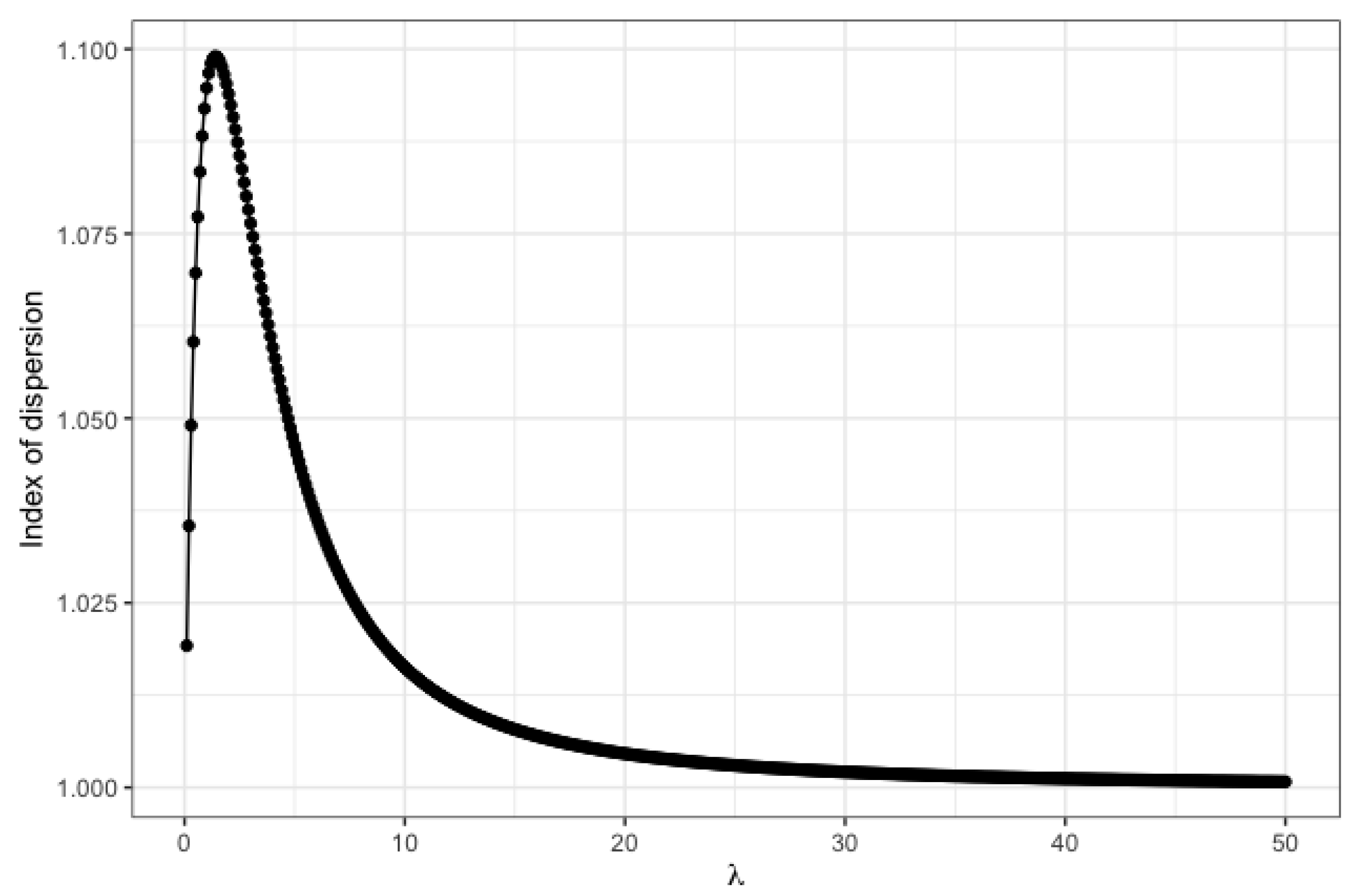
Figure 2 contains a plot showing the value of the index of dispersion for different choices of λ from 0 to 50. One can clearly note that for all values of λ , I D > 1 , which accounts for over-dispersion. For  λ = 1.4 , I D attains the maximum value of 1.099 . Additionally, as  λ approaches , the  S P distribution becomes more equi-dispersed as it approaches the standard Poisson situation.

Incomplete Moments

Incomplete moments prove to be useful in many practical problems, such as to compute the expected losses, or in relation to some characterization problems. The rth incomplete moment for a random variable X is given by,
μ r ( m ) = x = 0 m x r f ( x ) ,
where f ( x ) denotes the pmf of the random variable X, whereas, the rth incomplete factorial moment is obtained as follows:
μ [ r ] ( m ) = x = r m x [ r ] f ( x ) , m r .
Ref. [14] proposed a class of discrete distributions known as the modified power series distributions (MPSD). The form of the MPSD class is obtained as follows:
P θ ( X = x ) = a ( x ) g ( θ ) x f ( θ ) , x T ,
where θ is the underlying parameter, g ( θ ) , f ( θ ) are positive, finite and differentiable functions of θ alone, T is a subset of the set of non-negative integers, and  a ( x ) > 0 . One can note that the S P ( λ ) model is part of this family as follows:
a ( x ) = ( x + 1 ) ( x + 2 ) x ! , g ( λ ) = λ , f ( λ ) = 1 λ 2 C λ .
Hence, by utilizing the ideas from [14], one can easily derive the following recurrence relations:
μ r + 1 ( m ) = λ d d λ ( μ r ( m ) ) + μ 1 μ m ( t ) .
μ [ r + 1 ] ( m ) = λ d d λ ( μ [ r ] ( m ) ) + μ [ r ] ( m ) ( μ [ 1 ] r ) ,
where μ 1 and μ [ 1 ] are equal, and represent the mean of the S P ( λ ) distribution.

2.4. Reliability Properties

A probability distribution is said to be log-concave if its pmf satisfies the inequality P ( x ; λ ) 2 P ( x 1 ; λ ) P ( x + 1 ; λ ) , for all x, where P ( x ; λ ) denotes the pmf of a distribution. The log-concavity (log-convexity) of a distribution has an effect on the characteristic of its reliability function, failure rate function, tail probabilities and moments. Therefore, the log-concavity (log-convexity) produces an increasing failure rate (IFR) (decreasing failure rate (DFR)) and a monotonically decreasing mean residual life (DMRL) time function (increasing mean residual life (IMRL) time function), See [15]. The next proposition shows the log-concavity of the S P distribution.
Proposition 1.
If X  SP ( λ ) , then the pmf of the random variable X is log-concave for all λ and x, which is independent of λ.
Proof. 
A pmf P ( x ; λ ) is said to be log-concave if it satisfies the following inequality:
P ( x ; λ ) 2 P ( x 1 ; λ ) P ( x + 1 ; λ ) ,
for all x. For the SP model, upon utilizing the pmf from (1), the inequality above takes the form:
C λ 2 x + 1 2 λ 2 ( x + 2 ) x + 2 2 ( x ! ) 2 C λ x 2 λ x + 1 ( x + 1 ) ( x 1 ) ! × C λ ( x + 2 ) 2 λ x + 3 ( x + 3 ) ( x + 1 ) ! ,
which upon simplification gives,
( x + 3 ) ( x + 1 ) 4 > x 2 ( x + 2 ) 3 .
Hence,
3 + 13 x + 22 x 2 + 18 x 3 + 7 x 4 + x 5 > 8 x 2 + 12 x 3 + 6 x 4 + x 5 .
And thus,
3 + 13 x + 14 x 2 + 6 x 3 + x 4 > 0 ,
which indicates that the distribution portrays log-concavity and implies reliability class IFR and DMRL for all values of x, as per [15].    □
Corollary 1.
The following results are the direct consequence of log-concavity:
i 
Using the relationships between log-concavity and unimodality presented in [16], the S P distribution is unimodal.
ii 
SP is an IFR.
iii 
Convolution of SP with any other discrete distribution will also result in a log-concave distribution.
iv 
SP has at most an exponential tail, lim x e b x P ( Y = x ) = 0 , which implies P ( Y = x ) = o ( e b x ) for some b > 0 as x .
v 
SP has a monotonically decreasing mean residual life (MRL) time function.

2.5. Entropy

We derive the expansion of the Shannon entropy for the S P distribution. The Shannon entropy is defined by E [ log p ( x ) ] , where p ( x ) is the pmf of the underlying distribution. In this regard, we make use of the first characterization given in (3). Using the pmf given in (3), the Shannon entropy for the S P distribution can be written as follows:
E [ log p ( x ) ] = E [ log ( λ 2 e λ C λ ) ] + E log x + 1 x + 2 + E [ log p ( x , λ ) ] ,
where p ( x , λ ) denotes the pmf of a standard Poisson distribution with parameter λ . Now, by utilizing the Taylor series expansion for the log function and simplifying, we obtain
E [ log p ( x ) ] = log ( λ 2 e λ C λ ) E r = 1 ( 1 ) r 1 x r r + E r = 1 ( 1 ) r 1 x r 2 r r + log 2 + E [ log p ( x , λ ) ] .
Now, the last term in the equation above provides the Shannon entropy for a standard Poisson distribution, denoted as H; by using the method presented in [17], H can be approximated by
H = 1 2 log ( 2 π e λ ) 1 12 λ + O ( λ 2 ) ,
where O represents the order of λ 2 . Hence, the entropy for S P can be simplified to
E [ log p ( x ) ] = log ( λ 2 e λ C λ ) E r = 1 ( 1 ) r 1 x r r + E r = 1 ( 1 ) r 1 x r 2 r r + log 2 + 1 2 log ( 2 π e λ ) 1 12 λ + O ( λ 2 ) .

2.6. Infinite Divisibility and Further Properties

For infinite divisibility, self-decomposability and the stability property of S P ( λ ), it is noted that according to [18,19], a necessary condition for infinite divisibility of a discrete distribution P ( x ; λ ) is that P ( 0 ; λ ) > 0 , which is satisfied by the S P distribution. Moreover, classes of self-decomposable and stable distributions are subclasses of infinitely divisible distributions, therefore, S P is an infinitely divisible distribution, self-decomposable and stable.

3. Estimation

In this section, we derive the maximum likelihood estimator for the unknown parameter λ under the S P distribution. Let x 1 , x 2 , , x n be the observed values of a random sample of size n from the S P ( λ ) distribution. The corresponding likelihood and log-likelihood functions can be written as follows:
L ( λ | x 1 , x 2 , , x n ) = C λ n λ i = 1 n ( x i + 2 ) i = 1 n x i + 1 x i + 2 1 x i !
and
ln L ( λ | x 1 , x 2 , , x n ) = n ln C λ + i = 1 n ( x i + 2 ) ln λ + i = 1 n ln x i + 1 x i + 2 1 x i ! ,
respectively. By differentiating the log-likelihood from Equation (17) with respect to λ and equating to 0, one can get the MLE ( λ ^ ) using the standard approach. This equation takes the following form:
d ln L d λ = n C λ d C λ d λ + 1 λ i = 1 n ( x i + 2 ) = 0 .
The following proposition states the existence of real-valued roots for the earlier equation:
Proposition 2.
Let d ln L / d λ be denoted as D λ . Then, D λ has at least one real-valued root.
Proof. 
D λ can be simplified as follows:
D λ = n λ ( λ + 1 ) e λ C λ + 1 λ i = 1 n ( x i + 2 ) .
Thus, upon applying the L-Hospital’s rule, we obtain lim λ 0 D λ = and lim λ D λ = n < 0 . Thus, D λ crosses the x axis at least once; hence, D λ = 0 has at least one real-valued root.    □
However, since this equation is non-linear, one has to resort to a numerical approximation method to obtain the MLE. Here, we find the MLE using the “optim” function in R [20], which uses Nelder–Mead approximation. Further, according to the regularity conditions described in [21], the derived MLE has a normal distribution with the mean λ and variance provided by the following expression:
V ( λ ^ ) E λ d 2 d λ 2 ln L ( λ | X 1 , X 2 , , X n ) λ = λ ^ .

4. Simulations

In this section, we present extensive simulation analyses highlighting the performance of the maximum likelihood estimator, which is found using the approximation method. A brief overview of the underlying simulation study is provided as follows:
  • In order to generate a random sample from the S P ( λ ) distribution, we make use of the characterization based on the weighted Poisson distribution, as seen in Equation (3). We therefore generate 10,000 samples of size n from the S P ( λ ) distribution for two specific values of λ , i.e., 0.5 and 2.
  • The MLEs for a particular λ are then computed from these 10,000 samples. Let these be denoted by λ ^ i , i = 1 , 2 , , 10 , 000 .
  • Using the MLEs from step (2), we compute the biases (Biases) and mean squared errors (MSEs) of the estimates using the following forms:
    B i a s ( λ ^ , n ) = 1 10000 i = 1 10000 ( λ ^ i λ ) ,
    M S E ( λ ^ , n ) = 1 10000 i = 1 10000 ( λ ^ i λ ) 2 .
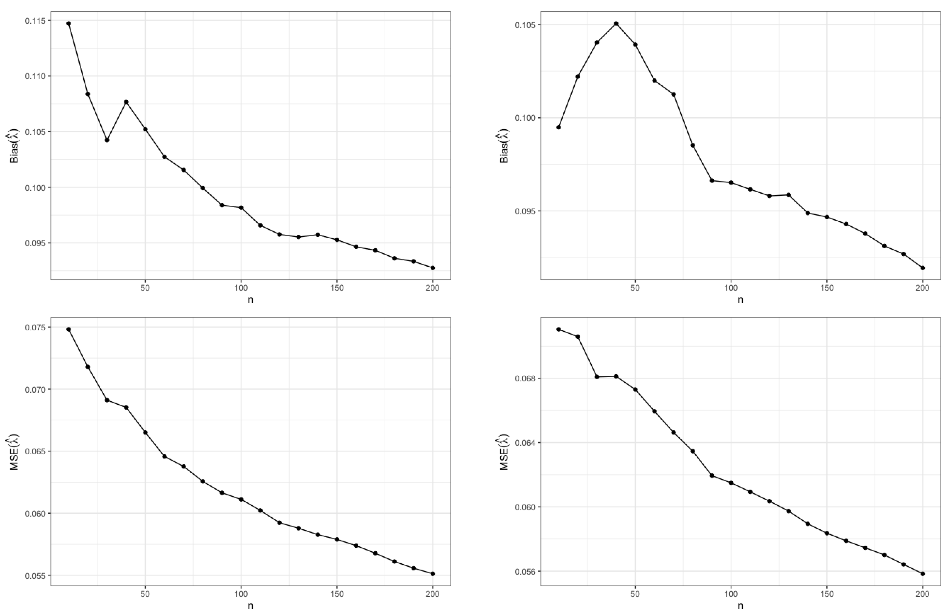
We repeat the steps above for several equidistant values of n ranging from 10 to 200. Under each combination, we find the values of the Bias and MSE. Figure 3 shows the behaviour of the Bias and MSE with respect to n for the MLE λ ^ .
Based on the plots above, one can clearly see that the Biases and the MSEs decay sharply to 0, as  n for both the parameter values. This supports the asymptotic consistency of the MLE found using the numerical approximation technique. For convenience, we present a short version of the underlying R code in the Appendix A. Users may change the parameter values to obtain the desired results.

5. Applications to Real Data

In this section, we outline the applicability of the proposed S P distribution on two real-life datasets concerning insurance claims and parasite counts. We picked these two specific examples as they show zero-inflation and over-dispersion. Zero-inflation occurs in decreasing order, from the first dataset to the second.

5.1. Dataset 1

The first dataset that we consider provides information on an infection produced by a parasite called “Trypanosoma murmanensis” in cod; the dataset has been collected over three successive years along the Finnmark coast (northern Norway). The response variable is the number of parasites found in the cods (Intensity). The dataset has been extracted from the package “countreg” of the R software, which is introduced by [22]. For completeness, we present the dataset in a frequency format in Table 1. The mean and variance of the parasite intensity happen to be μ = 0.7220 and σ 2 = 3.4940 , respectively. One can clearly note that the observations possess over-dispersion, since the variance exceeds the mean. Additionally, zero-inflation is predominant as the frequency of absence of parasites is substantial.
We now fit the S P ( λ ) distribution to the intensities. The estimated parameter is found using the maximum likelihood method, which turns out be 0.7220 . The MLE is found out using the “Brent” method in the ‘optim’ function in R. As per the Kolmogorov–Smirnov (K-S) test, the p-value is 0.71, which confirms the S P fit. This is also supported by Figure 4 that contains the S P pmf fit and the empirical distribution function (ecdf) fit.
For comparison purposes, we consider a set of comparable models, some of which are studied and compared in [23,24]. We also consider a recent zero-inflated distribution called the zero inflated Waring distribution, which is introduced by [25]. The following list contains the corresponding pmfs of these distributions:
  • ZIW (zero inflated Waring distribution) given by [25],
    P ( x ; α , β , π ) = π + ( 1 π ) α α + β , if x = 0 ( 1 π ) α ( α + β 1 ) ! ( x + β 1 ) ! ( β 1 ) ! ( x + α + β ) ! , if x > 0 ,
    where α , β > 0 and 0 π 1 .
  • NLD (new logarithmic distribution) given by [26],
    p x = log ( 1 α θ n ) log ( 1 α θ x + 1 ) log ( 1 α ) , x = 0 , 1 , 2 ,
    where α < 1 , α 0 , 0 < θ < 1 .
  • NGDP (new geometric discrete Pareto distribution), as proposed by [23],
    p x = q x ( x + 1 ) α q x + 1 ( x + 2 ) α , x = 0 , 1 , 2 ,
    where 0 < q 1 , α 0 .
  • DGP (discrete generalized Pareto), provided by [27],
    p x = 1 ( 1 + λ x ) α 1 ( 1 + λ ( x + 1 ) ) α , x = 0 , 1 , 2 ,
    where λ , α > 0 .
  • PIG (Poisson inverse Gaussian distribution), outlined by [28],
    p x = 1 x ! 2 ϕ π e ϕ / μ ϕ 1 4 + x 2 2 + ϕ μ 2 1 2 x 4 K x 1 2 2 ϕ + ϕ 2 μ 2 , x = 0 , 1 , 2 ,
    where ϕ , μ > 0 and K a ( . ) represent the modified Bessel function of the third kind with a R .
  • NB (negative binomial distribution),
    p x = ( x + r 1 ) ! x ! ( r 1 ) ! p x ( 1 p ) x x = 0 , 1 , 2 ,
    where r > 0 , 0 < p < 1 .
  • PLD (Poisson Lindley distribution) provided in [29],
    p x = θ 2 ( x + θ + 2 ) ( θ + 1 ) x + 3 x = 0 , 1 , 2 ,
    where θ > 0 .
Table 2 presents the comparison findings. One can clearly note that the proposed S P ( λ ) distribution fits the data better than the rest in terms of the log-likelihood function, AIC (Akaike’s information criterion), and BIC (Bayesian information criterion) values, and the K-S test statistic and p-value. Among AIC and BIC, one may prefer the BIC criterion, as it penalizes adding any extra parameters to the distribution. Thus, distributions that depend on more than two parameters have a tendency to be penalized.

5.2. Dataset 2

The second dataset under consideration represents the vaccine-adverse event counts and the number of claims in automobile insurance. One may refer to [30] for a further description and analysis of the dataset. Table 3 details the entire dataset in a frequency-type setting. We find that the mean and variance of the insurance claims data are μ = 1.5069 and σ 2 = 2.9034 , respectively. This clearly shows that the observations are over-dispersed.
The S P distribution is fitted on this dataset using the MLE as the estimated parameter, which is found to be λ ^ = 1.5069 . The corresponding K-S test provides a p-value of 0.58, which suggests a good fit. This is also seen in Figure 5 through the pmf fit and ecdf plots.
As a comparison, we again consider a subset of the above outlined models, along with the zero inflated Poisson (ZIP) distribution, and find the associated likelihood, AIC, and BIC values, as well as the K-S test statistics and corresponding p-values of the distribution fits. The results are displayed in Table 4. Clearly, the  S P distribution proves to be better than the other comparable models, according to all the criteria. Interestingly, it outperforms the recently introduced zero-inflated Waring distribution and the ZIP distribution.

6. Conclusions

In this paper, we proposed a flexible single-parameter discrete distribution based on a non-negative set of integers. This distribution is a weighted version of the Poisson distribution, but proves to be much better at handling over-dispersion and zero-inflation. A set of theoretical properties, such as its distribution function, characteristic function, index of dispersion, regular moments, recurrence relation of the moments, and incomplete moments, are derived. Parameter estimation is undertaken using the maximum likelihood approach. This distribution is then compared with a set of other comparable models to fit two real-life datasets related to insurance claims and parasite counts, where it is found to be superior to the rest of the models according to standard criteria.

Author Contributions

Conceptualization, H.S.B.; Methodology, S.R.B. and H.S.B.; Formal analysis, S.R.B., F.E.A. and A.M.A.; Investigation, S.R.B. and H.S.B.;Writing—original draft, S.R.B.; Writing—review & editing, F.E.A. and A.M.A. All authors have read and agreed to the published version of the manuscript.

Funding

This research was funded by Deanship of Scientific Research, Vice Presidency for Graduate Studies and Scientific Research, King Faisal University, Saudi Arabia [Grant No. 2540].

Data Availability Statement

The paper includes the data that was used in the study.

Acknowledgments

This work was supported by the Deanship of Scientific Research, Vice Presidency for Graduate Studies and Scientific Research, King Faisal University, Saudi Arabia [Grant No. 2540].

Conflicts of Interest

The authors declare no conflict of interest.

Appendix A. R Codes

x<-c()
y<-c()
b_l<-c()
mse_l<-c()
for(n in seq(from=10, to=200, by=10)){
  l=0.5
  for(i in 1:1000){
    nll <- function(lam) {
      c<-lam^2/(exp(lam) ∗ (lam^2-lam+1)-1)
      z<-rpois(n,l)
      -n ∗ log(c)-sum(log((z+1)/(z+2) ∗ /factorial(z)))
      -sum(z) ∗ log(lam)+n ∗ lam
    }
fit<-optim(l<-c(2),nll,hessian = FALSE)
x<-c(x,fit$par[1])
  }
  b_l<-c(b_l,mean(x)-l)
  mse_l<-c(mse_l,mean((x-l)^2))
}
 
df<-data.frame(b_l,mse_l)
 
n=seq(from=10, to=200, by=10)
ggplot(data=df, aes(x=n, y=b_l))+
  geom_line()+
  geom_point()+
  xlab("n")+
  ylab(expression(Bias(hat(lambda))))+
  theme_bw()

References

  1. Lambert, D. Zero-Inflated Poisson regression, with an application to defects in manufacturing. Technometrics 1992, 34, 1–14. [Google Scholar] [CrossRef]
  2. Böhning, D.; Dietz, E.; Schlattmann, P.; Mendonca, L.; Kirchner, U. The zero-inflated Poisson model and the decayed, missing and filled teeth index in dental epidemiology. J. R. Stat. Soc. Ser. A 1999, 162, 195–209. [Google Scholar] [CrossRef]
  3. Atkins, D.C.; Gallop, R.C. Rethinking how family researchers model infrequent outcomes: A tutorial on count regression and zero-inflated models. J. Fam. Psychol. 2007, 21, 726–735. [Google Scholar] [CrossRef]
  4. Fagundes, R.A.A.; Souza, R.M.C.R.; Cysneiros, F.J.A. Zero-inflated prediction model in software-fault data. IET Softw. 2016, 10, 1–9. [Google Scholar] [CrossRef]
  5. Greene, W.H. Accounting for Excess Zeros and Sample Selection in Poisson and Negative Binomial Regression Models. NYU Working Paper No. EC-94-10. 1994. Available online: https://papers.ssrn.com/sol3/papers.cfm?abstract_id=1293115 (accessed on 17 January 2023).
  6. Mullahy, J. Specification and testing of some modified count data models. J. Econom. 1986, 33, 341–365. [Google Scholar] [CrossRef]
  7. Bandyopadhyay, D.; DeSantis, S.M.; Korte, J.E.; Brady, K.T. Some considerations for excess zeroes in substance abuse research. Am. J. Drug Alcohol Abus. 2011, 37, 376–382. [Google Scholar] [CrossRef] [PubMed]
  8. Coxe, S.; West, S.G.; Aiken, L.S. The analysis of count data: A gentle introduction to Poisson regression and its alternatives. J. Personal. Assess. 2009, 91, 121–136. [Google Scholar] [CrossRef]
  9. Hu, M.; Pavlicova, M.; Nunes, E.V. Zero-inflated and hurdle models of count data with extra zeros: Examples from an HIV-risk reduction intervention trial. Am. J. Drug Alcohol Abus. 2011, 37, 367–375. [Google Scholar] [CrossRef] [Green Version]
  10. Usman, M.; Oyejola, B.A. Models for count data in the presence of outliers and/or excess zero. Math. Theory Model. 2013, 3, 94–103. [Google Scholar]
  11. Tüzen, M.F.; Erbaş, S. A comparison of count data models with an application to daily cigarette consumption of young persons. Commun. Stat.-Theory Methods 2018, 47, 5825–5844. [Google Scholar] [CrossRef]
  12. Louzayadio, C.G.; Malouata, R.O.; Koukoutikissa, M.D. A weighted Poisson distribution for underdispersed count data. Int. J. Stat. Probab. 2021, 10, 157. [Google Scholar] [CrossRef]
  13. Rattihalli, R.N.; Bhati, D. Generation of new families of discrete distributions. Calcutta Stat. Assoc. Bull. 2017, 68, 135–146. [Google Scholar] [CrossRef]
  14. Tripathi, R.C.; Gupta, P.L.; Gupta, R.C. Incomplete moments of modified power series distributions with applications. Commun. Stat.-Theory Methods 1986, 15, 999–1015. [Google Scholar] [CrossRef]
  15. Gupta, P.L.; Gupta, R.C.; Tripathi, R.C. On the monotonic properties of discrete failure rates. J. Stat. Plan. Inference 1997, 65, 255–268. [Google Scholar] [CrossRef]
  16. Grandell, J. Mixed Poisson Processes; Chapman & Hall: London, UK, 1997. [Google Scholar]
  17. Evans, R.J. Ramanujan’s Second Notebook: Asymptotic expansions for hypergeometric series and related functions. In Ramanujan Revisited; Academic Press: New York, NY, USA, 1988. [Google Scholar]
  18. Nekoukhou, V.; Alamatsaz, M.H.; Bidram, H. A discrete analog of the generalized exponential distribution. Commun. Stat.-Theory Methods 2012, 41, 2000–2013. [Google Scholar] [CrossRef]
  19. Steutel, F.W.; van Harn, K. Infinite Divisibility of Probability Distributions on the Real Line, 1st ed.; CRC Press: Boca Raton, FL, USA, 1979. [Google Scholar]
  20. R Core Team. R: A Language and Environment for Statistical Computing; R Foundation for Statistical Computing: Vienna, Austria, 2022; Available online: https://www.R-project.org/ (accessed on 17 January 2023).
  21. Rohatgi, V.K.; Saleh, A.K. An Introduction to Probability and Statistics, 2nd ed.; John Wiley and Sons: Hoboken, NJ, USA, 2000. [Google Scholar]
  22. Zeileis, A.; Kleiber, C. Countreg: Count Data Regression. R Package Version 0.2-0. 2018. Available online: http://R-Forge.Rproject.org/projects/countreg/ (accessed on 17 January 2023).
  23. Bhati, D.; Bakouch, H.S. A new infinitely divisible discrete distribution with applications to count data modeling. Commun. Stat.-Theory Methods 2019, 48, 1401–1416. [Google Scholar] [CrossRef]
  24. Shaul, K.B.; Ridder, A. Exponential dispersion models for over-dispersed zero-inflated count data. Commun. Stat.-Simul. Comput. 2021. [Google Scholar] [CrossRef]
  25. Rivas, L.; Campos, F. Zero inflated Waring distribution. Commun. Stat.-Simul. Comput. 2021. [Google Scholar] [CrossRef]
  26. Gómez-Déniz, E.; Sarabia, J.M.; Calderín-Ojeda, E. A new discrete distribution with actuarial applications. Insur. Math. Econ. 2011, 48, 406–412. [Google Scholar] [CrossRef]
  27. Prieto, F.; Gómez-Déniz, E.; Sarabia, J.M. Modelling road accident blackspots data with the discrete generalized Pareto distribution. Accid. Anal. Prev. 2014, 71, 38–49. [Google Scholar] [CrossRef] [Green Version]
  28. Willmot, G. The Poisson-inverse Gaussian as an alternative to the negative binomial. Scand. Actuar. J. 1987, 3, 113–127. [Google Scholar] [CrossRef]
  29. Sankaran, M. The Discrete Poisson-Lindley Distribution. Biometrics 1970, 26, 145–149. [Google Scholar] [CrossRef]
  30. Rose, C.E.; Martin, S.W.; Wannemuehler, K.A.; Plikaytis, B.D. On the use of zero inflated and hurdle models for modeling vaccine adverse events count data. J. Biopharm. Stat. 2006, 16, 463–481. [Google Scholar] [CrossRef] [PubMed]
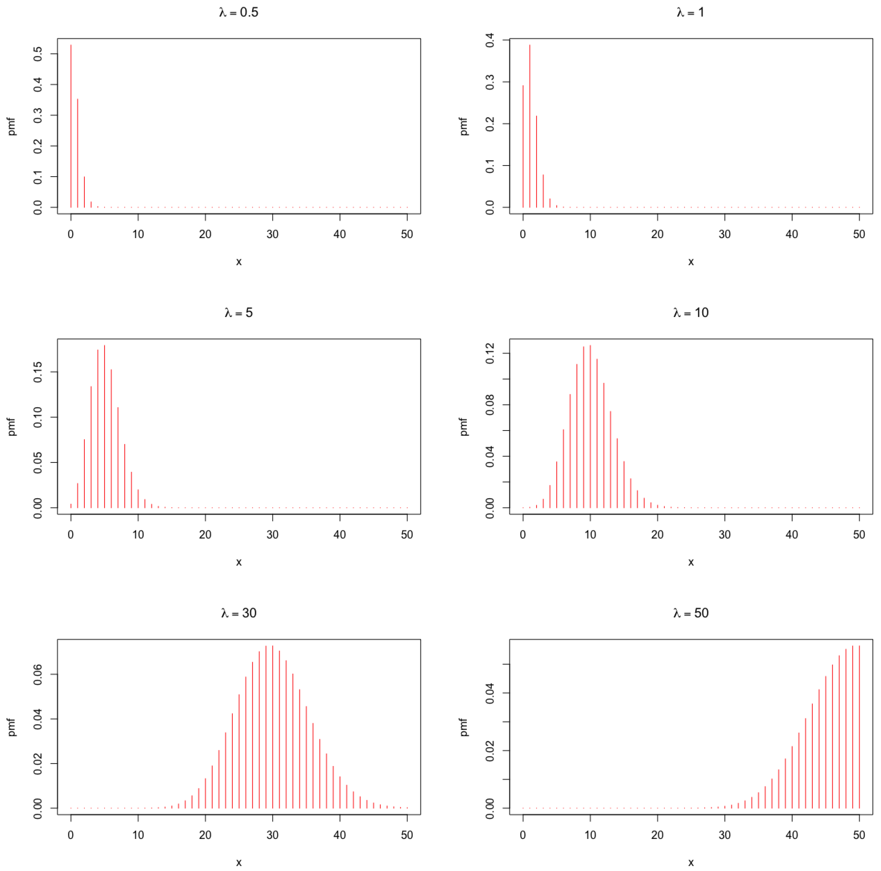
Figure 1. Pmf of the S P ( λ ) distribution for different parameter combinations.
Mathematics 11 01122 g001
Figure 2. Index of dispersion for different values of λ .
Mathematics 11 01122 g002
Figure 3. Bias and MSE for λ = 0.5 (left) and λ = 2 (right).
Mathematics 11 01122 g003
Figure 4. Fitted pmf plot (left) and ecdf plot (right) for the parasite intensity data.
Mathematics 11 01122 g004
Figure 5. Fitted pmf plot (left) and ecdf plot (right) for the insurance claims data.
Mathematics 11 01122 g005
Table 1. Parasite intensity data.
Value012345678910
Frequency65438332117121110548
Table 2. Comparing model fits for the parasite intensity data.
ModelFitted ParametersLog-LAICBICK-Sp-Value
SP  ( λ ) λ ^ = 0.7220 −778.181558.361563.060.040.71
Poisson  ( λ ) λ ^ = 0.7130 −1332.852667.712672.410.240.04
ZIW  ( α , β , π ) α ^ = 1.04 , β ^ = 0.26 , −781.561569.121583.220.050.64
π ^ = 0.49
NLD  ( α , θ ) α ^ = 0.55 , θ ^ = 0.17 −824.191652.381661.780.180.13
NGDP  ( q , α ) q ^ = 0.73 , α ^ = 5.92 −800.911605.681615.080.110.36
DGP  ( λ , α ) λ ^ = 0.71 , α ^ = 5.38 −811.121626.241655.640.150.26
PIG  ( ϕ , μ ) ϕ ^ = 0.052 , μ ^ = 0.108 −791.541587.821596.480.210.42
NB  ( r , p ) r ^ = 0.58 , p ^ = 0.32 −785.411574.821584.220.080.51
PLD  ( θ ) θ ^ = 1.92 −974.371950.741955.450.060.06
Table 3. Insurance claims data.
Value0123456789101112
Frequency143710106604282361226234148441
Table 4. Comparing model fits for the insurance claims data.
ModelFitted ParametersLog-LAICBICK-Sp-Value
SP  ( λ ) λ ^ = 1.50 −3753.6277149.297155.540.040.58
Poisson  ( λ ) λ ^ = 1.51 −7231.1314,464.2714,470.570.290.05
ZIW  ( α , β , π ) α ^ = 48.92 , β ^ = 67.02 −6797.2513,588.5113,619.410.180.24
π ^ = 0.45
ZIPD  ( μ , σ ) μ ^ = 2.04 , σ ^ = 0.26 −6869.5513,741.513,754.10.240.22
NGDP  ( q , α ) q ^ = 0.51 , α ^ = 0.33 −6741.7813,487.5713,500.160.100.33
NB  ( r , p ) r ^ = 1.52 , p ^ = 0.50 −6741.613,485.213,486.330.060.44
PLD  ( θ ) θ ^ = 0.99 −6745.9913,493.9913,500.290.140.29
Disclaimer/Publisher’s Note: The statements, opinions and data contained in all publications are solely those of the individual author(s) and contributor(s) and not of MDPI and/or the editor(s). MDPI and/or the editor(s) disclaim responsibility for any injury to people or property resulting from any ideas, methods, instructions or products referred to in the content.