Abstract
Recently, a swarm-based method called Artificial Hummingbird Algorithm (AHA) has been proposed for solving optimization problems. The AHA algorithm mimics the unique flight capabilities and intelligent foraging techniques of hummingbirds in their environment. In this paper, we propose a modified version of the AHA combined with genetic operators called mAHA. The experimental results show that the proposed mAHA improved the convergence speed and achieved better effective search results. Consequently, the proposed mAHA was used for the first time to find the global maximum power point (MPP). Low efficiency is a drawback of photovoltaic (PV) systems that explicitly use shading. Normally, the PV characteristic curve has an MPP when irradiance is uniform. Therefore, this MPP can be easily achieved with conventional tracking systems. With shadows, however, the conditions are completely different, and the PV characteristic has multiple MPPs (i.e., some local MPPs and a single global MPP). Traditional MPP tracking approaches cannot distinguish between local MPPs and global MPPs, and thus simply get stuck at the local MPP. Consequently, an optimized MPPT with a metaheuristic algorithm is required to determine the global MPP. Most MPPT techniques require more than one sensor, e.g., voltage, current, irradiance, and temperature sensors. This increases the cost of the control system. In the current research, a simple global MPPT method with only one sensor is proposed for PV systems considering the shadow conditions. Two shadow scenarios are considered to evaluate the superiority of the proposed mAHA. The obtained results show the superiority of the proposed single sensor based MPPT method for PV systems.
Keywords:
modified artificial hummingbird algorithm; metaheuristics; maximum power point tracking; single sensor MSC:
68T99; 68U99
1. Introduction
Optimization is used to solve many problems by maximizing or minimizing objective functions. Various optimization methods are used to find the optimal solution. Metaheuristic algorithms (MHs) are optimization tools in which various methods are used to increase the effectiveness of search processes [1,2,3,4]. Although it is difficult to find an exact solution in most cases, algorithms can provide the optimal global solution [5].
In this context, MHs can be divided into two categories: stochastic and deterministic methods. If the gradient is available, deterministic algorithms could be an option. Since these different techniques are based on established computations, it can be assumed that the optimization procedure is repeatable. Each time the algorithm is run with the same initial conditions, the optimization path and result are identical, making the process replicable. Stochastic methods, on the other hand, have random properties that generate different optimization pathways, leading to different optimized solutions even if the initial conditions are the same for each run. The main advantage of stochastic algorithms is that they do not require gradient information. However, accessing gradient information is becoming increasingly difficult as problems become more complex. Researchers have developed stochastic algorithms that do not require gradient information. The category of MHs was developed due to the advancement of stochastic techniques [6]. Some stable MHs, including genetic algorithm (GA) [7], particle swarm optimization (PSO) [8], bee colony optimization (BCO) [9], and differential evolution [10], have been used to solve various optimization problems. For example, MHs have excelled in several real-world applications, such as medicine [11,12], COVID-19 [13,14], feature selection [15,16], and image segmentation [17], as well as combinatorial problems [18,19,20].
Recently, an efficient swarm-based method called artificial hummingbird algorithm (AHA) has been proposed for solving optimization problems [21]. The source of inspiration of AHA is to mimic the unique flight capabilities and intelligent foraging behavior of hummingbirds in their environment. Although AHA has been used to solve various optimization problems, AHA still suffers from some drawbacks, such as (1) fast convergence and robust utilization of space, (2) fast convergence to the found optimal solution, (3) lack of self-adaptation of convergence rate. The aforementioned drawbacks cause the algorithm to fall victim to the problem of premature convergence, which leads to further problems, such as the algorithm getting stuck in regions with local optima, which prevents it from finding the nearest/best solutions.
In this paper, the genetic operators are combined with the original AHA algorithm to propose a modified version called mAHA. The role of genetic operators is to drive the solution from local to global to improve the position and enable trapping in local search, increasing the diversity of algorithms and avoiding local solutions in the comparison between a new and a previous solution. The mAHA was used to solve the IEEE CEC’20 test suite for optimization testing, and the results were compared with several stable methods, including SMA [22], HHO [23], GWO [24], WOA [25], and the original AHA [21]. The experimental results show that the proposed mAHA achieves (1) effective search results, (2) lower computational cost, (3) good convergence speed, (4) balanced exploration and exploitation behavior, and (5) avoidance of local optimum.
Electric power generation has been driven by new and renewable energy sources (RES), which have seen rapid growth in the energy industry in recent years. Their ability to provide clean, renewable, maintenance-free, ubiquitous, and low-cost energy has increased the popularity of renewable energy [26]. Moreover, renewables can improve the reliability and self-healing operation of utility grids through their reconfiguration into microgrids and nanogrids. The installed capacities of renewable energy sources are increasing rapidly worldwide. Photovoltaic (PV) capacity will increase by 179 TWh in 2021, a 22% growth from 2020. It accounts for 3.6% of global electricity generation [27]. PV electricity is the third largest energy source after hydropower and wind. It is expected that PV generation will be about 7400 TWh in 2030. Tracking the maximum power point (MPP) is very important for increasing the efficiency of the PV system. Under normal conditions, i.e., uniform irradiance distribution, the power-voltage characteristic has only a single MPP [28]. This MPP can be easily extracted using conventional MPPT techniques such as incremental resistance and hill climbing. The situation is quite different for shaded conditions. Especially for large PV systems, the probability of the presence of shade due to nearby trees or buildings is very high [29]. The shadow problem reduces the PV output power. It is difficult to avoid the shading. Therefore, a bypass diode is used to mitigate the shadow and protect the PV system. During shading, the bypass diode is on and provides an additional path to current draw. However, during normal operation, the bypass diode is off and has no effect [30]. In summary, the power-voltage curve with shadow has some local MPP and one global MPP. The conventional MPP tracking approaches cannot distinguish between local and global MPPs and therefore simply stop at the local MPP. Consequently, an optimized MPPT with a metaheuristic algorithm is required to determine the global MPP. The previous algorithms that have been used to mitigate the shadow effect are the Marine Predator algorithm [31], Search & Rescue algorithms [32], Group Teaching Optimization [33], and the Firefly algorithm [34].
The disadvantage of previous techniques is that more than one sensor is needed, e.g., voltage, current, irradiance, and temperature sensors. El-Helw et al. [35] proposed a global MPPT method using a neural network that requires six sensors: four irradiance sensors, voltage, and current. Moreover, the proposed method depends on the PV module characteristics. In the same direction, Nafeh [36] proposed an MPPT method using perturbation and observation, which requires five sensors: two voltage sensors, two current sensors, and one temperature sensor. Moreover, the shadow problem was not considered. Camilo et al. [37] proposed an MPPT method based on the Monod equation. This technique requires three sensors: current, temperature and radiation. Moreover, the shadow condition is not considered. To fill the defined research gap, a global MPPT method with one sensor for PV systems is proposed in this paper. For the first time, a mAHA is proposed to mitigate the shadow and determine the global MPP in PV systems.
The contributions of the paper can be outlined as follows.
- In this paper, an effective method called mAHA is proposed.
- The proposed mAHA introduces the mechanisms of genetic operators (crossover and mutation selection) to enhance AHA’s performance in increasing the diversity of the population and avoiding local searches.
- The proposed mAHA was adopted to address the ten global optimization tasks from the CEC’20 test suite and was compared with other optimization algorithms and the original AHA algorithm.
- For the first time, a mAHA was used in the global MPPT optimization of PV systems with a sensor.
- The superiority of the proposed MPPT technique has been demonstrated.
The remaining sections are organized as follows: The artificial hummingbird algorithm (AHA) is discussed in Section 2. Section 3 discusses the proposed mAHA algorithm. Section 4 presents the evaluation results, including the CEC’20 test suite. Section 5 present the maximum power point tracking (MPPT) application results. A brief discussion is introduced in Section 6. Finally, Section 7 presents the conclusions and future work.
2. Artificial Hummingbird Algorithm
In this section, we explain the mathematical model of AHA, which is biologically inspired by the smart behavior of hummingbirds and developed to solve various optimization problems [21]. The three basic phases of the AHA algorithm is explained below:
Food sources: The hummingbird frequently evaluates the characteristics of the sources, such as the nectar quality/quantity of each nectar replenishment rate, the flowers, and the last time the flowers were visited, to select a suitable source from a group of food sources. For simplicity, it is assumed that each food source in AHA has the same type and number of flowers—the solution vector represents the food source, and the function fitness value represents the nectar fill rate. Accordingly, the higher the nectar fill rate, the better the fitness value.
Hummingbirds: each hummingbird has a specific food source from which it can only feed, so the food source and the hummingbird are constantly in the same place. The hummingbird can register the location and nectar replenishment of a particular food source and pass this knowledge on to other hummingbirds throughout the population. In addition, each hummingbird could remember how long ago it last visited a particular food source.
Visit table: for different hummingbirds, the visit frequency for each food source is recorded in the visit table and indicates how long it has been since the same hummingbird visited a particular food source. For a hummingbird, the food source with the highest visitation rate is prioritized for visitation. To obtain more nectar, among the food sources, a hummingbird should visit the one that has the highest nectar replenishment rate with the same highest visitation level. Moreover, the visitation table is updated at each iteration to find the target food source.
Moreover, the mathematical phases of the three foraging behaviors of hummingbirds including the following phases: (1) guided foraging, (2) territorial foraging, and (3) migrating foraging are discussed in the following subsections. In Algorithm 1, the generic AHA structure is provided [21].
| Algorithm 1: Structure of AHA. |
| Initialization While stop criterion is not satisfied Guided foraging Territorial foraging Migration foraging End |
2.1. The Mathematical Model of AHA Algorithm
2.1.1. Initialization Phase
The food sources construct the population of hummingbirds, and is initialized randomly as defined in [38] by Equation (1):
where for -Dim problem, the Low and represent the upper and lower boundaries. The variable is a random vector within , and the th food source position is represented by which is the solution of a specific problem. Accordingly, the visit table is defined by Equation (2):
where for null refers to hummingbird is taking food from its particular food source; for , refers to th food source that has just been visited by the th hummingbird in this current iteration.
2.1.2. Guided Foraging Phase
By incorporating a direction-switching vector into the AHA algorithm, three flight capabilities are used as follows: omnidirectional, diagonal, and axial flights are appropriately described during foraging. This vector is used to regulate the availability of one or more directions in a dimension space. Axial flight shows that hummingbirds can fly along any coordinate axis, while diagonal flight, which is determined by any two of three axes, allows hummingbirds to fly from one corner of the rectangle to the other.
To be specific, all three flight patterns can be adapted to d-Dim, where axial flying is formulated by Equation (3) as:
Moreover, diagonal flight is formulated by Equation (4) as:
Then, omnidirectional flight is formulated by Equation (5) as:
where ([1, d]) produces randomly an integer within 1 and d, a random integer permutation within 1 and k is generated by the (k), and r1 is a random number within (0, 1]. Diagonal flight in a d-Dim is placed within a hyperrectangle that is bound by any 2 to d-1coordinate axes.
Moreover, the mathematical modelling for the guided foraging behavior and candidate food source is defined as follows:
where the th food source position at time is represented by . The target food source at th hummingbird is represented by , the variable is a guided factor with mean equal 0 and standard deviation equal 1.
Accordingly, the position of th food source is updated as follows:
where the function fitness value is indicated by . The AHA’s guided foraging method is presented in Algorithm 2 [21].
| Algorithm 2: Guided foraging strategy of AHA. |
2.1.3. Territorial Foraging Phase
The local search within territorial foraging phase and the candidate food source is defined by the mathematical formula:
where the territorial factor is a normal distribution , represented by b with mean equal 0 and standard deviation equal 1. The territorial foraging phase of AHA algorithm is reported in Algorithm 3 [21].
| Algorithm 3: Territorial foraging strategy of AHA. |
| For th hummingbird from 1 to |
| Perform Equation |
| If |
| For th food source from 1 to |
| Visit_table Visit_table |
| End |
| For th food source from 1 to |
| Visit_table max Visit_table |
| End |
| Else |
| For th food source from 1 to |
| Visit_table Visit_table |
| End |
| End |
| End |
2.1.4. Migration Foraging Phase
Randomly, from the source, the obtained migration foraging with the lowest nectar-refilling rate to a new one is defined as:
where the food source is represented by in the population with the lowest nectar-refilling rate. Moreover, the migration foraging phase of AHA algorithm is reported in Algorithm 4 [21].
| Algorithm 4: Migration foraging strategy of AHA. |
| If |
| Perform Equation (11) |
| For th food source from 1 to |
| Visit_table wor, Visit_table wor, |
| End |
| For th food source from 1 to |
| Visit_table , worVisit_table |
| End |
| End |
In AHA, the following formula is used to define the migration coefficient in relation to population size as follows:
3. The Proposed mAHA Algorithm
In this section, the AHA algorithm is combined with genetic operators with AHA algorithm to build a new version called mAHA. To be specific, the AHA includes three stages: (1) Search agents are controlled; (2) search agents are produced for the hybrid method; (3) the new population based on the previous step is updated.
In the update step, all AHA search agents control each position. Here, the genetic operators produce more populations to avoid local optimality and affect AHA positions. Creating a new hybrid search agent requires creating a new hybrid individual from the current AHA as shown in Equation (13).
where value between indicates AHA weight, is AHA position, and represents AHA individual position based on the operators, so this Equation (13) indicates the effects of them. The search agent is updated using a greedy selection to select the optimal candidate solution. To improve the quality of solutions and performance of the proposed algorithm. The reasons that motivate us to present an alternative version of AHA called mAHA algorithm are described in the following subsections.
3.1. Shortcomings of the Original AHA
Although the original AHA algorithm exhibits rapid convergence during the exploration of the optimization problem space, where the solutions in each iteration move rapidly toward the optimal solution found at the current time, this solution may not be the best for the entire problem space. Moreover, the convergence of the algorithm is not self-adjusted to encourage the proposed solutions to explore the remaining regions in the problem space, but the convergence rate of AHA is not self-adjusted, which causes the algorithm to suffer from the problem of premature convergence. This leads to other problems, such as the algorithm getting stuck in regions with local optima and not being able to identify the closest/best solutions. For complex optimization problems, the algorithm AHA, like other metaheuristic optimization methods, is unable to adequately explore the entire search space in its current state [2].
Therefore, to address these drawbacks of AHA, this paper proposes an alternative version called modified artificial hummingbird algorithm (mAHA) by integrating the genetic operator’s techniques. Genetic operators control the solution from local to global using Equations (15) and (20) to enhance the position and permit the trapping in local search, thereby increasing the variety of algorithms and avoiding local solutions compared between a new and previous one. For more diversity, genetic algorithm operators are used to integrate two mutant vectors, namely and , to generate a new child as described in Equation (19). Offspring fitness value: , and based on the selection operator Equation (20) were compared to get the best prey . To identify the best candidate solution, the search space was boosted by exploring new regions, so several positions are updated by Equations (19) and (20). The stop condition is the maximum iterations that permit for evaluating the performance of the mAHA algorithm. Upon completing the mAHA process, the best position is returned. Algorithm 5 demonstrates how the best solution is proposed by calculating the objective function using Equation (14) for many new populations. mAHA fitness is indicated as defined as:
where and fobj , where is the greatest iteration. However, neither the algorithm performance nor the optimization problem space is affected.
Additionally, plots of convergence curves in most testing functions show a slow divergence of the original AHA during exploitation at most function evaluations, demonstrating that the approach is trapping in local rather than global regions.
3.2. Architecture of the Proposed mAHA Algorithm
The main goal of this research is to propose an efficient alternative version of the original AHA to solve the problems mentioned in the previous section. However, it improves the algorithm AHA, by increasing the exploration time and maintaining diversity using the genetic operator strategy.
The mathematical modeling and steps of the mAHA are formulated in Algorithm 5. The algorithm starts with a random starting population of size 2N. In the modified mAHA, the solutions of the population are evolved first, followed by the individual phase from the original AHA. At each iteration, a linear population reduction is applied to manage the population diversity, and the same approach is repeated until the optimization is complete. The following subsections explain the genetic operators.
Genetic Operators
Several algorithms use evolutionary operators, especially the two basic algorithms namely, differential evolution and genetic algorithms. Some examples of such operators are mutation as Bit inversion, crossover as single-point crossover and selection.
Mutation: The mutation operation is built using the results of AHA tasks, as the solution goal Position. A number between 0 and 1 is produced at random for each component. The target agent element position is considered when the value reaches the mutation rate (zeta). If this value is less than the mutation rate (zeta), the old vector is replaced with a component of the or vectors. The mutation operator is determined by applying the following formula: where dimension is known by and have D components generated by randomly between (0, 1).
Crossover: The crossover is the combination of two individuals to produce more variety. To generate a new offspring wCross, a linear combination with random integers tau and tau’ is used.
Selection: The selection type used in AHA is a greedy selection, which is based on differential evolution. When functions of evolution (mutation and crossover) are accessed, the offspring are created. The child and parent’s performance are then compared to determine which is the best. Finally, if the parent’s performance is good, then they have a chance to stay in the population. The rule that defines greedy selection is as follows:
where p(x) is the current position and () is the next position.
Eventually, the pseudo code of the proposed mAHA algorithm is given in Algorithm 5.
| Algorithm 5: The proposed mAHA. |
| 1- Initialization phase based on Equations (1) and (2) 2- While stop criterion is not satisfied 3- Calculate the fitness of all individuals the best search agent. 4- Calculate guided foraging using Algorithm 2 5- Calculate territorial foraging using Algorithm 3 6- Calculate migration foraging using Algorithm 4 7- 8- End While 9- Return the best criteria |
4. Experimental Stage 1: Statistical Results for CEC’20 Test Suite
Several metaheuristic algorithms (MHs) are applied to solve different optimization problems such as adaptive gaining sharing knowledge [39], differential evolution through Bayesian [40], adapted evolutionary algorithm [41], and the hybrid gaining-sharing knowledge [42]. In this study, the IEEE CEC’20 test suite [43] is one of the proper test metrics, as it tests the optimizer performance over ten various search spaces, the performance of the proposed mAHA is assessed over the CEC’20 test suite on Dim 10 and Dim 20. The experimental results of the proposed mAHA on the CEC’20 test suite is compared to the results obtained from set of the state-of-the-art optimization algorithms, namely the slime mold algorithm (SMA) [22], Harris hawks optimization (HHO) [23], grey wolf optimizer (GWO) [24], whale optimization algorithm (WOA) [25], and the original AHA [21].
4.1. Statistical Results Analysis
Further, the statistical metrics includes the average, and the standard deviation (STD) methods are applied for the best-so-far solutions reached in each run. Table 1 and Table 2 exhibit these statistical results for the proposed mAHA algorithm and the other competitors for each CEC’20 test suite with the Dim 10 and Dim 20 respectively. As the CEC’20 test suite are minimization problems, the best results are the lowest values. The introduced mAHA approach outperformed the other comparative algorithms in solving most of the CEC’20 test suite in terms of mean and STD. Consequently, the proposed mAHA algorithm achieved the first rank in the Friedman mean rank-sum test. Moreover, Table 3 reports the computation time that has been obtained by the proposed mAHA and the competitor algorithms for 30 runs with Dim 10 and Dim 20 on the CEC’20 test suite.

Table 1.
The statistical results on the CEC’20 test suite that have been obtained by the proposed mAHA and the competitor algorithms for 30 runs with Dim 10.
Table 2.
The statistical results on the CEC’20 test suite have been obtained by the proposed mAHA and the competitor algorithms for 30 runs with Dim 20.
Table 3.
The CPU time that has been obtained by the proposed mAHA and the competitor algorithms for 30 runs with Dim 10 and Dim 20 on the CEC’20 test suite.
4.2. Convergence Performance Analysis
The performance of the proposed mAHA and other competitors evaluated on the CEC’20 test suite, the results are explained graphically with the convergence curves as shown in Figure 1. According to the convergence plots, the proposed mAHA reached a stable point over most of the test methods. From convergence plots the fast convergence refers to the optimal solution. Thus, the introduced mAHA method considers an applicable approach to tackle different optimization problems that need fast computing i.e., the online optimization problems.
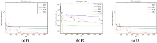
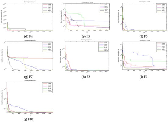
Figure 1.
The convergence curves on the CEC’20 test suite have been obtained by the proposed mAHA and the competitor algorithms for 30 runs with Dim10.
4.3. Boxplot Behavior Analysis
Boxplots are employed to exhibit the data distribution. The distribution reflects the local minimum of test functions. Furthermore, boxplots consider an effective presenting method for data distributions in quartiles, where the obtained maximum and minimum data points are represented by the Boxplot whisker’s edges. Furthermore, the higher the level of data agreement, the narrower the boxplot, Figure 2. Boxplot introduces the results for ten functions, Dim10. It is observed that the mAHA algorithm reaches the best results compared to the other algorithms.
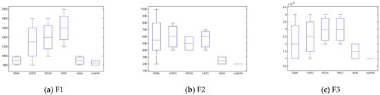
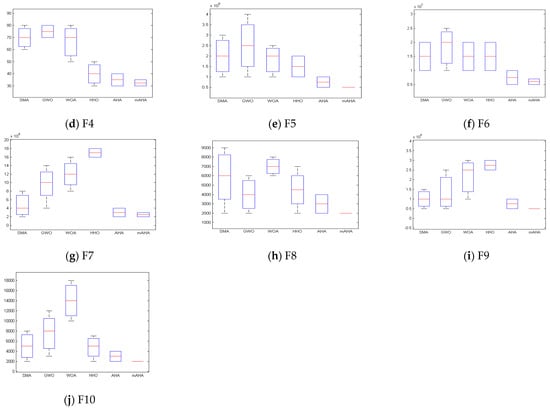
Figure 2.
The box-plot curves on the CEC’20 test suite that have been obtained by the proposed mAHA and the competitor algorithms for 30 runs with Dim10.
4.4. Qualitative Metrics Analysis
The optimizer solutions behavior reflects a stable analysis about the algorithm performance and behavior through the search process. The qualitative analysis of the proposed mAHA introduced in Figure 3, shows the agent’s behaviors, 3D views of the functions, average fitness history, search history, and convergence curves.
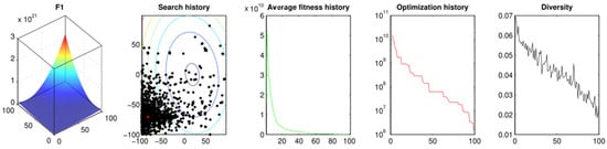
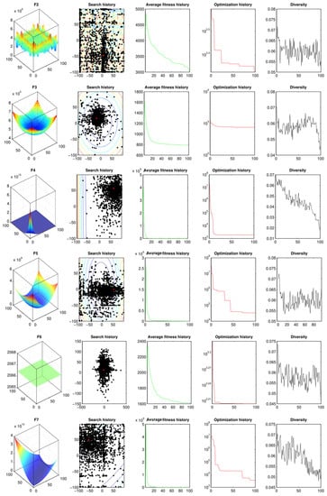
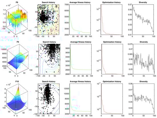
Figure 3.
The qualitative metrics on the CEC’20 test suite have been obtained by the proposed mAHA.
The next points are worthwhile from the visualization curves such as convergence, boxplots, and qualitative analysis:
- (1)
- Search history: The second column in Figure 3 shows the agents’ search history from the beginning to the last iteration. Furthermore, the problem search space is formed on a counter line, it reflects the gradient from blue to red color lines indicating a higher fitness value. The introduced mAHA approach can reach the positions with the higher fitness values, according to the search history.
- (2)
- Average fitness history: The third column in Figure 3 demonstrates the average fitness value. From this figure, the agents’ overall behavior is represented by the fitness history as well as their contribution in the optimization process.
- (3)
- Accordingly, the performance of mAHA approach is assessed against the other competitors on CEC’20 test suite. The performance of the proposed mAHA is evaluated using both quantitative and qualitative indicators for mAHA. According to Table 1, Table 2 and Table 3, the proposed mAHA method has reached near/optimal results for convergence and the highest fitness value. The graphical boxplot and minimum convergence curve are shown in Figure 1 and Figure 2 respectively. These graphical representations demonstrate the stable performance of the proposed mAHA algorithm as introduced in Figure 3, which indicate that the introduced method is dependable for a real situation and are drawn from the test metrics.
5. Stage 2: Maximum Power Point Tracking
The PV system is shown in Figure 4. It includes 36 photovoltaic panels forming 6 arrays, DC-DC converter, controller, and 480 V battery bank. The specification of the PV system is presented in Table 4.
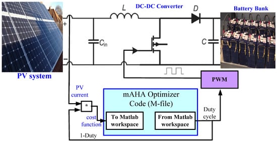
Figure 4.
Schematic diagram for PV system with MPPT.
Table 4.
Specifications of the PV system.
The duty cycle is the key to control the DC-DC converter to boost the PV power. It may be defined as follows:
where and represent the PV voltage and battery voltage respectively.
The PV voltage may be defined as follows:
where D is the duty cycle.
Referring to the above relation, with constant battery voltage, the PV voltage is proportional with (1 − D). Therefore, as an alternative of utilizing voltage sensor, it can be using the value of (1 − D) to replace the PV voltage. Consequently, the objective function required to be maximum can be defined as follows.
where IPV denotes PV current, and the duty cycle (D) is selected to be the decision variable during the optimization process.
Two shadow scenarios have been considered to assess the suggested mAHA global MPPT technique. Figure 5 and Table 5 show the PV characteristics of the two scenarios. Altering shadow pattern is conducted to change the location of global MPP to assess the consistency of the suggested mAHA.
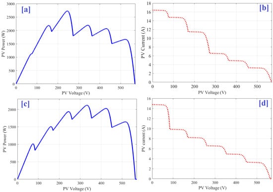
Figure 5.
The details of shadow patterns. (a) P-V curve first scenario, (b) I-V curve first scenario, (c) P-V curve second scenario, and (d) I–V curve second scenario.
Table 5.
Specification of shadow patterns and data at MPP.
To allow a fair comparison, both the number of populations (5) and iterations (20) were kept constants for all methods considered. During the optimization process, the product of PV current and (1 − D) was used as the objective function to be maximized. The decision variable is the duty cycle of DC-DC. To prove the consistency of the proposed mAHA, the studied algorithms were executed 30 times. The statistical analysis of the considered algorithms is shown in Table 6. The details of the 30 runs for both shadow scenarios are shown in Table 7.
Table 6.
Statistical assessments of considered algorithms for both shadow scenarios.
Table 7.
Cost function values during optimization process.
The two shadow scenarios are shown in Table 7, where the proposed mAHA has the best performance compared to other algorithms. For the first scenario, the average PV power values varied between 2716.754 W and 2067.039 W. mAHA achieves the maximum PV power of 2716.754 W, which is matched by HHO (2186.705 W). The minimum PV power of 2067.039 W is achieved by AHA. Thus, the proposed mAHA increases the PV power by 31.3% compared to the original AHA. The values of STD vary from 0.004308 to 0.516302. The minimum STD of 0.004308 is achieved by mAHA, followed by SMA (0.246108). The worst value of STD of 0.516302 is achieved by AHA. For the second shadow scenario, the average PV power values vary from 2119.219 W to 2094.641 W. mAHA achieves the maximum PV power of 2119.219 W, followed by WOA (2113.31 W). The minimum PV power of 2094.641 W is achieved by SMA. The values of STD vary from 0.000996 to 0.08421. The minimum STD of 0.000996 is achieved by mAHA, followed by HHO (0.047632). The worst value of STD of 0.08421 is obtained by SMA.
The mean cost function variation during optimization process for first and second shadow scenarios are presented in Figure 6 and Figure 7 respectively.
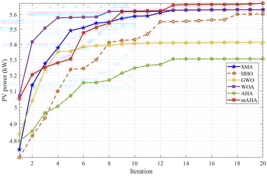
Figure 6.
Mean cost function variation during optimization process for first shadow scenario.
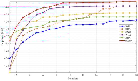
Figure 7.
Mean cost function variation during optimization process for second shadow scenario.
Table 8 shows the results of the analysis of variance (ANOVA), and Figure 8 shows the corresponding ranking. If the value of F is greater than the p value, the null hypothesis is true. The data collected show that the p-value is much lower than the F-value, indicating a significant difference between the results. As shown in Figure 8, the mAHA can outperform the other commonly used methods. The mAHA has the smallest range of variance and the largest mean fitness (maximization problem), indicating its resilience and accuracy.
Table 8.
ANOVA results for first shadow scenario.
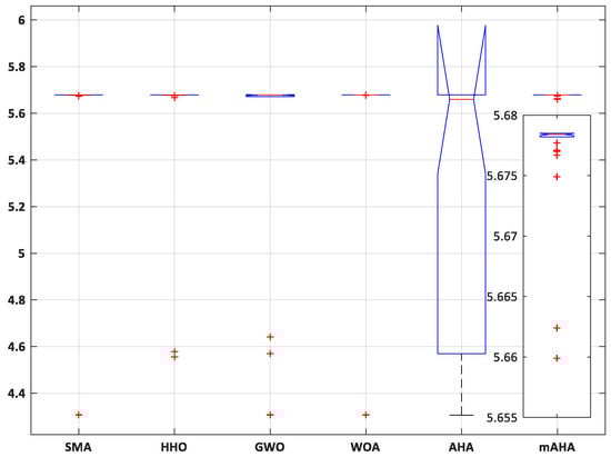
Figure 8.
ANOVA ranking for first shadow scenario.
A Tukey Honestly Significant Difference (Tukey HSD) post hoc analysis was performed to support the ANOVA results. The findings are shown in Figure 9. The mAHA has the greatest mean fitness. After the mAHA, the WAO and SMA provided good results.
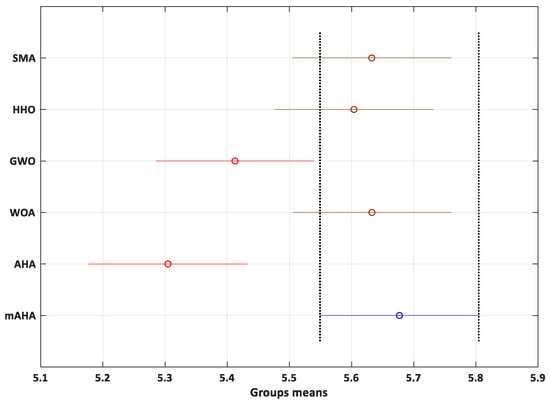
Figure 9.
Tukey test for first shadow scenario.
Table 9 shows the ANOVA test results for the second case, and Figure 10 shows the corresponding ranking. The obtained results show that the p-value is smaller than the F value, indicating a significant difference between the outcomes. As shown in Figure 10, the mAHA may outperform the other commonly used method. The mAHA has the smallest variance range and the greatest mean fitness (maximization problem), indicating its resilience and accuracy.
Table 9.
ANOVA results for the second shadow scenario.
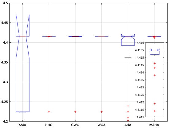
Figure 10.
ANOVA ranking for the second shadow scenario.
To support the ANOVA results for this case, a Tukey Honestly Significant Difference (Tukey HSD) post hoc analysis was performed. The findings are shown in Figure 11. Like the previous case, the mAHA has the greatest mean fitness. After the mAHA, the WAO and HHO provided good results.
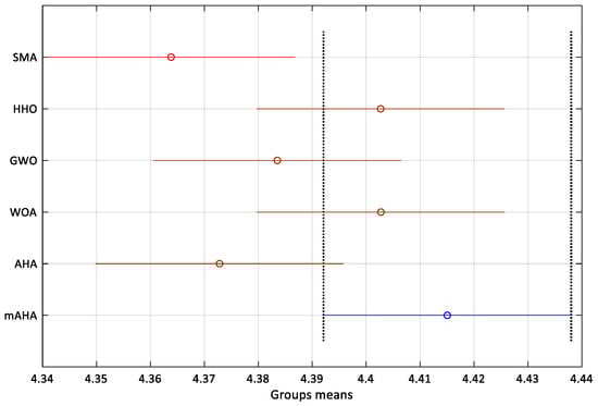
Figure 11.
Tukey test for the second shadow scenario.
6. Discussion
The aim of this study is to propose an effective optimization method for solving the optimization problem and finding the global maximum power point (MPP). In many occurrences, the proposed mAHA method achieved better or similar results.
The proposed mAHA method provides the following merits:
- The proposed mAHA was used for the first time to find the global maximum power point (MPP), includes 36 photovoltaic panels forming 6 arrays, DC-DC converter, controller, and 480 V battery bank.
- Table 6 shows the results of the analysis of variance (ANOVA), and Figure 8 shows the corresponding ranking. As shown in Figure 8, Figure 9, Figure 10 and Figure 11, the mAHA can outperform the other commonly used methods. The mAHA has the smallest range of variance and the largest mean fitness (maximization problem), indicating its resilience and accuracy.
- The obtained results show the superiority of the proposed single sensor-based MPPT method for PV systems. The scalability analysis demonstrated the robustness and flexibility of the proposed mAHA method.
Along with advantages, the proposed mAHA also has some limitations, which are detailed below:
- Despite eminent applications, AHA is still attributed for its slow convergence and stagnancy issues when employed on high-dimensional problems.
- The obtained solutions generated by mAHA may change each time it is run because it is an optimization strategy based on randomization. As a result, there is no assurance that the features subset chosen in one run will be present in another.
- The performance of the proposed mAHA method on complex and high dimensional problems may be worse according to the several mutations.
7. Conclusions
A modified version of the artificial hummingbird algorithm (AHA) has been proposed in this paper. It introduces the mechanisms of genetic operators (crossover and mutation selection) to enhance AHA’s performance in increasing the diversity of the population and avoiding local searches. After demonstration the superiority of mAHA, it has been used for first time to mitigate the shadow condition and extracting the global maximum power point (MPP) for photovoltaic (PV) system. The proposed MPP tracking (MPPT) technique needs only a single current sensor. Therefore, the cost of the controller will be reduced. Two shadow scenarios are used to evaluate the proposed single-sensor MPPT technique. For the first scenario, the average PV power values fluctuated between 2716.754 W and 2067.039 W. mAHA achieves the maximum PV power of 2716.754 W flowed by HHO (2186.705 W). The minimum PV power of 2067.039 W is obtained by AHA. Therefore, the proposed mAHA increased the PV power by 31.3% compared to the original AHA. For the second shadow scenario, the average PV power values fluctuated between 2119.219 W and 2094.641 W. mAHA achieves the maximum PV power of 2119.219 W flowed by WOA (2113.31W). The minimum PV power of 2094.641 W is obtained by SMA. The STD values varied between 0.000996 and 0.08421. According to the excellent efficiency obtained, the proposed mAHA can be applied in several real-world applications, such as object tracking, calculating solar cell parameters, electrical applications, hyperparameter optimization, and image segmentation.
Author Contributions
Conceptualization, E.H.H., H.R. and I.A.M.; Methodology, E.H.H. and H.R.; Software, E.H.H. and H.R.; Validation, I.A.M. and S.A.-S.; Formal analysis, H.A., E.H.H., H.R. and S.A.-S.; Investigation, H.R. and S.A.-S.; Resources, H.A., I.A.M. and S.A.-S.; Data curation, H.A. and I.A.M.; Writing—original draft, H.A., E.H.H., H.R., I.A.M. and S.A.-S.; Writing—review & editing, H.A., E.H.H., H.R., I.A.M. and S.A.-S.; Visualization, E.H.H. and H.R.; Supervision, E.H.H. and H.R.; Project administration, H.A.; Funding acquisition, H.A. All authors have read and agreed to the published version of the manuscript.
Funding
This research work was funded by the Deputyship for Research & Innovation, Ministry of Education in Saudi Arabia through the project number (IFPRC-78-135-2020) and King Abdulaziz University, DSR, Jeddah, Saudi Arabia.
Institutional Review Board Statement
Not applicable.
Informed Consent Statement
Not applicable.
Data Availability Statement
Not applicable.
Acknowledgments
The authors extend their appreciation to the Deputyship for Research & Innovation, Ministry of Education in Saudi Arabia for funding this research work through the project number (IFPRC-78-135-2020) and King Abdulaziz University, DSR, Jeddah, Saudi Arabia.
Conflicts of Interest
The authors declare no conflict of interest.
References
- Houssein, E.H.; Mahdy, M.A.; Shebl, D.; Manzoor, A.; Sarkar, R.; Mohamed, W.M. An efficient slime mould algorithm for solving multi-objective optimization problems. Expert Syst. Appl. 2022, 187, 115870. [Google Scholar] [CrossRef]
- Singh, N.; Houssein, E.H.; Singh, S.; Dhiman, G. Hssahho: A novel hybrid salp swarm-harris hawks optimization algorithm for complex engineering problems. J. Ambient. Intell. Humaniz. Comput. 2022, 97, 1–37. [Google Scholar]
- Houssein, E.H.; Gad, A.G.; Wazery, Y.M.; Suganthan, P.N. Task scheduling in cloud computing based on meta-heuristics: Review, taxonomy, open challenges, and future trends. Swarm Evol. Comput. 2021, 62, 100841. [Google Scholar] [CrossRef]
- Houssein, E.H.; Mahdy, M.A.; Blondin, M.J.; Shebl, D.; Mohamed, W.M. Hybrid slime mould algorithm with adaptive guided differential evolution algorithm for combinatorial and global optimization problems. Expert Syst. Appl. 2021, 174, 114689. [Google Scholar] [CrossRef]
- Houssein, E.H.; Mahdy, M.A.; Fathy, A.; Rezk, H. A modified Marine Predator Algorithm based on opposition based learning for tracking the global MPP of shaded PV system. Expert Syst. Appl. 2021, 183, 115253. [Google Scholar] [CrossRef]
- Lu, S.; Wang, C.; Fan, Y.; Lin, B. Robustness of building energy optimization with uncertainties using deterministic and stochastic methods: Analysis of two forms. Build. Environ. 2021, 205, 108185. [Google Scholar] [CrossRef]
- Forrest, S. Genetic algorithms. ACM Comput. Surv. 1996, 28, 77–80. [Google Scholar] [CrossRef]
- Eberhart, R.; Kennedy, J. Particle swarm optimization. In Proceedings of the IEEE International Conference on Neural Networks, Perth, Australia, 27 November–1 December 1995; Volume 4, pp. 1942–1948. [Google Scholar]
- Teodorović, D. Bee colony optimization (BCO). In Innovations in Swarm Intelligence; Springer: Berlin/Heidelberg, Germany, 2009; pp. 39–60. [Google Scholar]
- Storn, R.; Kenneth, P. Differential evolution–a simple and efficient heuristic for global optimization over continuous spaces. J. Glob. Optim. 1997, 11, 341–359. [Google Scholar] [CrossRef]
- Houssein, E.H.; Abdelkareem, D.A.; Emam, M.M.; Hameed, M.A.; Younan, M. An efficient image segmentation method for skin cancer imaging using improved golden jackal optimization algorithm. Comput. Biol. Med. 2022, 149, 106075. [Google Scholar] [CrossRef]
- Houssein, E.H.; Emam, M.M.; Ali, A.A.; Suganthan, P.N. Deep and machine learning techniques for medical imaging-based breast cancer: A comprehensive review. Expert Syst. Appl. 2021, 167, 114161. [Google Scholar] [CrossRef]
- Houssein, E.H.; Emam, M.M.; Ali, A.A. Improved manta ray foraging optimization for multi-level thresholding using COVID-19 CT images. Neural Comput. Appl. 2021, 33, 16899–16919. [Google Scholar] [CrossRef] [PubMed]
- Houssein, E.H.; Abohashima, Z.; Elhoseny, M.; Mohamed, W.M. Hybrid quantum-classical convolutional neural network model for COVID-19 prediction using chest X-ray images. J. Comput. Des. Eng. 2022, 9, 343–363. [Google Scholar] [CrossRef]
- Houssein, E.H.; Oliva, D.; Çelik, E.; Emam, M.M.; Ghoniem, R.M. Boosted sooty tern optimization algorithm for global optimization and feature selection. Expert Syst. Appl. 2023, 213, 119015. [Google Scholar] [CrossRef]
- Houssein, E.H.; Hosney, M.E.; Mohamed, W.M.; Ali, A.A.; Younis, E.M. Fuzzy-based hunger games search algorithm for global optimization and feature selection using medical data. Neural Comput. Appl. 2022, 1–25. [Google Scholar] [CrossRef] [PubMed]
- Emam, M.M.; Houssein, E.H.; Ghoniem, R.M. A modified reptile search algorithm for global optimization and image segmentation: Case study brain MRI images. Comput. Biol. Med. 2023, 152, 106404. [Google Scholar] [CrossRef] [PubMed]
- Hashim, F.A.; Hussain, K.; Houssein, E.H.; Mabrouk, M.S.; Al-Atabany, W. Archimedes optimization algorithm: A new metaheuristic algorithm for solving optimization problems. Appl. Intell. 2021, 51, 1531–1551. [Google Scholar] [CrossRef]
- Houssein, E.H.; Çelik, E.; Mahdy, M.A.; Ghoniem, R.M. Self-adaptive Equilibrium Optimizer for solving global, combinatorial, engineering, and Multi-Objective problems. Expert Syst. Appl. 2022, 195, 116552. [Google Scholar] [CrossRef]
- Houssein, E.H.; Saad, M.R.; Hashim, F.A.; Shaban, H.; Hassaballah, M. Lévy flight distribution: A new metaheuristic algorithm for solving engineering optimization problems. Eng. Appl. Artif. Intell. 2020, 94, 103731. [Google Scholar] [CrossRef]
- Zhao, W.; Wang, L.; Mirjalili, S. Artificial hummingbird algorithm: A new bio-inspired optimizer with its engineering applications. Comput. Methods Appl. Mech. Eng. 2022, 388, 114194. [Google Scholar] [CrossRef]
- Li, S.; Chen, H.; Wang, M.; Heidari, A.A.; Mirjalili, S. Slime mould algorithm: A new method for stochastic optimization. Future Gener. Comput. Syst. 2020, 111, 300–323. [Google Scholar] [CrossRef]
- Heidari, A.A.; Mirjalili, S.; Faris, H.; Aljarah, I.; Mafarja, M.; Chen, H. Harris hawks optimization: Algorithm and applications. Future Gener. Comput. Syst. 2019, 97, 849–872. [Google Scholar] [CrossRef]
- Mirjalili, S.; Mirjalili, S.M.; Lewis, A. Grey wolf optimizer. Adv. Eng. Softw. 2014, 69, 46–61. [Google Scholar] [CrossRef]
- Mirjalili, S.; Andrew, L. The whale optimization algorithm. Adv. Eng. Softw. 2016, 95, 51–67. [Google Scholar] [CrossRef]
- Krupnov, Y.A.; Krasilnikova, V.G.; Kiselev, V.; Yashchenko, A.V. The Contribution of Sustainable and Clean Energy to the Strengthening of Energy Security. Front. Environ. Sci. 2022, 10, 2505. [Google Scholar] [CrossRef]
- Zsiborács, H.; Pintér, G.; Vincze, A.; Baranyai, N.H.; Mayer, M.J. The reliability of photovoltaic power generation scheduling in seventeen European countries. Energy Convers. Manag. 2022, 260, 115641. [Google Scholar] [CrossRef]
- Karmouni, H.; Chouiekh, M.; Motahhir, S.; Qjidaa, H.; Jamil, M.O.; Sayyouri, M. A fast and accurate sine-cosine MPPT algorithm under partial shading with implementation using arduino board. Clean. Eng. Technol. 2022, 9, 100535. [Google Scholar] [CrossRef]
- Bhukya, L.; Kedika, N.R.; Salkuti, S.R. Enhanced Maximum Power Point Techniques for Solar Photovoltaic System under Uniform Insolation and Partial Shading Conditions: A Review. Algorithms 2022, 15, 365. [Google Scholar] [CrossRef]
- Boghdady, T.A.; Kotb, Y.E.; Aljumah, A.; Sayed, M.M. Comparative Study of Optimal PV Array Configurations and MPPT under Partial Shading with Fast Dynamical Change of Hybrid Load. Sustainability 2022, 14, 2937. [Google Scholar] [CrossRef]
- Zafar, M.H.; Khan, N.M.; Mirza, A.F.; Mansoor, M. Bio-inspired optimization algorithms based maximum power point tracking technique for photovoltaic systems under partial shading and complex partial shading conditions. J. Clean. Prod. 2021, 309, 127279. [Google Scholar] [CrossRef]
- Zafar, M.H.; Khan, N.M.; Mirza, A.F.; Mansoor, M.; Akhtar, N.; Qadir, M.U.; Khan, N.A.; Moosavi, S.K.R. A novel meta-heuristic optimization algorithm based MPPT control technique for PV systems under complex partial shading condition. Sustain. Energy Technol. Assess. 2021, 47, 101367. [Google Scholar]
- Zafar, M.H.; Al-shahrani, T.; Khan, N.M.; Mirza, A.F.; Mansoor, M.; Qadir, M.U.; Khan, M.I.; Naqvi, R.A. Group teaching optimization algorithm based MPPT control of PV systems under partial shading and complex partial shading. Electronics 2020, 9, 1962. [Google Scholar] [CrossRef]
- Huang, Y.-P.; Chen, X.; Ye, C.-E. A hybrid maximum power point tracking approach for photovoltaic systems under partial shading conditions using a modified genetic algorithm and the firefly algorithm. Int. J. Photoenergy 2018, 7598653. [Google Scholar] [CrossRef]
- El-Helw, H.M.; Magdy, A.; Marei, M.I. A Hybrid Maximum Power Point Tracking Technique for Partially Shaded Photovoltaic Arrays. IEEE Access 2017, 5, 11900–11908. [Google Scholar] [CrossRef]
- El-Shafy, K.A.; Nafeh, A. An effective and safe charging algorithm for lead-acid batteries in PV systems. Int. J. Energy Res. 2011, 35, 733–740. [Google Scholar]
- Camilo, J.C.; Guedes, T.; Fernandes, D.A.; Melo, J.; Costa, F.; Filho, A.J.S. A maximum power point tracking for photovoltaic systems based on Monod equation. Renew. Energy 2019, 130, 428–438. [Google Scholar] [CrossRef]
- Zhou, Y.; Wang, Y.; Wang, K.; Kang, L.; Peng, F.; Wang, L.; Pang, J. Hybrid genetic algorithm method for efficient and robust evaluation of remaining useful life of supercapacitors. Appl. Energy 2020, 260, 114169. [Google Scholar] [CrossRef]
- Mohamed, A.W.; Hadi, A.A.; Mohamed, A.K.; Awad, N.H. Evaluating the performance of adaptive gaining sharing knowledge based algorithm on CEC 2020 benchmark problems. In Proceedings of the 2020 IEEE Congress on Evolutionary Computation (CEC), Glasgow, UK, 19–24 July 2020; IEEE: Piscataway, NJ, USA, 2020; pp. 1–8. [Google Scholar]
- Biswas; Subhodip; Saha, D.; De, S.; Cobb, A.D.; Das, S.; Jalaian, B.A. Improving differential evolution through Bayesian hyperparameter optimization. In Proceedings of the 2021 IEEE Congress on Evolutionary Computation (CEC), Kraków, Poland, 28 June–1 July 2021; IEEE: Piscataway, NJ, USA, 2021; pp. 832–840. [Google Scholar]
- Saha, D.; Sallam, K.M.; De, S.; Mohamed, A.W. Framework of Ensemble Parmeter Adapted Evolutionary Algorithm for Solving Constrained Optimization Problems. Preprints 2022. [Google Scholar] [CrossRef]
- Mohamed, A.W.; Hadi, A.A.; Agrawal, P.; Sallam, K.M.; Mohamed, A.K. Gaining-sharing knowledge based algorithm with adaptive parameters hybrid with imode algorithm for solving cec 2021 benchmark problems. In Proceedings of the 2021 IEEE Congress on Evolutionary Computation (CEC), Kraków, Poland, 28 June–1 July 2021; IEEE: Piscataway, NJ, USA, 2021; pp. 841–848. [Google Scholar]
- Houssein, E.H.; Rezk, H.; Fathy, A.; Mahdy, M.A.; Nassef, A.M. A modified adaptive guided differential evolution algorithm applied to engineering applications. Eng. Appl. Artif. Intell. 2022, 113, 104920. [Google Scholar] [CrossRef]


Disclaimer/Publisher’s Note: The statements, opinions and data contained in all publications are solely those of the individual author(s) and contributor(s) and not of MDPI and/or the editor(s). MDPI and/or the editor(s) disclaim responsibility for any injury to people or property resulting from any ideas, methods, instructions or products referred to in the content. |
© 2023 by the authors. Licensee MDPI, Basel, Switzerland. This article is an open access article distributed under the terms and conditions of the Creative Commons Attribution (CC BY) license (https://creativecommons.org/licenses/by/4.0/).