The Exponentiated Power Alpha Index Generalized Family of Distributions: Properties and Applications

Abstract

The study of hydrological characteristics has a vital role in designing, planning, and managing water resources. The selection of appropriate probability distributions and methods of estimations are basic elements in hydrology analyses. In this article, a new family named the ‘exponentiated power alpha index generalized’ (EPAIG)-G is proposed to develop several new distributions. Using this proposed family, we developed a new model, called the EPAIG-exponential (EPAIG-E). A few structural properties of the EPAIG-G were obtained. The EPAIG-E parameters were estimated through the method of maximum likelihood (MML). The study of the Monte Carlo simulation (MCS) was produced for the EPAIG-E. The model performance is illustrated using real data.

1. Introduction

In a variety of fields, the exponential distribution (ED) is commonly used for the examination of data. ED, at times, performs well with different datasets; however, in several practical instances, it is not flexible enough to examine the complicated behaviors shown by the data. Therefore, the consideration involves more flexible distributions, which can fit any type of data with any level of intricacy. To put a new parameter to the baseline distribution (BLD), Gupta et al. (1998) [1] proposed the exponentiated method (EM) with the parameter being the power of the cumulative distribution function (cdf), which provides adaptable and more flexible distributions. Let the cdf $F(\xi ;x)$ be the continuous BLD with a random variable (r.v.) X, then the exponentiated derived distribution cdf is

$$G_{EM}(\xi ,\beta ;x)={\left[F(\xi ;x)\right]}^{\beta };x>0,\beta >0.$$

(1)

where $\beta$ is an extra shape/power parameter and $\xi$ is the BLD parameter.

Recently, to obtain a more flexible family of distributions (FoDs), Mahdavi and Kundu (2017) [2] proposed the alpha power method (APM). The cdf of the APM family with continuous r.v. X is defined as

$$G_{APM}(\xi ,\alpha ;x)=\frac{{\alpha }^{F(\xi ;x)}-1}{\alpha -1};\alpha \ne 1,\alpha ,x>0.$$

(2)

Many researchers have applied the EM and APM on different traditional distributions. Gupta and Kundu (2001) [3] derived the generalized exponential (GE) (also called the exponentiated exponential (EE)) distribution with two parameters—the shape ($\beta >0$) and scale ($\theta >0$). The cdf of the EE distribution (EED) is defined as

$$G_{EE}(\beta ,\theta ;x)={(1-e^{-\theta x})}^{\beta };x>0.$$

(3)

The probability density function (pdf) of EED varies significantly based on $\beta$. Moreover, if $\beta <1$, the hazard function (HF) of EED is a non-increasing function, and if $\beta >1$, it is a non-decreasing function. The HF is constant when $\beta =1$. Clearly, the ED is a special case of EED for $\beta =1$. Naturally, EE and gamma distributions have several properties that are quite similar, but EED has explicit expressions and the reliability functions (RFs) are identical to the Weibull distribution. In different manners, the EE, Weibull, and gamma distributions extend the ED. For more details on EMs and the exponentiated family of distributions, we refer to Tahir and Nadarajah (2015) [4], ElSherpieny and Almetwally (2022) [5], and Hussain et al. (2022) [6].

Developing new FoDs is another forceful method to derive more flexible distributions. For any continuous distribution (CD), generators of various types can be practiced to obtain new FoDs. Alzaatreh et al. (2013) [7] derived the transformed-transformer method (also called the T-X family) for generating new FoDs as any CD considered a generator. Let X be a r.v. for any CD, then the family T-X cdf is

$$G_{TX}(\xi ;x)={\int }_{v_1}^{W\left[F\right(\xi ;x\left)\right]}r\left(t\right)\mathrm{d}t.$$

(4)

where under the control of $\xi$, $F(\xi ;x)$ is the cdf of any BLD, $W\left[F(\xi ;x)\right]\in [v_1,v_2]$ at that $x\in [-\infty ,\infty ]$ is a monotone increasing–differentiable function of $F(\xi ;x)$, and $r\left(t\right)$ is the pdf of r.v. $T\in [v_1,v_2]$ as $-\infty <v_1<v_2<\infty$. A new class of FoDs will be obtained using different transformers $W\left[F\right(\xi ;x\left)\right]$.

In view of the EM Equation (1), the APM Equation (2), and the T-X family Equation (4), we developed a new class by the name of the exponentiated power alpha index generalized-G (EPAIG-G) family. Let cdf

$$R\left(t\right)={\left(\frac{{\alpha }^t-1}{\alpha -1}\right)}^{\beta };t\ge 0,$$

(5)

of r.v. T. The pdf conforming to Equation (5) is

$$r\left(t\right)=\frac{\beta }{\alpha -1}log\alpha {\left(\frac{{\alpha }^t-1}{\alpha -1}\right)}^{\beta -1}{\alpha }^t,t>0.$$

(6)

Here, we use

$$W\left[F(\xi ;x)\right]=\frac{H(\xi ;x)}{H(\xi ;x)+1}.$$

(7)

as the transformer, and $H(\xi ;x)=-log[1-F(\xi ;x\left)\right]$ is the cumulative hazard rate function (CHRF) of BLD. Setting Equations (7) and (6) in Equation (4), then the cdf of the EPAIG-G family is defined as

$$\begin{array}{cc}\hfill G_{EPAIG}(\xi ,\beta ,\alpha ;x)& =\frac{\beta log\alpha }{\alpha -1}{\int }_0^{\frac{H(\xi ;x)}{H(\xi ;x)+1}}{\left(\frac{{\alpha }^t-1}{\alpha -1}\right)}^{\beta -1}{\alpha }^t\mathrm{d}t,\hfill \\ \hfill & ={\left(\frac{{\alpha }^{\frac{H(\xi ;x)}{H(\xi ;x)+1}}-1}{\alpha -1}\right)}^{\beta }=R\left(\frac{H(\xi ;x)}{H(\xi ;x)+1}\right);\xi ,\alpha ,\beta ,x>0,\alpha \ne 1.\hfill \end{array}$$

(8)

The pdf of the EPAIG-G family corresponds to Equation (8), and is given as

$$\begin{array}{cc}\hfill g_{EPAIG}(\xi ,\beta ,\alpha ;x)& =\frac{\beta log\alpha }{\alpha -1}{\left(\frac{{\alpha }^{\frac{H(\xi ;x)}{H(\xi ;x)+1}}-1}{\alpha -1}\right)}^{\beta -1}{\alpha }^{\frac{H(\xi ;x)}{H(\xi ;x)+1}}\frac{h(\xi ;x)}{{[H(\xi ;x)+1]}^2},\hfill \\ \hfill & =r\left(\frac{H(\xi ;x)}{H(\xi ;x)+1}\right)\frac{h(\xi ;x)}{{[H(\xi ;x)+1]}^2}.\hfill \end{array}$$

(9)

where $h(\xi ;x)$ is the hazard rate function (HRF) of BLD.

The reliability measures of X follow EPAIG-G ($\xi ,\beta ,\alpha$) with pdf Equation (9) defined below.

i.

The RF of the EPAIG-G family, using Equation (8), is

$$R_{EPAIG}(\xi ,\beta ,\alpha ;x)=1-{\left({(\alpha -1)}^{-1}\left\{{\alpha }^{\frac{H(\xi ;x)}{H(\xi ;x)+1}}-1\right\}\right)}^{\beta }$$

ii.

The HRF, CHRF, and reversed HRF of the EPAIG-G family are defined below:

$$h_{EPAIG}(\xi ,\beta ,\alpha ;x)=\frac{\beta log\alpha {\left[1-{\alpha }^{-\frac{H(\xi ;x)}{H(\xi ;x)+1}}\right]}^{-1}{\left[H(\xi ;x)+1\right]}^{-2}h(\xi ;x)}{{\left[(\alpha -1){\left({\alpha }^{\frac{H(\xi ;x)}{H(\xi ;x)+1}}-1\right)}^{-1}\right]}^{\beta }-1}$$

$$H_{EPAIG}(\xi ,\beta ,\alpha ;x)=-log\left[1-{\left\{{(1-\alpha )}^{-1}\left(1-{\alpha }^{\frac{H(\xi ;x)}{H(\xi ;x)+1}}\right)\right\}}^{\beta }\right]$$

$$r_{EPAIG}(\xi ,\beta ,\alpha ;x)=\frac{\beta log\alpha h(\xi ;x)}{{\left[H(\xi ;x)+1\right]}^2\left[1-{\alpha }^{-\frac{H(\xi ;x)}{H(\xi ;x)+1}}\right]}$$

The article layout is as follows. In Section 1, a new family called EPAIG-G is introduced with its reliability measures. We obtained useful expansion and derived structural properties of the EPAIG-G, respectively, in Section 2 and Section 3. The estimations by MML of the parameters of the EPAIG-G family are presented in Section 4. Section 5 explains the proposed EPAIG-E model and its pdf and HRF plots. Inside this section, the MCS study was performed to assess the performance of the EPAIG-E model. The potentiality of the EPAIG-E is also illustrated through real data. Finally, Section 6 presents our conclusions.

2. Useful Expansions of the EPAIG-G Family

The expansion of binomial (EoB) is

$${\left(1-Z\right)}^{\beta }=\sum _{m=0}^{\infty }{(-1)}^m\left(\genfrac{}{}{0pt}{}{\beta }{m}\right)Z^m$$

(10)

Applying Equation (10) to Equation (8), we have

$$G_{EPAIG}(\xi ,\beta ,\alpha ;x)=\frac{1}{{\left(1-\alpha \right)}^{\beta }}\sum _{m=0}^{\infty }{(-1)}^m\left(\genfrac{}{}{0pt}{}{\beta }{m}\right){\alpha }^{m\frac{H(\xi ;x)}{H(\xi ;x)+1}}$$

(11)

The Maclaurin series for ${\alpha }^y$ is

$${\alpha }^y=\sum _{i=0}^{\infty }\frac{{(log\alpha )}^i{y}^i}{i!}$$

(12)

Using Equation (12) in Equation (11), we obtain

$$G_{EPAIG}(\xi ,\beta ,\alpha ;x)=\frac{1}{{(1-\alpha )}^{\beta }}\sum _{m=0}^{\infty }\sum _{i=0}^{\infty }\frac{{(-1)}^m}{i!}\left(\genfrac{}{}{0pt}{}{\beta }{m}\right){(log\alpha )}^i{m}^i{[H(\xi ;x)+1]}^{-i}{\left[H(\xi ;x)\right]}^i$$

(13)

The EoB series ${(1+Z)}^{-\beta }$ for the non-integer real positive $\beta$ and $\left|Z\right|<1$ is

$${\left(1+Z\right)}^{-\beta }=\sum _{j=0}^{\infty }{(-1)}^j\left(\genfrac{}{}{0pt}{}{\beta +j-1}{j}\right)Z^j$$

(14)

By inserting Equation (14) in Equation (13), we have

$$G_{EPAIG}(\xi ,\beta ,\alpha ;x)=\sum _{m=0}^{\infty }\sum _{i=0}^{\infty }\sum _{j=0}^{\infty }\frac{{(-1)}^{m+j}{m}^i{(log\alpha )}^i}{{(1-\alpha )}^{\beta }i!}\left(\genfrac{}{}{0pt}{}{\beta }{m}\right)\left(\genfrac{}{}{0pt}{}{\beta +j-1}{j}\right){\left[H(\xi ;x)\right]}^{i+j}$$

(15)

For the arbitrary parameters $A_1\in R$ and $A_2\in (0,1)$, it can be proven that

$${[-log(1-A_2)]}^{A_1}=A_2^{A_1}+A_1\sum _{k=0}^{\infty }{p}_k(A_1+k)A_2^{k+A_1+1}$$

(16)

where $p_k\left(A_1\right)$ are Stirling polynomials. For details of Equation (16), see Flajonet and Odlyzko (1990); Flajonet and Sedgewick (2009) [8,9]. Applying Equation (16), we obtain ${\left[H(\xi ;x)\right]}^{i+j}$ using $H(\xi ;x)=-log\left[1-F(\xi ;x)\right]$, which is equal to

$${\left[H(\xi ;x)\right]}^{i+j}={\left[F(\xi ;x)\right]}^{i+j}+(i+j)\sum _{k=0}^{\infty }{p}_k(i+j+k){\left[F(\xi ;x)\right]}^{k+(i+j)+1}$$

(17)

The power series $Z^{\beta }$ is

$$Z^{\beta }=\sum _{l_1=0}^{\infty }\sum _{l_2=l_1}^{\infty }{(-1)}^{l_2+l_1}\left(\genfrac{}{}{0pt}{}{\beta }{l_2}\right)\left(\genfrac{}{}{0pt}{}{l_2}{l_1}\right)Z^{l_1}$$

(18)

Expanding Equation (17) in Equation (18), we have

$${\left[H(\xi ;x)\right]}^{i+j}=\sum _{l_1=0}^{\infty }\left\{\sum _{l_2=0}^{\infty }{(-1)}^{l_2+l_1}\left(\genfrac{}{}{0pt}{}{l_2}{l_1}\right)\left[\left(\genfrac{}{}{0pt}{}{i+j}{l_2}\right)+(i+j)\sum _{k=0}^{\infty }{p}_k(i+j+k)\left(\genfrac{}{}{0pt}{}{k+(i+j)+1}{l_2}\right)\right]\right\}F{(\xi ;x)}^{l_1}$$

(19)

By substituting Equation (19) with Equation (15), we have

$$G_{EPAIG}(\xi ,\beta ,\alpha ;x)=\sum _{l_1=0}^{\infty }{W}_{l_1}F{(\xi ;x)}^{l_1}$$

(20)

where

$$\begin{array}{cc}\hfill W_{l_1}=& \sum _{m,i,j,l_2=0}^{\infty }{(-1)}^{m+j+l_1+l_2}\frac{{(log\alpha )}^i{m}^i}{{(1-\alpha )}^{\beta }i!}\left(\genfrac{}{}{0pt}{}{\beta }{m}\right)\left(\genfrac{}{}{0pt}{}{l_2}{l_1}\right)\left(\genfrac{}{}{0pt}{}{\beta +j-1}{j}\right)\times \hfill \\ \hfill & \left[\left(\genfrac{}{}{0pt}{}{i+j}{l_2}\right)+(i+j)\sum _{k=0}^{\infty }{p}_k(i+j+k)\left(\genfrac{}{}{0pt}{}{k+(i+j)+1}{l_2}\right)\right]\hfill \end{array}$$

(21)

Equation (20) was extracted as

$$G(\xi ,\beta ,\alpha ;x)=\sum _{l_1=0}^{\infty }{W}_{l_1}{H}_{l_1}(\xi ;x)$$

(22)

where $H_{l_1}(\xi ;x)=F{(\xi ;x)}^{l_1}$ presents the exponentiated-G (exp-G ($l_1$)) cdf.

The pdf of X corresponding to Equation (20), using Equations (10), (12), (14), (16) and (18) in Equation (9), respectively, can be defined as

$$g_{EPAIG}(\xi ,\beta ,\alpha ;x)=\sum _{l_1=0}^{\infty }{\eta }_{l_1}F{(\xi ;x)}^{l_1}f(\xi ;x)$$

(23)

where

$$\begin{array}{cc}\hfill {\eta }_{l_1}=& \sum _{l_2,m,k,i,j=0}^{\infty }\frac{\beta {(1+i)}^j{(log\alpha )}^{1+j}}{j!{(\alpha -1)}^{\beta }}\left(\genfrac{}{}{0pt}{}{\beta -1}{i}\right)\left(\genfrac{}{}{0pt}{}{(2+j)+k-1}{k}\right){(-1)}^{\beta +i+k+l_1+l_2-1}\hfill \\ \hfill & \times \left(\genfrac{}{}{0pt}{}{l_2}{l_1}\right)\left[\left(\genfrac{}{}{0pt}{}{m+k+j}{l_2}\right)+(j+k)\sum _{s=0}^{\infty }{p}_s(k+j+s)\left(\genfrac{}{}{0pt}{}{m+s+1+(k+j)}{l_2}\right)\right]\hfill \end{array}$$

From Equation (23), another extracted form of the pdf with the infinite linear combination is given as

$$g(\xi ,\beta ,\alpha ;x)=\sum _{l_1=0}^{\infty }{w}_{l_1}{h}_{(l_1+1)}(\xi ;x)$$

(24)

where $w_{l_1}=\frac{{\eta }_{l_1}}{l_1+1}$, $h_{(l_1+1)}(\xi ;x)=(l_1+1)F{(\xi ;x)}^{l_1}f(\xi ;x)$ is the density of exp-G, with $l_1+1$ as the power parameter.

3. Structural Properties of the EPAIG-G Family

The properties of the EPAIG-G structure from Equation (24) and of exp-G properties can be derived as follows.

3.1. Quantile Function (QF)

Let $Q_F(\xi ;u)=F^{-1}(\xi ;u)$; $0<u<1$ be the QF of BLD. Inverting $G_{EPAIG}(\xi ,\beta ,\alpha ;x)=u$ in Equation (8), we obtain the QF of X as

$$x=G^{-1}(\xi ,\beta ,\alpha ;u)=Q_F\left(1-exp\left\{{\left[1-log\alpha {\left\{log\left(1+(\alpha -1)u^{\frac{1}{\beta }}\right)\right\}}^{-1}\right]}^{-1}\right\}\right)$$

(25)

Equation (25) reveals the QF of the EPAIG-G, which is based on the BLD QF. By substituting suitable u values in Equation (25), quantiles of interest can be obtained. In particular, when $u=0.5$, the median of X is expressed as

$$x_{0.5}=Q_F\left(1-exp\left\{{\left[1-log\alpha {\left\{log\left(1+(\alpha -1){\left(0.5\right)}^{\frac{1}{\beta }}\right)\right\}}^{-1}\right]}^{-1}\right\}\right)$$

Equation (25) can also be used for simulating EPAIG-G r.v.’s using the uniform r.v. $u\in (0,1)$.

3.2. Moments

Let a r.v. $Z_{l_1+1}$ follow exp-G ($l_1+1$) with pdf $h_{(l_1+1)}(\xi ;x)$. The nth ordinary moments (OMs) of X follow Equation (24), and can be obtained as

$${\mu }_n^{\prime }=E\left(X^n\right)=\sum _{l_1=0}^{\infty }{w}_{l_1}E\left(Z_{l_1+1}^n\right)$$

(26)

Another formula for ${\mu }_n^{\prime }$ from Equation (24) can be acquired in the BLD QF $Q_F(\xi ;u)$ reference. We have

$${\mu }_n^{\prime }=\sum _{l_1=0}^{\infty }(l_1+1)w_{l_1}\tau (n,l_1)$$

(27)

where $\tau (n,l_1)$, in connection with F QF, is

$$\tau (n,l_1)={\int }_{-\infty }^{\infty }{x}^{n}F{(\xi ;x)}^{l_1}f(\xi ;x)\mathrm{d}x={\int }_0^1{Q}_F{(\xi ;u)}^n{u}^{l_1}\mathrm{d}u$$

In addition, for X, the mean moments ${\mu }_n$ and cumulants ${\kappa }_n$ for Equation (24) can be obtained as

$${\mu }_n=\sum _{l_1=0}^n{(-1)}^{l_1}\left(\genfrac{}{}{0pt}{}{n}{l_1}\right){\left({\mu }_1^{\prime }\right)}^{l_1}{\mu }_{n-l_1}^{\prime }$$

(28)

and

$${\kappa }_n={\mu }_n^{\prime }-\sum _{l_1=1}^{n-1}\left(\genfrac{}{}{0pt}{}{n-1}{l_1-1}\right){\kappa }_{l_1}{\mu }_{n-l_1}^{\prime }$$

(29)

respectively, where ${\kappa }_1={\mu }_1^{\prime }$.

By the nth incomplete moment (IM) of X, using Equation (24), we can write

$$m_n\left(z\right)=\sum _{l_1=0}^{\infty }(l_1+1)w_{l_1}{T}_{n,l_1}\left(z\right)$$

(30)

where $T_{n,l_1}\left(z\right)$ can be computed for the F BLD.

$$\begin{array}{cc}\hfill T_{n,l_1}\left(z\right)& ={\int }_{-\infty }^z{x}^{n}F{(\xi ;x)}^{l_1}f(\xi ;x)\mathrm{d}x\hfill \\ & ={\int }_0^{F\left(z\right)}{Q}_F{(\xi ;u)}^n{u}^{l_1}\mathrm{d}u\hfill \end{array}$$

Setting $n=1$ in Equation (30) gives the first IM. The first IM of X is important to obtain the mean deviations, which can be applied to measure the dispersion amount in a population, and the curves of Lorenz and Bonferroni, which have appropriate empirical applications in areas of reliability, economics, demography, and many others.

The nth factorial descending moment (FDM) of X is evaluated as:

$$\begin{array}{cc}\hfill {\mu }_{\left(n\right)}^{\prime }=E\left[X^{\left(n\right)}\right]=& E\left[\prod _{a=0}^{n-1}(X-a)\right]\hfill \\ \hfill & =\sum _{l_1=0}^{n}s(n,l_1){\mu }_{l_1}^{\prime }\hfill \end{array}$$

(31)

where

$$s(n,l_1)=\frac{1}{l_1!}{\left[\frac{{\mathrm{d}}^{l_1}}{\mathrm{d}{x}^{l_1}}{x}^{\left(n\right)}\right]}_{x=0}$$

is the Stirling number of the first kind that permutes the n-item list into cycles $l_1$.

3.3. Moment Generating Function (MGF)

Here, we provide the MGF of X, i.e., $M_X\left(t\right)=E[exp\left(tx\right)]$. From Equation (24):

$$M_X\left(t\right)=\sum _{l_1=0}^{\infty }{w}_{l_1}{M}_{l_1+1}\left(t\right)$$

(32)

where $M_{l_1+1}\left(t\right)$ is the MGF of $Z_{l_1+1}$. Because of that, $M_X\left(t\right)$ can come by the MGF of exp-G($l_1+1$).

Alternatively, $M_X\left(t\right)$ can be expressed from Equation (24) as

$$M_X\left(t\right)=\sum _{l_1=0}^{\infty }(l_1+1)w_{l_1}\rho (t,l_1)$$

(33)

where

$$\rho (t,l_1)={\int }_{-\infty }^{\infty }exp\left(tx\right)F{(\xi ;x)}^{l_1}f(\xi ;x)\mathrm{d}x={\int }_0^{1}exp\left[t{Q}_F(\xi ;u)\right]u^{l_1}\mathrm{d}u$$

3.4. Mean Deviations (MDs)

The formulae are given below:

$${\delta }_{\mu }=E\left(\right|X-\mu \left|\right)={\int }_{-\infty }^{\infty }|x-\mu |g(\xi ,\beta ,\alpha ;x)\mathrm{d}x$$

(34)

and

$${\delta }_M=E\left(\right|X-M\left|\right)={\int }_{-\infty }^{\infty }|x-M|g(\xi ,\beta ,\alpha ;x)\mathrm{d}x$$

(35)

describe the MDs of X through the mean $\mu ={\mu }_1^{\prime }$ and over the median M, respectively, $g(\xi ,\beta ,\alpha ;x)$ is the pdf from Equation (24). Using Equation (30) by setting $n=1$, the formulae in Equations (34) and (35) can be expressed as

$${\delta }_{\mu }\left(X\right)=-2[m_1\left(\mu \right)-\mu G\left(\mu \right)]$$

(36)

and

$${\delta }_M\left(X\right)=-2[m_1\left(M\right)-\frac{\mu }{2}]$$

(37)

where $G\left(\mu \right)$ is the cdf from Equation (8) evaluated at $\mu$ and the first IM from Equation (24) is given below

$$m_1\left(z\right)=\sum _{l_1=0}^{\infty }(l_1+1)w_{l_1}{T}_{1,l_1}\left(z\right)$$

(38)

where

$$T_{1,l_1}\left(z\right)={\int }_{-\infty }^{z}xF{(\xi ;x)}^{l_1}f(\xi ;x)\mathrm{d}x={\int }_0^{F\left(z\right)}{Q}_F(\xi ;u)u^{l_1}\mathrm{d}u$$

(39)

Equation (39) is the fundamental quantity used to determine MDs of exp-G ($l_1+1$) distributions. Therefore, MDs inside Equations (36) and (37) depend only on MDs of distribution of exp-G.

3.5. Lorenz and Bonferroni Curves

For a specified probability $\pi$, and using the first IM given in Equation (38), the Lorenz and Bonferroni curves of X are described as

$$L\left(\pi \right)=\frac{1}{\mu {\left[m_1\left(q\right)\right]}^{-1}}$$

(40)

and

$$B\left(\pi \right)={\left(\pi \mu \right)}^{-1}\left[m_1\left(q\right)\right]$$

(41)

where $\mu ={\mu }_1^{\prime }$ and $q=Q_G(\xi ,\beta ,\alpha ;\pi )$ is determined by Equation (25).

3.6. Probability Weighted Moments (PWMs)

For r.v. X, the $(n,s)$th PWMs are given as

$$\begin{array}{cc}\hfill {\kappa }_{n,s}& =E\left[X^{n}G{(\xi ,\beta ,\alpha ;x)}^s\right]\hfill \\ \hfill & ={\int }_{-\infty }^{\infty }{x}^{n}G{(\xi ,\beta ,\alpha ;x)}^{s}g(\xi ,\beta ,\alpha ;x)\mathrm{d}x;n,s=0,1,\cdots \hfill \end{array}$$

(42)

Here, using Equations (8) and (9), we compute the quantity $M=G{(\xi ,\beta ,\alpha ;x)}^{s}g(\xi ,\beta ,\alpha ;x)$ as

$$M=\frac{{(-1)}^{\beta (s+1)-1}\beta log\alpha }{{(\alpha -1)}^{\beta (s+1)}}{\left(1-{\alpha }^{\frac{H(\xi ;x)}{H(\xi ;x)+1}}\right)}^{\beta (s+1)-1}{\alpha }^{\frac{H(\xi ;x)}{H(\xi ;x)+1}}{[H(\xi ;x)+1]}^{-2}h(\xi ;x)$$

(43)

Applying Equations (10), (12), (14), (16) and (18) in Equation (43), then Equation (43) becomes

$$M=\sum _{r_1=0}^{\infty }{w}_{r_1}F{(\xi ;x)}^{r_1}f(\xi ;x)$$

(44)

where

$$\begin{array}{cc}\hfill w_{r_1}& =\sum _{r_2,l,k,i,j=0}^{\infty }\frac{{(-1)}^{r_2+r_1+\beta (s+1)+k+j-1}\beta }{{(\alpha -1)}^{\beta (s+1)}}\frac{{(1+k)}^i{(log\alpha )}^{1+i}}{i!}\left(\genfrac{}{}{0pt}{}{r_2}{r_1}\right)\left(\genfrac{}{}{0pt}{}{\beta (s+1)-1}{k}\right)\hfill \\ \hfill & \times \left(\genfrac{}{}{0pt}{}{(i+2)+j-1}{j}\right)\left\{\left(\genfrac{}{}{0pt}{}{i+j+l}{r_2}\right)+(i+j)\sum _{t=0}^{\infty }{p}_t(i+j+t)\left(\genfrac{}{}{0pt}{}{t+(i+j)+1+l}{r_2}\right)\right\}\hfill \end{array}$$

Substituting Equation (44) in Equation (42), we obtain

$${\kappa }_{n,s}=\sum _{r_1=0}^{\infty }{w}_{r_1}{\int }_{-\infty }^{\infty }{x}^{n}F{(\xi ;x)}^{r_1}f(\xi ;x)\mathrm{d}x$$

(45)

The PWM quantity in Equation (45) can be achieved on condition of BLD QF by taking $F(\xi ;x)=u$; we have

$${\kappa }_{n,s}=\sum _{r_1=0}^{\infty }{w}_{r_1}{\int }_0^1{Q}_F{(\xi ;u)}^n{u}^{r_1}\mathrm{d}u$$

(46)

3.7. Entropies

In areas of engineering, science, probability theory, finance, economics, physics, and electronics, entropy has been widely applied to measure the variation of uncertainty. Rényi (1961) [10] and Shannon (1951) [11] are two well-known entropy measures.

3.7.1. Rényi Entropy (RE)

For $\gamma \ne 1$ and $\gamma >0$, the RE of X with pdf $g(\xi ,\beta ,\alpha ;x)$ in Equation (9) is defined as

$$R_E\left(\gamma \right)=\frac{1}{1-\gamma }log{\int }_0^{\infty }g{(\xi ,\beta ,\alpha ;x)}^{\gamma }\mathrm{d}x$$

(47)

where X is a EPAIG-G r.v., we derive the expression for the RE. First, using Equation (10), we compute $N=g{(\xi ,\beta ,\alpha ;x)}^{\gamma }$ as

$$N=\sum _{r=0}^{\infty }{\tau }_r{\alpha }^{(r+\gamma )\frac{H(\xi ;x)}{H(\xi ;x)+1}}\frac{h{(\xi ;x)}^{\gamma }}{{[H(\xi ;x)+1]}^{2\gamma }}$$

(48)

where

$${\tau }_r=\frac{{(-1)}^{r+\gamma (\beta -1)}{\beta }^{\gamma }{(log\alpha )}^{\gamma }}{{(\alpha -1)}^{\gamma \beta }}\left(\genfrac{}{}{0pt}{}{\gamma (\beta -1)}{r}\right)$$

Using Equations (12) and (14) in Equation (48), we obtain

$$N=\sum _{r,s,t,g=0}^{\infty }{\tau }_r{S}_{s,t,g}{[-log[1-F(\xi ;x)]]}^{s+t}F{(\xi ;x)}^{g}f{(\xi ;x)}^{\gamma }$$

(49)

where

$$S_{s,t,g}=\frac{{(-1)}^t{(log\alpha )}^s{(r+\gamma )}^s}{s!}\left(\genfrac{}{}{0pt}{}{(s+2\gamma )+t-1}{t}\right)\left(\genfrac{}{}{0pt}{}{\gamma +g-1}{g}\right)$$

Using Equation (16), we can write

$${[-log[1-F(\xi ;x)]]}^{s+t}=F{(\xi ;x)}^{s+t}+(s+t)\sum _{i=0}^{\infty }{p}_i(i+s+t)F{(\xi ;x)}^{i+s+t+1}$$

(50)

Expanding $F{(\xi ;x)}^{s+t}$ and $F{(\xi ;x)}^{i+s+t+1}$, using Equation (18), the last Equation (50) becomes

$${[-log[1-F(\xi ;x)]]}^{s+t}=\sum _{k=0}^{\infty }{T}_{k}F{(\xi ;x)}^k$$

(51)

where

$$T_k=\sum _{m=0}^{\infty }{(-1)}^{k+m}\left(\genfrac{}{}{0pt}{}{m}{k}\right)\left[\left(\genfrac{}{}{0pt}{}{s+t}{m}\right)+(s+t)\sum _{i=0}^{\infty }{p}_i(i+s+t)\left(\genfrac{}{}{0pt}{}{i+s+t+1}{m}\right)\right]$$

Combining Equations (49) and (51), we obtain

$$N=\sum _{r,s,t,g,k=0}^{\infty }{\tau }_r{S}_{s,t,g}{T}_{k}F{(\xi ;x)}^{g+k}f{(\xi ;x)}^{\gamma }$$

(52)

Thus,

$${\int }_0^{\infty }g{(\xi ,\beta ,\alpha ;x)}^{\gamma }\mathrm{d}x=\sum _{r,s,t,g,k=0}^{\infty }{\kappa }_{r,s,t,g,k}{I}_{g+k}$$

(53)

where ${\kappa }_{r,s,t,g,k}={\tau }_r{S}_{s,t,g}{T}_k$ and $I_{g+k}$ come from the BLD as $I_{g+k}={\int }_0^{\infty }f{(\xi ;x)}^{\gamma }F{(\xi ;x)}^{g+k}\mathrm{d}x$. Hence, the RE of X is

$$R_E\left(X\right)=\frac{1}{1-\gamma }log\left(\sum _{r,s,t,g,k=0}^{\infty }{\kappa }_{r,s,t,g,k}{I}_{g+k}\right)$$

(54)

3.7.2. Shannon Entropy (SE)

If a r.v. $X\sim$, the EPAIG-G FoD is defined in Equation (9),

$$g(\xi ,\beta ,\alpha ;x)=r\left(\frac{-log[1-F(\xi ;x\left)\right]}{1-log[1-F(\xi ;x\left)\right]}\right)\frac{f(\xi ;x)}{[1-F(\xi ;x)]{[1-log[1-F(\xi ;x)]]}^2}$$

(55)

then the SE of X, ${\eta }_X$, using Equation (55), is defined as

$$\begin{array}{cc}\hfill {\eta }_X=& E[-logg(\xi ,\beta ,\alpha ;X\left)\right]=-E[logf(\xi ;X\left)\right]+E[log\{1-F(\xi ;X)\left\}\right]\hfill \\ \hfill & +2E[log\{1-log\left(1-F(\xi ;X)\right)\}]+E\left[-logr\left(\frac{-log[1-F(\xi ;X\left)\right]}{1-log[1-F(\xi ;X\left)\right]}\right)\right]\hfill \end{array}$$

(56)

From Equation (8), the r.v. $T=\frac{-log[1-F(\xi ;X\left)\right]}{1-log[1-F(\xi ;X\left)\right]}$ has the pdf $r\left(t\right)$ in Equation (6), Alzaatreh et al. (2013) [7] and defines the QF, $Q\left(u\right)$, $0<u<1$, for the T-X family of the distribution of the formula as

$$Q\left(u\right)=X=F^{-1}\left[1-e^{-\frac{R^{-1}\left(u\right)}{1-R^{-1}\left(u\right)}}\right]$$

(57)

Equation (57) implies

$$E[logf(\xi ;X)]=E\left[logf\left(\xi ;F^{-1}\left(1-e^{-\frac{T}{1-T}}\right)\right)\right]$$

(58)

The log series expansion is

$$log(1-Z)=-\sum _{k=1}^{\infty }\frac{Z^k}{k}$$

(59)

Using Equation (59), we can write

$$E[log\{1-F(\xi ;X)\}]=-\sum _{\tau =0}^{\infty }\frac{1}{1+\tau }E\left[F{(\xi ;X)}^{1+\tau }\right]$$

(60)

and

$$log\{1-log\left(1-F(\xi ;X)\right)\}=-\sum _{\tau =0}^{\infty }\frac{{(-1)}^{1+\tau }}{1+\tau }{\left[-log\left(1-F(\xi ;X)\right)\right]}^{1+\tau }$$

(61)

For any $\tau \in R$ and $F(\xi ;X)\in (0,1)$, using Equation (16), we can write

$$\begin{array}{cc}\hfill E[log\{1-log\left(1-F(\xi ;X)\right)\}]& =-\sum _{\tau =0}^{\infty }\frac{{(-1)}^{1+\tau }}{1+\tau }E\left[F{(\xi ;X)}^{1+\tau }\right]\hfill \\ \hfill & -\sum _{\tau =0}^{\infty }\sum _{l=0}^{\infty }{(-1)}^{1+\tau }{p}_l(1+\tau +l)E\left[F{(\xi ;X)}^{2+\tau +l}\right]\hfill \end{array}$$

(62)

Using the results of Equations (58), (60) and (62) in Equation (56), the SE reduces to

$$\begin{array}{cc}\hfill {\eta }_X& =E\left[logf\left(\xi ;F^{-1}\left(1-e^{-\frac{T}{1-T}}\right)\right)\right]-\sum _{\tau =0}^{\infty }\frac{1}{1+\tau }\{2{(-1)}^{1+\tau }+1\}E\left[F{(\xi ;X)}^{1+\tau }\right]\hfill \\ \hfill & -2\sum _{\tau =0}^{\infty }\sum _{l=0}^{\infty }{(-1)}^{1+\tau }{p}_l(1+\tau +l)E\left[F{(\xi ;X)}^{2+\tau +l}\right]+E[-logr\left(t\right)]\hfill \end{array}$$

(63)

For a given $F(.)$ and $f(.)$, the expectations in Equation (63) can be easily evaluated numerically.

3.8. Order Statistics (OS)

Here, $X_1,X_2,\cdots ,X_n$, the random sample is from the EPAIG-G family. The pdf of ‘rth’ order statistics, $X_{r:n}$, using $G(\xi ,\beta ,\alpha ;x)$ in Equation (20) and $g(\xi ,\beta ,\alpha ;x)$ in Equation (24) is conveyed as

$$g_{r:n}(\xi ,\beta ,\alpha ;x)=\frac{n!}{(r-1)!(n-r)!}\sum _{s=0}^{n-r}{(-1)}^s\left(\genfrac{}{}{0pt}{}{n-r}{s}\right)g(\xi ,\beta ,\alpha ;x)G{(\xi ,\beta ,\alpha ;x)}^{s+r-1}$$

(64)

$$\begin{array}{cc}\hfill g_{r:n}(\xi ,\beta ,\alpha ;x)& =\frac{n!}{(r-1)!(n-r)!}\sum _{s=0}^{n-r}{(-1)}^s\left(\genfrac{}{}{0pt}{}{n-r}{s}\right)\left[\sum _{l_1=0}^{\infty }(l_1+1)w_{l_1}F{(\xi ;x)}^{l_1}f(\xi ;x)\right]\hfill \\ \hfill & \times {\left[\sum _{l_2=0}^{\infty }{W}_{l_2}F{(\xi ;x)}^{l_2}\right]}^{s+r-1}\hfill \end{array}$$

(65)

A power series set up to n as the positive integer by Gradshteyn and Ryzhik, 2007 [12], is given as

$${\left(\sum _{k=0}^{\infty }{A}_k{U}^k\right)}^n=\sum _{k=0}^{\infty }{C}_{n,k}{U}^k$$

(66)

Here, $C_{n,0}=A_0^n$ and $C_{n,k}$; $k=1,2,\cdots$ are obtained by recurrence relations

$$C_{n,k}={\left(k{A}_0\right)}^{-1}\sum _{m=1}^k[m(1+n)-k]A_m{C}_{n,k-m}$$

(67)

Based on Equations (66) and (67), we can write

$${\left[\sum _{l_2=0}^{\infty }{W}_{l_2}F{(\xi ;x)}^{l_2}\right]}^{s+r-1}=\sum _{l_2=0}^{\infty }{g}_{s+r-1,l_2}F{(\xi ;x)}^{l_2}$$

(68)

where

$$g_{s+r-1,0}={\left(W_0\right)}^{s+r-1}$$

(69)

and

$$g_{s+r-1,l_2}={\left(l_2{W}_0\right)}^{-1}\sum _{k=1}^{l_2}[k(s+r)-l_2]W_k{g}_{s+r-1,l_2-k}$$

(70)

For $l_2=1,2,\cdots$ and $W_{l_2}$ in Equation (21), we obtain from Equation (65):

$$g_{r:n}(\xi ,\beta ,\alpha ;x)=\sum _{s=0}^{n-r}\sum _{l_1,l_2=0}^{\infty }{\kappa }_{s,l_1,l_2}{h}_{l_1+l_2+1}(\xi ;x)$$

(71)

where

$${\kappa }_{s,l_1,l_2}=\frac{(l_1+1){(-1)}^{s}n!w_{l_1}{g}_{s+r-1,l_2}}{s!(r-1)!(n-r-s)!(l_1+l_2+1)}$$

(72)

and

$$h_{l_1+l_2+1}(\xi ;x)=(l_1+l_2+1)F{(\xi ;x)}^{l_1+l_2}f(\xi ;x)$$

(73)

From the exp-G properties and using Equation (71), we can obtain several mathematical properties of the EPAIG-G order statistics. Clearly, the cdf of $X_{r:n}$ can be extracted as

$$G_{r:n}(\xi ,\beta ,\alpha ;x)=\sum _{s=0}^{n-r}\sum _{l_1,l_2=0}^{\infty }{\kappa }_{s,l_1,l_2}{H}_{l_1+l_2}(\xi ;x)$$

(74)

4. Maximum Likelihood Estimation of the EPAIG-G Family

Here, we consider the estimation by MML. Let us sample $x_1,x_2,\cdots ,x_n$ from the family EPAIG-G in Equation (9). The log-likelihood function (LLF) for unknown parameters $\mathsf{\Theta }={(\xi ,\beta ,\alpha )}^T$ is

$$\begin{array}{cc}\hfill l=l\left(\mathsf{\Theta }\right)& =n[log(log\alpha )+log\beta -\beta log(\alpha -1)]+(\beta -1)\sum _{i=1}^{n}log\left({\alpha }^{\frac{H(\xi ;x)}{H(\xi ;x)+1}}-1\right)\hfill \\ & +log\alpha \sum _{i=1}^n\frac{H(\xi ;x)}{H(\xi ;x)+1}+\sum _{i=1}^{n}logh(\xi ;x)-2\sum _{i=1}^{n}log[H(\xi ;x)+1]\hfill \end{array}$$

(75)

The analytical score functions (SFs) $U\left(\mathsf{\Theta }\right)$ for $\xi$, $\beta$, and $\alpha$ are

$$\begin{array}{cc}\hfill U_{{\xi }_k}=& (\beta -1)log\alpha \sum _{i=1}^n\frac{{\left(1-{\alpha }^{-\frac{H(\xi ;x)}{H(\xi ;x)+1}}\right)}^{-1}}{{(H(\xi ;x)+1)}^2}\frac{\partial H(\xi ;x)}{\partial {\xi }_k}+log\alpha \sum _{i=1}^n\frac{1}{{(H(\xi ;x)+1)}^2}\frac{\partial H(\xi ;x)}{\partial {\xi }_k}\hfill \\ & +\sum _{i=1}^n\frac{1}{h(\xi ;x)}\frac{\partial h(\xi ;x)}{\partial {\xi }_k}-2\sum _{i=1}^n\frac{1}{H(\xi ;x)+1}\frac{\partial H(\xi ;x)}{\partial {\xi }_k};k=1,2,\cdots \hfill \end{array}$$

(76)

$$U_{\beta }=-nlog(\alpha -1)+\frac{n}{\beta }+\sum _{i=1}^{n}log\left({\alpha }^{\frac{H(\xi ;x)}{H(\xi ;x)+1}}-1\right)$$

(77)

and

$$U_{\alpha }=\frac{n}{\alpha log\alpha }-\frac{n\beta }{\alpha -1}+(\beta -1){\sum }_{i=1}^n\frac{H(\xi ;x)}{\left(\alpha -{\alpha }^{\frac{1}{H(\xi ;x)+1}}\right)\left(H(\xi ;x)+1\right)}+\frac{1}{\alpha }{\sum }_{i=1}^n\frac{H(\xi ;x)}{H(\xi ;x)+1}$$

(78)

Setting $U_{{\xi }_k}=0$, $U_{\beta }=0$, and $U_{\alpha }=0$, and solving numerically nonlinear likelihood equations simultaneously lead to the ML estimates (MLEs) $\widehat{\mathsf{\Theta }}={(\widehat{\xi },\widehat{\beta },\widehat{\alpha })}^T$.

5. The EPAIG-Exponential (EPAIG-E) Distribution

The EPAIG-E distribution (EPAIG-ED) is defined from Equations (8) and (9) by taking $f(\theta ;x)=\theta e^{-\theta x}$, $F(\theta ;x)=1-e^{-\theta x}$, $h(\theta ;x)=\theta$ and $H(\theta ;x)=\theta x$ to be the pdf, cdf, HRF, and CHRF of the ED with the positive parameter $\xi =\theta .$

The pdf and cdf of the EPAIG-ED are defined as

$$g(\theta ,\beta ,\alpha ;x)=\frac{\beta \theta log\alpha }{\alpha -1}{\left(\frac{1-{\alpha }^{\frac{\theta x}{1+\theta x}}}{1-\alpha }\right)}^{\beta -1}\frac{{\alpha }^{\frac{\theta x}{1+\theta x}}}{{[1+\theta x]}^2}$$

(79)

and

$$G(\theta ,\beta ,\alpha ;x)={\left(\frac{1-{\alpha }^{\frac{\theta x}{1+\theta x}}}{1-\alpha }\right)}^{\beta }$$

(80)

where parameter $\theta >0$ is the scale and parameters $\alpha ,\beta >0$ are the shapes.

Using Equation (80), the RF of the EPAIG-ED is

$$R(\theta ,\beta ,\alpha ;x)=\frac{{(\alpha -1)}^{\beta }-{\left({\alpha }^{\frac{\theta x}{1+\theta x}}-1\right)}^{\beta }}{{(\alpha -1)}^{\beta }}$$

(81)

The HRF, CHRF, and reversed HRF of the EPAIG-ED, using Equations (79), (80) and (81), respectively, are given as

$$h(\theta ,\beta ,\alpha ;x)=\frac{\beta \theta log\alpha {\left({\alpha }^{\frac{\theta x}{1+\theta x}}-1\right)}^{\beta -1}{\alpha }^{\frac{\theta x}{1+\theta x}}}{\left[{\left(\alpha -1\right)}^{\beta }-{\left({\alpha }^{\frac{\theta x}{1+\theta x}}-1\right)}^{\beta }\right]{\left[1+\theta x\right]}^2}$$

$$H(\theta ,\beta ,\alpha ;x)=-log\left\{1-{\left(\frac{{\alpha }^{\frac{\theta x}{1+\theta x}}-1}{\alpha -1}\right)}^{\beta }\right\}$$

and

$$r(\theta ,\beta ,\alpha ;x)=\frac{\theta \beta log\alpha }{\left[1-{\alpha }^{-\frac{\theta x}{1+\theta x}}\right]{\left[1+\theta x\right]}^2}$$

Figure 1 and Figure 2 represent the pdf and HRF plots of the EPAIG-ED.

Figure 1. Plots of the pdf for the EPAIG-ED.

Figure 2. Plots of HRF for the EPAIG-ED.

5.1. Quantile Function and Simulation Study of the EPAIG-ED

Let $X\sim$ EPAIG-ED with the cdf in Equation (80). Then, the QF of X, say $x_p=Q\left(p\right)=G^{-1}\left(p\right)$ where $p\in (0,1)$ can be computed by inverting Equation (80), is as follows

$$x_p=\frac{log\left(p^{\frac{1}{\beta }}(\alpha -1)+1\right)}{\theta \left\{log\alpha -log\left(1+(\alpha -1)p^{\frac{1}{\beta }}\right)\right\}}$$

(82)

The QF of the EPAIG-ED in Equation (82) has a closed-form expression. By fixing Equation (82) $p=0.25,0.5$, and $0.75$, the quartile’s first, second (median), and third are obtained, respectively.

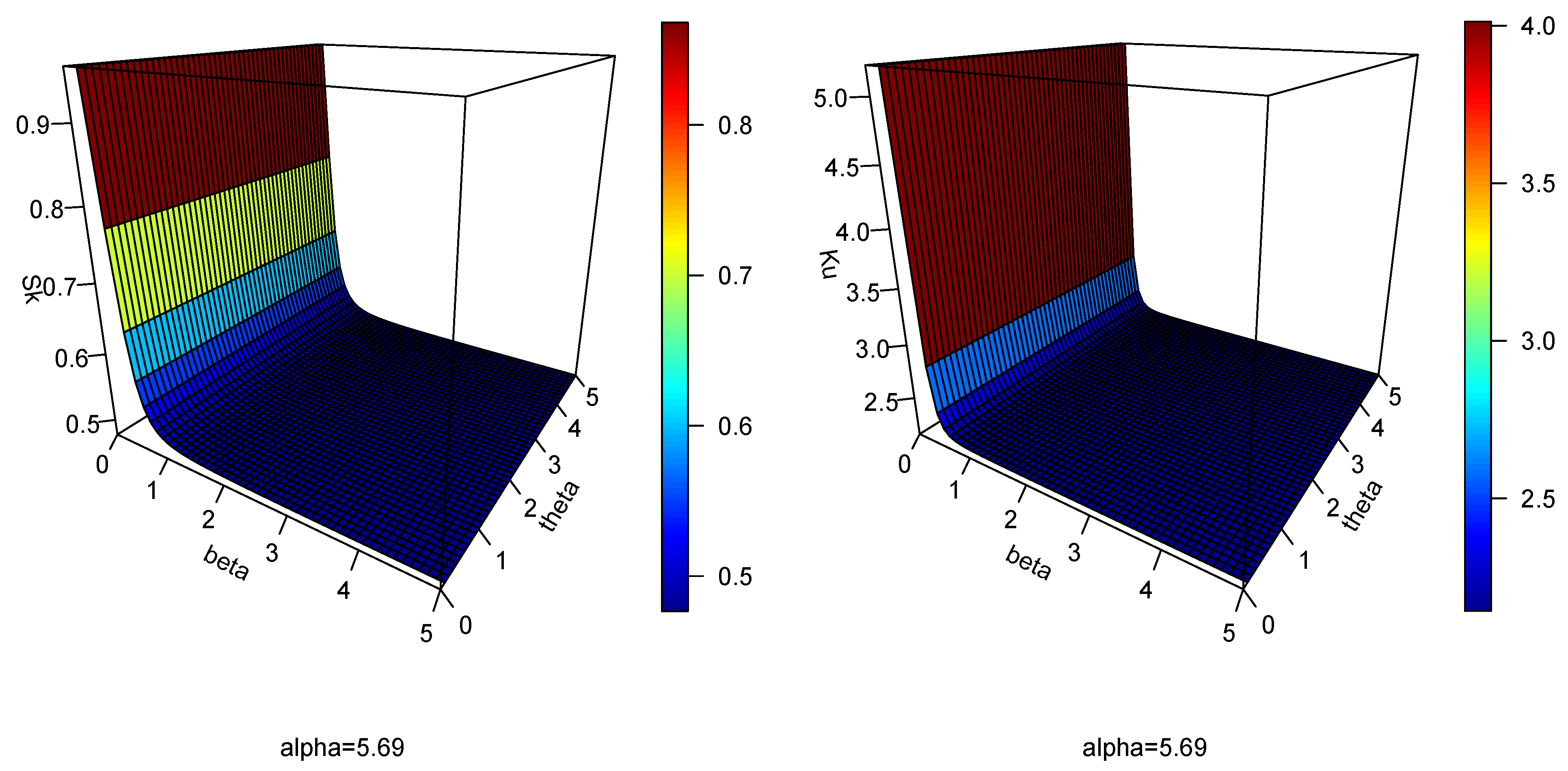
Measures for skewness (Sk) and kurtosis (Ku), QF-dependent, are sometimes more appropriate for the T-X family of distributions. The long tail degrees toward the left and right sides describe the skewness while the tail-heaviness degree describes kurtosis. When Sk $<0$ (or $>0$), the distribution is left- (or right)-skewed, and when Sk $=0$, the distribution is symmetric. The tail becomes heavier as Ku increases. Using QFs, Galton (1883) [13] and Moors (1988) [14] defined the skewness measure (Sk) and kurtosis measure (Ku), respectively, which are defined as follows

$$Sk=\frac{x_{0.75}+x_{0.25}-2x_{0.50}}{x_{0.75}-x_{0.25}}$$

and

$$Ku=\frac{x_{0.875}+x_{0.375}-(x_{0.625}+x_{0.125})}{x_{0.750}-x_{0.250}}$$

Figure 3 demonstrates the skewness and kurtosis plots of the EPAIG-ED.

Figure 3. Plots of Galton’s skewness (Sk) and Moor’s kurtosis (Ku) for the EPAIG-ED.

Simulation

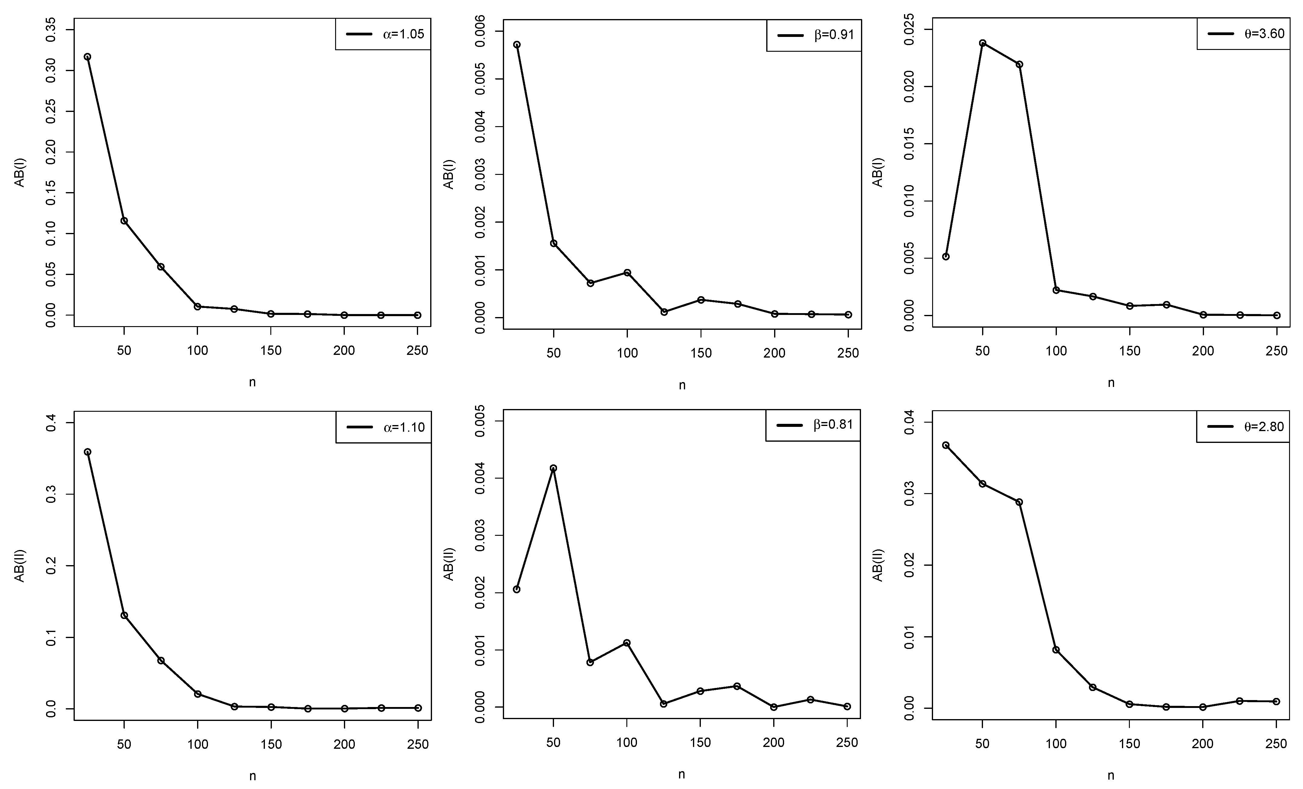
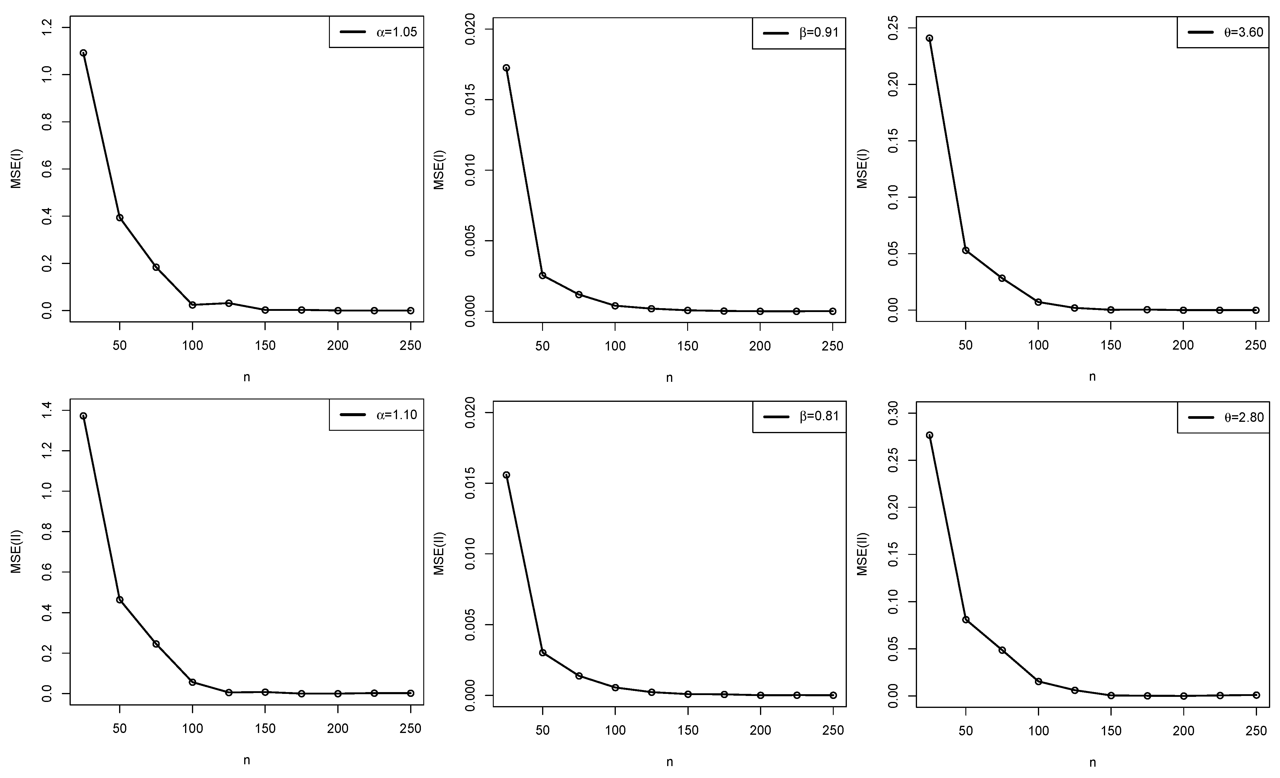
For the Monte Carlo (MC) simulation of the EPAIG-ED, from Equation (82) we consider that p is a uniform r.v. in (0,1). We simulate EPAIG-ED (for Set I: $\alpha =1.05,\beta =0.91,\theta =3.60$ and for Set II: $\alpha =1.10,\beta =0.81,\theta =2.80$) for $n=25,50,75,\cdots ,250$ times. For every sample size, we compute MLE for $\theta$, $\beta$, and $\alpha$. We consider 1000 MC replicates of this process and compute the average estimates (AEs), biases, absolute biases (ABs), and mean squares errors (MSEs). The results in Table 1 and displayed graphically in Figure 4 and Figure 5.

Table 1. The AEs, ABs, and MSEs based on 1000 MCSs of the EPAIG-ED.

Set I					Set II
$\mathit{\alpha }=\mathbf{1.05},\mathit{\beta }=\mathbf{0.91},\mathit{\theta }=\mathbf{3.60}$					$\mathit{\alpha }=\mathbf{1.10},\mathit{\beta }=\mathbf{0.81},\mathit{\theta }=\mathbf{2.80}$
n	Parameter	AEs	ABs	MSEs	AEs	ABs	MSEs
25	$\widehat{\alpha }$	1.366996	0.3169955	1.0929629	1.459311	0.3593107	1.3733343
	$\widehat{\beta }$	0.915721	0.0057207	0.0172636	0.812060	0.0020599	0.0155931
	$\widehat{\theta }$	3.605154	0.0051537	0.2410440	2.836797	0.0367966	0.2767344
50	$\widehat{\alpha }$	1.165887	0.1158869	0.3943543	1.231017	0.1310174	0.4650853
	$\widehat{\beta }$	0.908440	0.0015596	0.0025458	0.805823	0.0041773	0.0030314
	$\widehat{\theta }$	3.623810	0.0238105	0.0530842	2.831384	0.0313836	0.0811852
75	$\widehat{\alpha }$	1.109416	0.0594161	0.1839869	1.167718	0.0677182	0.2462002
	$\widehat{\beta }$	0.910724	0.0007236	0.0011887	0.810784	0.0007838	0.0013861
	$\widehat{\theta }$	3.621947	0.0219468	0.0283753	2.828831	0.0288310	0.0487680
100	$\widehat{\alpha }$	1.060522	0.0105221	0.0238978	1.120900	0.0208998	0.0568808
	$\widehat{\beta }$	0.909054	0.0009465	0.0003945	0.808874	0.0011265	0.0005601
	$\widehat{\theta }$	3.602222	0.0022217	0.0071837	2.808202	0.0082021	0.0154640
125	$\widehat{\alpha }$	1.057584	0.0075845	0.0312413	1.103230	0.0032299	0.0057049
	$\widehat{\beta }$	0.909879	0.0001209	0.0001872	0.809943	0.0000573	0.0002313
	$\widehat{\theta }$	3.601665	0.0016648	0.0019889	2.802945	0.0029449	0.0061457
150	$\widehat{\alpha }$	1.051616	0.0016164	0.0025074	1.102596	0.0025959	0.0078203
	$\widehat{\beta }$	0.910375	0.0003749	0.0000686	0.809719	0.0002812	0.0000922
	$\widehat{\theta }$	3.600837	0.0008371	0.0003068	2.800579	0.0005788	0.0006002
175	$\widehat{\alpha }$	1.051405	0.0014052	0.0026240	1.099661	0.0003391	0.0000959
	$\widehat{\beta }$	0.909711	0.0002891	0.0000212	0.809632	0.0003678	0.0000766
	$\widehat{\theta }$	3.600949	0.0009492	0.0004894	2.800197	0.0001968	0.0002496
200	$\widehat{\alpha }$	1.049917	0.0000833	0.0000029	1.099554	0.0004462	0.0000397
	$\widehat{\beta }$	0.909919	0.0000808	0.0000026	0.809998	0.0000016	0.0000143
	$\widehat{\theta }$	3.600068	0.0000677	0.0000039	2.800176	0.0001765	0.0000645
225	$\widehat{\alpha }$	1.050019	0.0000190	0.0000029	1.101291	0.0012907	0.0026624
	$\widehat{\beta }$	0.910074	0.0000735	0.0000028	0.809867	0.0001326	0.0000191
	$\widehat{\theta }$	3.599955	0.0000454	0.0000020	2.801026	0.0010258	0.0006225
250	$\widehat{\alpha }$	1.050028	0.0000280	0.0000008	1.101380	0.0013803	0.0023697
	$\widehat{\beta }$	0.910065	0.0000653	0.0000043	0.809987	0.0000127	0.0000164
	$\widehat{\theta }$	3.599985	0.0000152	0.0000002	2.800954	0.0009540	0.0010710

Figure 4. Plots of ABs based on the simulation of the EPAIG-ED for sets I and II.

Figure 5. Plots of MSEs based on the simulation of the EPAIG-ED for sets I and II.

Based on the empirical results of the simulation in Table 1, Figure 4, and Figure 5, we detect that the ABs and MSEs of MLEs $\theta$, $\beta$ and $\alpha$ decay toward zero as n increases. As n increases, the AEs are quite stable and tend to be close to actual parameter values. This reality assists the asymptotic normal distribution (ND) that gives an appropriate approximation to the finite sample distribution of estimates.

5.2. Estimation of the EPAIG-Exponential Model

The LLF for the sample size n with values $x_1,x_2,\cdots ,x_n$ of the EPAIG-E model for unknown parameters $\mathsf{\Phi }={(\theta ,\beta ,\alpha )}^T$ is

$$\begin{array}{cc}\hfill l& =l\left(\mathsf{\Phi }\right)=n[log\theta -\beta log(\alpha -1)+log\beta +log(log\alpha \left)\right]+\hfill \\ \hfill & (\beta -1)\sum _{i=1}^{n}log({\alpha }^{\frac{\theta x_i}{1+\theta x_i}}-1)+log\alpha \sum _{i=1}^n\frac{\theta x_i}{1+\theta x_i}-2\sum _{i=1}^{n}log(1+\theta x_i)\hfill \end{array}$$

(83)

Using the MML, the elements of the SFs $U\left(\mathsf{\Phi }\right)=(U_{\theta },U_{\beta },U_{\alpha })$ are given as

$$\begin{array}{cc}\hfill U_{\theta }=& \frac{n}{\theta }-2\sum _{i=1}^n\frac{x_i}{1+\theta x_i}+log\alpha \sum _{i=1}^n\frac{x_i}{{(1+\theta x_i)}^2}+\hfill \\ \hfill & (\beta -1)log\alpha \sum _{i=1}^n\frac{x_i}{{(1+\theta x_i)}^2(1-{\alpha }^{-\theta x_i{(1+\theta x_i)}^{-1}})}\hfill \end{array}$$

(84)

$$U_{\beta }=n\left[-log(\alpha -1)+\frac{1}{\beta }\right]+\sum _{i=1}^{n}log({\alpha }^{\theta x_i{(1+\theta x_i)}^{-1}}-1)$$

(85)

and

$$U_{\alpha }=n\left[{(\alpha log\alpha )}^{-1}-\beta {(\alpha -1)}^{-1}\right]+\frac{1}{\alpha }{\sum }_{i=1}^n\frac{\theta x_i}{\theta x_i+1}+(\beta -1){\sum }_{i=1}^n\frac{\theta x_i}{(\theta x_i+1)(\alpha -{\alpha }^{{(\theta x_i+1)}^{-1}})}$$

(86)

Setting, Equations (84)–(86) equate zero and solving simultaneously provide MLEs $\widehat{\mathsf{\Phi }}=(\widehat{\theta },\widehat{\beta },\widehat{\alpha })$ of $\mathsf{\Phi }$. Here, analytical solutions are tedious, therefore, we employ the fitdistrplus package using the R language to obtain the estimates.

5.3. Asymptotic Confidence Bounds of the EPAIG-ED

The large sample theory of ML estimators of the EPAIG-ED gives

$$\sqrt{n}({\widehat{\mathsf{\Phi }}}_i-{\mathsf{\Phi }}_i)\underrightarrow{d}{N}_3(0,I^{-1}({\widehat{\mathsf{\Phi }}}_i));i=\theta ,\beta ,\alpha$$

(87)

Here, $\underrightarrow{d}$ represents convergence in the distribution, $I_{ij}^{-1}\left(\widehat{\mathsf{\Phi }}\right)$ is a matrix of variability measures of the estimated parameters and is obtained from the inverse of the observed Fisher information matrix (OFIM) as approximated below

$$I_{ij}(\widehat{\mathsf{\Phi }})=E\left[-\frac{{\partial }^{2}l}{\partial {\mathsf{\Phi }}_i\partial {\mathsf{\Phi }}_j}{|}_{\mathsf{\Phi }=\widehat{\mathsf{\Phi }}}\right];i,j=\theta ,\beta ,\alpha$$

The large sample 100(1 − $\gamma$)% confidence intervals of $\widehat{\theta }$, $\widehat{\beta }$, and $\widehat{\alpha }$ of the EPAIG-ED are obtained, respectively, as

$${\widehat{\mathsf{\Phi }}}_i\pm Z_{\frac{\gamma }{2}}\sqrt{I^{-1}\left({\widehat{\mathsf{\Phi }}}_i\right)};i=\theta ,\beta ,\alpha$$

where $Z_{\frac{\gamma }{2}}$ is the upper $\frac{\gamma }{2}$th percentile of the standard ND. The derivatives in the OFIM w.r.t $\alpha$, $\beta$ and $\theta$ are obtained below

$$\begin{array}{cc}\hfill \frac{{\partial }^{2}l}{\partial {\alpha }^2}=& n\left[\frac{\beta }{{(\alpha -1)}^2}-\frac{1+log\alpha }{{(\alpha log\alpha )}^2}\right]-\frac{1}{{\alpha }^2}\sum _{i=1}^n\frac{\theta x_i}{1+\theta x_i}+\hfill \\ \hfill & (1-\beta )\sum _{i=1}^n\frac{\theta x_i}{(1+\theta x_i){(\alpha -{\alpha }^{{(1+\theta x_i)}^{-1}})}^2}\left[1-\frac{1}{1+\theta x_i}{\alpha }^{-\frac{\theta x_i}{1+\theta x_i}}\right]\hfill \end{array}$$

(88)

$$\frac{{\partial }^{2}l}{\partial \alpha \partial \beta }=-\frac{n}{\alpha -1}+\sum _{i=1}^n\frac{\left(\theta x_i\right){(\alpha -{\alpha }^{\frac{1}{1+\theta x_i}})}^{-1}}{(1+\theta x_i)}$$

(89)

$$\begin{array}{cc}\hfill \frac{{\partial }^{2}l}{\partial \alpha \partial \theta }& =(\beta -1)\sum _{i=1}^n\frac{x_i}{(\alpha -{\alpha }^{\frac{1}{1+\theta x_i}}){(1+\theta x_i)}^2}\left[1-\theta log\alpha \frac{x_i{\alpha }^{\frac{1}{1+\theta x_i}}}{(1+\theta x_i)(\alpha -{\alpha }^{\frac{1}{1+\theta x_i}})}\right]\hfill \\ \hfill & +\frac{1}{\alpha }\sum _{i=1}^n\frac{x_i}{{(1+\theta x_i)}^2}\hfill \end{array}$$

(90)

$$\frac{{\partial }^{2}l}{\partial {\beta }^2}=-\frac{n}{{\beta }^2}$$

(91)

$$\frac{{\partial }^{2}l}{\partial \beta \partial \theta }=log\alpha \sum _{i=1}^n{x}_i{\alpha }^{\frac{\theta x_i}{1+\theta x_i}}\frac{1}{({\alpha }^{\frac{\theta x_i}{1+\theta x_i}}-1){(1+\theta x_i)}^2}$$

(92)

$$\begin{array}{cc}\hfill \frac{{\partial }^{2}l}{\partial {\theta }^2}=& -\frac{n}{{\theta }^2}+(1-\beta )log\alpha \sum _{i=1}^n\frac{x_i^2}{(1-{\alpha }^{-\frac{\theta x_i}{1+\theta x_i}}){(1+\theta x_i)}^3}\left[\frac{log\alpha }{(1+\theta x_i)({\alpha }^{\frac{\theta x_i}{1+\theta x_i}}-1)}+2\right]\hfill \\ \hfill & +2\sum _{i=1}^n\frac{x_i^2}{{(1+\theta x_i)}^2}\left[1-\frac{log\alpha }{1+\theta x_i}\right]\hfill \end{array}$$

(93)

5.4. Applications

This section explains the illustration of the proposed model, the EPAIG-E model, by fitting it to a real dataset. The dataset, as reported by [15], describes one of the hydrological characteristics. The storm events with observations of water runoff (mm) from a watershed in Korea are as follows: 0.90, 0.60, 16.80, 59.30, 2.0, 78.20, 30.70, 146.80, 1.80, 3.40, 1.10, 0.80, 2.50, 6.10, 17.0, 5.10, 216.20, 8.10, 1.60, 2.0, 2.0, 0.80, 0.80, 2.90, 7.30, 13.30, 181.70, 20.50, 24.10, 33.50, 89.10, 7.20, 6.0, 75.90.

In the hydrological data analysis, the probability distribution models are as follows:

1.

Alpha power exponential (APE) [2]

$$g(\theta ,\alpha ;x)=\frac{\theta log\alpha }{\alpha -1}{\alpha }^{1-e^{-\theta x}}{e}^{-\theta x};\alpha ,\theta ,x>0,\alpha \ne 1$$

2.

Exponentiated alpha power exponential (EAPE)

$$g(\theta ,\alpha ,a;x)=\frac{a\theta log\alpha }{\alpha -1}{e}^{-\theta x}{\alpha }^{1-e^{-\theta x}}{\left(\frac{{\alpha }^{1-e^{-\theta x}}-1}{\alpha -1}\right)}^{a-1};\alpha \ne 1,a,\alpha ,\theta ,x>0$$

3.

Exponentiated exponential (EE) [3]

$$g(\theta ,\gamma ;x)=\gamma \theta {(1-e^{-\theta x})}^{\gamma -1}{e}^{-\theta x};\gamma ,\theta ,x>0$$

4.

Kumaraswamy exponential (KwE) [16]

$$g(\theta ,b,a;x)=ab\theta e^{-\theta x}{\left(1-e^{-\theta x}\right)}^{a-1}{\left(1-{\left(1-e^{-\theta x}\right)}^a\right)}^{b-1};\theta ,a,b,x>0$$

5.

Exponential (Exp.)

$$g(\theta ;x)=\theta e^{-\theta x};\theta ,x>0$$

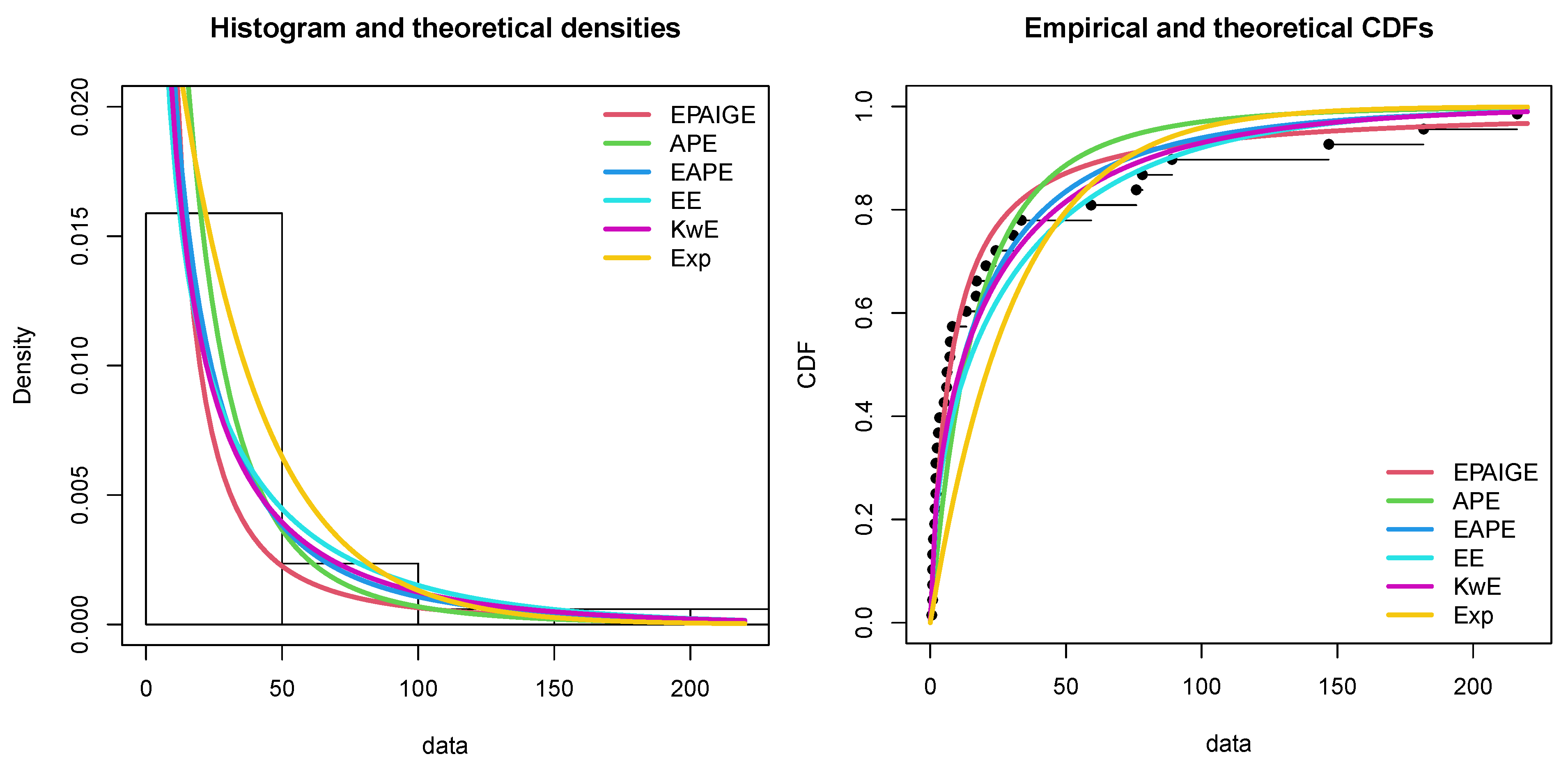
The EPAIG-E and all compared models were fitted to runoff data and the parameters using MML were estimated. The parameter estimates along with standard errors are given in Table 2. Further, the goodness of fit (GoF) test statistics criteria, such as negative log-likelihood-L, Bayesian information criterion (IC) (BIC), Akaike IC (AIC), Kolmogorov–Smirnov (KS), p-value, Anderson–Darling (AD), and Cramer-von Mises (CM) were used to check the performances of the fitting models for runoff data. The statistics were obtained for each model and are listed in Table 3. From Table 3, we observe that the EPAIG-E model has minimum values of GoF test statistics with large p-values. Further, plots in Figure 6 favor the EPAIG-E model. Accordingly, we can conclude that the EPAIG-E model is the best compared to other models for runoff data.

Table 2. Estimates and standard errors of parameters of the EPAIG-E model for runoff data.

Model	$\widehat{\mathit{\alpha }}$	$\widehat{\mathit{\beta }}$	$\widehat{\mathit{\theta }}$	$\widehat{\mathit{a}}$	$\widehat{\mathit{b}}$	$\widehat{\mathit{\gamma }}$
EPAIG-E	1.694325	0.970537	0.168391	–	–	–
	(2.513402)	(0.400538)	(0.002464)
APE	0.041160	–	0.018047	–	–	–
	(0.045367)		(0.005782)
EAPE	0.108038	–	0.012695	0.564599	–	–
	(0.176398)		(0.006486)	(0.132784)
EE	–	–	0.018009	–	–	0.460035
			(0.005133)			(0.092739)
KwE	–	–	0.003560	0.543711	3.622011	–
			(0.002083)	(0.089533)	(1.781159)
Exp.	–	–	0.031892	–	–	–
			(0.005464)

Table 3. The measures -L, AIC, BIC, KS, p-Value, CM, and AD for runoff data.

Model	-L	AIC	BIC	KS	p-Value	CM	AD
EPAIG-E	138.6977	283.3954	287.9745	0.1091	0.8129	0.084811	0.624680
APE	144.2117	292.4233	295.4760	0.2314	0.0524	0.530737	3.670699
EAPE	141.0578	288.1157	292.6948	0.1639	0.3207	0.195203	1.180785
EE	142.2647	288.5293	291.5821	0.1892	0.1752	0.271831	1.485958
KwE	140.9855	287.9711	292.5502	0.1569	0.3724	0.175093	1.075832
Exp.	151.1437	304.2873	305.8137	0.3606	0.0003	1.341393	9.032758

Figure 6. Histogram and estimated pdfs (left); empirical and estimated cdfs (right) of the EPAIG-E, APE, EAPE, EE, KwE, and Exp. models for the runoff data.

6. Conclusions

This article proposes a new family called the exponentiated power alpha index generalized-G. We used the new family to develop a new model of the three parameters—called the EPAIG-E model—to extend the exponential distribution. The EPAIG-E model is motivated by the wide application of the ED in analyzing lifetime datasets. We obtained structural properties of the EPAIG-G family. The parameter estimation of the EPAIG-G family and its model is obtained by MML. Simulation results are provided to assess the method’s performance. Real data applications of the proposed model fit relatively better than APE, EAPE, EE, KwE, and Exp.

References

- Gupta, R.C.; Gupta, P.L.; Gupta, R.D. Modeling failure time data by Lehman alternatives. Commun. Stat.-Theory Methods 1998, 27, 887–904. [Google Scholar] [CrossRef]
- Mahdavi, A.; Kundu, D. A new method for generating distributions with an application to exponential distribution. Commun. Statist. Theory Methods 2017, 46, 6543–6557. [Google Scholar] [CrossRef]
- Gupta, R.D.; Kundu, D. Exponentiated exponential family: An alternative to gamma and Weibull distributions. Biomed. J. 2001, 43, 117–130. [Google Scholar] [CrossRef]
- Tahir, M.H.; Nadarajah, S. Parameter induction in continuous univariate distributions: Well-established G families. Acad. Bras. Cienc. 2015, 87, 539–568. [Google Scholar] [CrossRef] [PubMed]
- ElSherpieny, E.A.; Almetwally, E.M. The Exponentiated Generalized Alpha Power Exponential Distribution: Properties and Applications. Pak. J. Stat. Oper. Res. 2022, 18, 349–367. [Google Scholar] [CrossRef]
- Hussain, S.; Sajid Rashid, M.; Ul Hassan, M.; Ahmed, R. The Generalized Exponential Extended Exponentiated Family of Distributions: Theory, Properties, and Applications. Mathematics 2022, 10, 3419. [Google Scholar] [CrossRef]
- Alzaatreh, A.; Lee, C.; Famoye, F. A new method for generating families of continuous distribution. Metron 2013, 71, 63–79. [Google Scholar] [CrossRef]
- Flajonet, P.; Odlyzko, A. Singularity analysis of generating function. SIAM J. Discr. Math. 1990, 3, 216–240. [Google Scholar] [CrossRef]
- Flajonet, P.; Sedgewich, R. Analytic Combinatorics; Cambridge University Press: Cambridge, UK, 2009; ISBN 978-0-521-89806-5. [Google Scholar]
- Rényi, A. On measures of entropy and information. Hung. Acad. Sci. 1961, 1, 547–561. [Google Scholar]
- Shannon, C.E. Prediction and entropy of printed Engish. Bell Syst. Tech. J. 1951, 30, 50–64. [Google Scholar] [CrossRef]
- Gradshteyn, I.S.; Ryzhik, I.M. Table of Integrals, Series, and Products, 7th ed.; Academic Press: San Diego, CA, USA, 2007. [Google Scholar]
- Galton, F. Enquiries into Human Faculty and its Development; Macmillan & Company: London, UK, 1883. [Google Scholar]
- Moors, J.J. A quantile alterrnative for kurtosis. Statistician 1988, 37, 25–32. [Google Scholar] [CrossRef]
- Hussain, S.; Rashid, M.S.; Ul Hassan, M.; Ahmed, R. The Generalized Alpha Exponent Power Family of Distributions: Properties and Applications. Mathematics 2022, 10, 1421. [Google Scholar] [CrossRef]
- Adepoju, K.A.; Chukwu, O.I. Maximum Likelihood Estimation of the Kumaraswamy Exponential Distribution with Applications. J. Mod. Appl. Stat. Methods 2015, 14, 208–214. [Google Scholar] [CrossRef]
Disclaimer/Publisher’s Note: The statements, opinions and data contained in all publications are solely those of the individual author(s) and contributor(s) and not of MDPI and/or the editor(s). MDPI and/or the editor(s) disclaim responsibility for any injury to people or property resulting from any ideas, methods, instructions or products referred to in the content. |
© 2023 by the authors. Licensee MDPI, Basel, Switzerland. This article is an open access article distributed under the terms and conditions of the Creative Commons Attribution (CC BY) license (https://creativecommons.org/licenses/by/4.0/).