Amplitude-Versus-Angle (AVA) Inversion for Pre-Stack Seismic Data with L0-Norm-Gradient Regularization

Abstract

Amplitude-versus-angle (AVA) inversion for pre-stack seismic data is a key technology in oil and gas reservoir prediction. Conventional AVA inversion contains two main stages. Stage one estimates the relative change rates of P-wave velocity, S-wave velocity and density, and stage two obtains the P-wave velocity, S-wave velocity and density based on their relative change rates through trace integration. An alternative way merges these two stages to estimate P-wave velocity, S-wave velocity and density directly. This way is less sensitive to noise in seismic data compared to conventional two-stage AVA inversion. However, the regularization for the direct AVA inversion is more complex. To regularize this merged inverse problem, the L0-norm-gradient of P-wave velocity, S-wave velocity and density was used. L0-norm-gradient regularization can provide inversion results with blocky features to make formation interfaces and geological edges precise. Then, L0-norm-gradient regularized AVA inversion was performed on the synthetic seismic traces. Next, a real seismic data line that contains three partial angle stack profiles was used to test the practice application. The inversion results from synthetic and real seismic data showed that L0-norm-gradient regularized AVA inversion is an effective way to estimate P-wave velocity, S-wave velocity and density.

1. Introduction

In exploration geophysics, the subsurface distribution of P-wave velocity, S-wave velocity and density of underground formation are frequently used to mark rock characteristics and help stratigraphic analysis. Amplitude-versus-angle (AVA) inversion is a way to estimate P-wave velocity, S-wave velocity and density from pre-stack seismic data. The inverted P-wave velocity, S-wave velocity and density can be used in rock characterization, stratigraphic correlation, lithology identification and further reservoir prediction, and many other areas in the oil and gas industry.

Zoeppritz’s equations are the theoretical foundation of AVA inversion [1,2,3]. The way to derive the exact analytic solution can be found in the literature [3]. However, the exact solution of Zoeppritz’s equations is too complicated to apply in practice. First, the analytical formulation of the exact solution is tedious, i.e., the analytic solution exists but is too complicated to write it mathematically. Second, the computation cost is relatively high. Numerically calculating the analytical solution is more computationally expensive than finding the solution of the linear system under analysis. To simplify the solution, many scholars derived different approximate expressions. For example, under the assumption of small changes in elastic parameters, Aki and Richards derived the approximate expression of the P-wave reflection coefficient with the relative variation rates of P-wave velocity, S-wave velocity, and density [3]. Additionally, there are many other approximate expressions in terms of different parameters. For example, Li and Zhang used the P-σ-ρ approximate expression to estimate Poisson’s ratio through AVA inversion (P is shorthand for P-wave velocity, σ is Poisson’s ratio, and ρ is density) [4].

Extending the approximate expression or exact solution of the P-wave reflection coefficient to M incident angles and N time samples at each common midpoint (CMP) and combining the convolution model of seismic data, one can obtain the forward problem of conventional AVA inversion, i.e., modeling seismic data according to given P-wave velocity, S-wave velocity and density model. Hence, AVA inversion estimates the model parameters of the subsurface from observed seismic data. However, it is not to say that the works of AVA inversion are easy. First, pre-stack seismic data are band limited and contain much noise. The forward operator of AVA inversion has a high condition number. All of these reasons cause the ill-posedness of AVA inversion. Hence, some a priori constraints to serve as the regularization term need to be introduced to obtain a stable and meaningful inversion result [5,6]. Regularization can alleviate the ill-posedness of an inverse problem.

Regularization considers the properties of the forward operator from the mathematical viewpoint [2]: Whether the numerical instability comes from the singularity and whether the singular operator can be modified to stabilize the computation. The stability means that a small variation in data causes a small perturbation in solution estimate and thus depends on the property of the forward operator [7]. There are three types of dependencies: linear, power law, and logarithmic [2]. With a linear dependency, it is a well-posed problem. For logarithmic dependency, it is an ill-posed problem. In order to have a stable inversion, at least an operator of power-law dependency, with an exponent less than 1, should be employed. Unfortunately, the operators in seismic inversion problems, especially for AVA inversion, are usually ill-posed with a logarithmic dependency [2].

The first used regularization method in geophysical inverse problems is Tikhonov regularization, which is the L2-norm of the model parameter or its attributes [7,8]. From the point of view of Bayesianism, the Tikhonov regularization corresponds to a priori Gaussian distribution of model parameters. In many alternative options, sparse regularization was very popular and frequently used to constrain AVA inversion to obtain sparse relative variation rates, which can further obtain blocky inversion results. Downton and Downton et al. performed AVA inversion regularized by three different sparse norms, i.e., Lp-norm, Cauchy’s norm, and Huber’s norm [5,6]. Alemie and Sacchi used Trivariate Cauchy probability distribution as the a priori constraint in three-term AVA inversion [9]. Zhang and Dai adopted Cauchy’s regularization to constrain AVA inversion and used a quasi-Newton algorithm to solve the objective function [10]. However, the sparse constraints on the relative variation rates will suppress some small reflection events overwhelmed by noise and cannot well estimate weak reflectors [11,12,13,14].

The existing AVA inversion methods usually involve two main stages. First, one can invert pre-stack seismic data to obtain the relative change rates of P-wave velocity, S-wave velocity and density; this is stage one. Next, the final P-wave velocity, S-wave velocity and density can be estimated based on the inverted relative change rates under trace integration transformation [10,15]; this is stage two.

The inversion methods with two stages have been used to solve most of the problems in AVA inversion. However, some issues remain. The results of the trace integration are sensitive to noise in the pre-stack seismic data and inaccuracies in the estimated relative change rates from stage one [16,17]. To reduce the ill-posedness of AVA inversion, the two-stage inverse problems can be merged into a single problem to estimate P-wave velocity, S-wave velocity and density directly. It is similar to the merged seismic impedance inversion methods proposed by the existing literature [17,18,19,20,21].

The merged inversion methods are less sensitive to noise compared to conventional two-stage AVA inversion. However, the regularization for direct inversion is more complex. In direct seismic impedance inversion, Gholami used total variation as the regularization term in the direct impedance inversion objective function to obtain impedance with blocky structures [17]. Hamid and Pidlisecky used a damped least-squares method to estimate the impedance model [18]. Yuan et al. used a transform-domain sparsity promotion method to address the seismic impedance inversion [19]. Yang et al. and Dai et al. used L0-norm-gradient as the regularization term in the direct impedance inversion and compared the L0-norm-gradient regularized impedance inversion to the other existing inversion methods [20,21]. They pointed out the advantages of L0-norm-gradient regularization in seismic impedance inversion. At first, L0-norm regularization is used to constrain the representation coefficients in the sparse signal representation and compressed sensing theory [22,23]. Xu et al. used the idea of the L0-norm-gradient for image smoothing [24]. Cheng et al. extended Xu et al.’s work to preserve the image’s features in image processing [25].

In this paper, we applied the L0-norm-gradient of P-wave velocity, S-wave velocity and density in direct AVA inversion to regularize the merged inverse problem. In AVA inversion, L0-norm-gradient regularization can provide inversion results with blocky features to make formation interfaces and geological edges precise. However, to adapt the specific feature of AVA inversion, we modified the conventional form of L0-norm-gradient by introducing the inverse of covariance matrix between P-wave velocity, S-wave velocity and density to serve as a weighting matrix for model parameters to consider the statistical correlation between them. To solve the L0-norm-gradient regularized AVA inversion, a split-Bregman-like algorithm was used. Then, L0-norm-gradient regularized AVA inversion was performed on the synthetic seismic traces. Next, a real seismic data line that contains three partial angle stack profiles was used to test the practice application. The inversion results from synthetic and real seismic data showed that L0-norm-gradient regularized AVA inversion is an effective way to estimate P-wave velocity, S-wave velocity and density.

2. Methods

2.1. AVA Inversion for Pre-Stack Seismic Data

Here, we used the approximate expression of the P-wave reflection coefficient derived by Aki and Richards with relative variation rates of P-wave velocity, S-wave velocity and density to construct the objective function of AVA inversion. The Aki–Richards approximation can be expressed as [3]

$$R_{pp}(\theta )\approx a(\theta )R_{vp}+b(\theta ,\gamma )R_{vs}+c(\theta ,\gamma )R_{\rho },$$

(1)

where R_pp(θ) is the P-wave reflection coefficient at incident angle θ; $a(\theta )={\sec }^2\theta$; $b(\theta ,\gamma )=-8{\gamma }^2{\sin }^2\theta$; $c(\theta ,\gamma )=(1-4{\gamma }^2{\sin }^2\theta )$; γ is the ratio of background S-wave velocity to P-wave velocity; and R_vp, R_vs and R_ρ are the relative variation rates of P-wave velocity, S-wave velocity and density, respectively.

We assumed that the pre-stack seismic data contains M incident angles and N time samples at each CMP. Hence, Equation (1) can be extended to the following form [10]:

$$r_{pp}=Ar,$$

(2)

where $r_{pp}\in R^{MN}$ is the vector of the P-wave reflection coefficient at M incident angles and N time samples; $r\in R^{3N}$ is the vector of the relative variation rates of P-wave velocity, S-wave velocity and density at N time samples; and $A\in R^{MN\times 3N}$ is the matrix which is constituted by a(θ), b(θ) and c(θ) at M incident angles [10], i.e.,

$$r_{pp}={[R_{pp}^1({\theta }_1),\dots ,R_{pp}^N({\theta }_1),\dots ,R_{pp}^1({\theta }_M),\dots ,R_{pp}^N({\theta }_M)]}^T$$

(3)

$$r={[R_{vp}^1,\dots ,R_{vp}^N,R_{vs}^1,\dots ,R_{vs}^N,R_{\rho }^1,\dots ,R_{\rho }^N]}^T$$

(4)

$$A=\left[\begin{array}{ccccccccc}a({\theta }_1)& & & b({\theta }_1)& & & c({\theta }_1)& & \\ & \dots & & & \dots & & & \dots & \\ & & a({\theta }_1)& & & b({\theta }_1)& & & c({\theta }_1)\\ & \dots & & & \dots & & & \dots & \\ a({\theta }_M)& & & b({\theta }_M)& & & c({\theta }_M)& & \\ & \dots & & & \dots & & & \dots & \\ & & a({\theta }_M)& & & b({\theta }_M)& & & c({\theta }_M)\end{array}\right]$$

(5)

In exploration geophysics, we think the observed seismic data are the convolution result from the P-wave reflection coefficient and a source wavelet [26]. For calculation, the convolution relationship is discretized as

$$d=W{r}_{pp}+n$$

(6)

where $d\in R^{MN}$ is the vector of observed pre-stack seismic data at each CMP; $n\in R^{MN}$ is the noise in observed seismic data; and $W\in R^{MN\times MN}$ is the wavelet convolution matrix for pre-stack seismic data, in which each column contains the wavelet properly padded with zeros in order to express discrete convolution [2].

Hence, it is assumed that the observed data d are well described by the synthetic data given by Wr and an additive noise n in this paper.

By combining Equations (2) and (6), one can obtain the forward equation for the conventional two-stage AVA inversion, i.e.,

$$d=WAr+n=\Phi r+n,$$

(7)

where Φ = WA$\in R^{MN\times 3N}$, which is the combined matrix of W and A and serves as the forward operator of conventional AVA inversion.

Based on the least square inverse problem theory, the objective function of AVA inversion can be written as

$$\min f(r)=\left|\right|\Phi r-d|{|}_2^2,$$

(8)

where $\left|\right|\cdot |{|}_2$ is the L2-norm of a vector.

However, the solution of seismic inversion is ill-posed. To alleviate the ill-posed inverse problem, the most effective way is the regularization constraint [8]. In a seismic inversion, sparse regularization is very popular and has frequently been used to constrain AVA inversion to obtain sparse relative variation rates, which can further obtain blocky inversion results. Here, we used L0-norm as the sparse regularization. Hence, the objective function of AVA inversion with L0-nom sparse regularization is

$$\min f(r)=\left|\right|\Phi r-d|{|}_2^2+\lambda |\left|r\right|{|}_0,$$

(9)

where $\left|\right|\cdot |{|}_0$ is the so-called L0-norm of a vector, i.e., the number of no-zero elements in a vector; $\lambda$ is the regularization parameter of L0-nom sparse regularization. Equation (6) is the so-called sparse spike seismic inversion [27].

After establishing the solution to Equation (6), i.e., the inverted relative variation rates, the final P-wave velocity, S-wave velocity and density can be obtained through the following trace integration transformation [10,15], i.e.,

$$\{\begin{array}{l}vp(i)=vp(0)\exp [2{\displaystyle \sum _{j=0}^i{R}_{vp}^j]}\\ vs(i)=vs(0)\exp [2{\displaystyle \sum _{j=0}^i{R}_{vs}^j]}\\ \rho (i)=\rho (0)\exp [2{\displaystyle \sum _{j=0}^i{R}_{\rho }^j]}\end{array},$$

(10)

where vp(i), vs(i) and ρ(i) are P-wave velocity, S-wave velocity and density at sample i, respectively.

2.2. L0-Norm-Gradient Regularization

For continuous model parameters m(x), its L0-norm can be defined as the length of its support set, i.e., [7]

$$\left|\right|m\left|{|}_0=|\mathrm{spt}m\right|,$$

(11)

where sptm is the support set of m(x).

Hence, the L0-norm can also be expressed as

$$\left|\right|m|{|}_0={\displaystyle {\int }_{x\in \mathrm{V}}l[m(x)]\mathrm{d}x},$$

(12)

where

$$l(m)=\{\begin{array}{l}1\hspace{1em}m\ne 0\\ 0\hspace{1em}m=0\end{array},$$

(13)

From the above definition, for the discretized model parameters m, its L0-norm can be expressed as [12]

$$\left|\right|m\left|{|}_0=\text{{}\mathrm{the}\mathrm{total}\mathrm{number}\mathrm{of}i\right|m\left(i\right)\ne 0\text{}},$$

(14)

where m(i) is the element of m.

Based on the definition (11), the L0-norm-gradient of model parameters m(x) can be defined as

$$\left|\right|\nabla m|{|}_0=|\mathrm{spt}\nabla m|,$$

(15)

For the special case of seismic inversion in one dimensional, such as seismic impedance inversion trace by trace or AVA inversion performed CMP by CMP, the gradient of model parameters is the partial derivative in a vertical direction, i.e.,

$$\left|\right|\nabla m|{|}_0=|\left|{\partial }_{z}m\right|{|}_0,$$

(16)

Hence, for the discretization one-dimensional case, the L0-norm-gradient can be expressed as [20,21]

$$\left|\right|\nabla m|{|}_0=|\left|Dm\right|{|}_0,$$

(17)

where D is the first-order difference operator matrix.

From the definition of L0-norm-gradient, we can see that it measures the sparsity of the model parameters’ gradient. Applying L0-norm-gradient as a regularization in seismic inversion can provide inversion results with blocky features to make formation interfaces and geological edges precise. In fact, the L0-norm gradient is the extension of the total variation. L0-norm-gradient use L0-norm to replace L1-norm in the definition of the total variation. Compared to other measures of sparsity, L0-norm is the most essential one. It is because the other sparsity measures, such as L1-norm, Cauchy norm, Huber norm, Lp-norm (0 < p < 1), and so forth, are relaxations of L0-norm to a varying degree [12].

2.3. AVA Inversion with L0-Norm-Gradient Regularization

In a seismic inversion, the definition of the relative change rate of P-wave velocity can be expressed as [3]

$$R_{vp}^i\approx \frac{\Delta vp(i)}{2vp(i)}\approx \frac{1}{2}\ln \frac{vp(i+1)}{vp(i)}.$$

(18)

Considering there are N time samples at each CMP, Equation (18) can be extended to the following form:

$$R_{vp}=Du,$$

(19)

where R_vp$\in R^N$ represents the vector of relative variation rates of P-wave velocity at N samples, i.e.,

$$R_{vp}={[R_{vp}^1,\dots ,R_{vp}^N]}^T,$$

(20)

u$\in R^N$ is the vector with the following elements:

$$u(i)=(1/2)\ln \frac{vp(i)}{vp(0)},$$

(21)

Hence, u is the vector of logarithmic P-wave velocity.

Similarly, for the relative change rates of S-wave velocity and density, we have the following equations:

$$\{\begin{array}{l}{R}_{vs}=Dv\\ R_{\rho }=Dw\end{array},$$

(22)

where R_vs$\in R^N$ and R_ρ$\in R^N$ represent the vector of relative variation rates of S-wave velocity and density at N samples, and v$\in R^N$ and w$\in R^N$ are the vectors of logarithmic S-wave velocity and density, respectively.

By combining R_vp, R_vs and R_ρ, one can obtain r in Equation (2) and give the following equation:

$$r=Dm.$$

(23)

Now, m$\in R^{3N}$ is the vector combined u, v and w, and D$\in R^{3N\times 3N}$ represents a combined difference matrix for u, v and w.

By combining Equations (7) and (23), one can obtain the following equation:

$$d=Gm+n,$$

(24)

where G = ΦD$\in R^{MN\times 3N}$, which is the combined matrix of Φ and D.

In the above formula, Gm is the forward equation for the merged AVA inversion, and m is the model parameters. Based on Equation (24), we can directly estimate P-wave velocity, S-wave velocity and density.

Based on the objective function (9) for conventional AVA inversion, we can obtain the objective function for direct AVA inversion in the following form:

$$\min f(m)=\left|\right|Gm-d|{|}_2^2+\lambda |\left|Dm\right|{|}_0,$$

(25)

From the section on L0-norm-gradient regularization, we can see that Equation (25) is, in fact, an inverse problem regularized by L0-norm-gradient.

In direct AVA inversion, the model parameters m contains logarithmic P-wave velocity, logarithmic S-wave velocity and logarithmic density. Generally, there are correlations between different parameters. In addition, the contributions from the relative change rates of different parameters to the P-wave reflection coefficient are different. Compared to the relative change rates of P-wave velocity and S-wave velocity, the contribution from the relative change rate of density is very small [5]. Hence, the estimation of density is extremely unstable. To deal with this issue in AVA inversion, we can introduce a weighting matrix W_m$\in R^{3N\times 3N}$ for model parameters.

Furthermore, the pre-stack seismic data originate from different incident angles with different quality. For example, seismic data with large incident angles, which correspond to far offset, suffer different degrees of distortion due to NMO stretching [28]. Hence, the quality of seismic data with small incident angles is better compared to large incident angles. To deal with this issue in AVA inversion, we can also introduce a weighting matrix W_d$\in R^{MN\times MN}$ for seismic data.

By combining W_m and W_d, the objective function (25) can be updated as

$$\min f(m)=\left|\right|W_d(Gm-d)|{|}_2^2+\lambda |\left|D{W}_{m}m\right|{|}_0,$$

(26)

In AVA inversion, W_m and W_d usually take the following forms [9]:

$$\{\begin{array}{l}{W}_m=C_m^{-1}\\ W_d=C_d^{-1}\end{array},$$

(27)

where C_m$\in R^{3N\times 3N}$ and C_d$\in R^{MN\times MN}$ are the covariance matrix of model parameters and seismic data, respectively.

The covariance matrix C_d can be obtained from the observed pre-stack seismic data through statistical estimation. The covariance matrix C_m can be obtained from well log data or by means of empirical petrophysical relationships between model parameters [5,6]. For example, the Gardner formula represents the statistical relation between P-wave velocity and density [29], the Castagna formula represents the statistical relation between P-wave velocity and S-wave velocity [30], etc.

In fact, we can update the weighting matrix W_m at each iteration using inverted model parameters from the last iteration. This is the so-called strategy of iterative re-weighting, and AVA inversion becomes a nonlinear problem. However, the computational cost has increased accordingly.

2.4. Split-Bregman-like Algorithm

We used a split-Bregman-like algorithm to solve the objective function (26). First, introduce an auxiliary vector a$\in R^{3N}$; hence, the objective function (26) can be re-written as

$$\min f(m,a)=\left|\right|W_d(Gm-d)|{|}_2^2+\lambda |\left|a\right|{|}_0,\mathrm{s}.\mathrm{t}.a=D{W}_{m}m,$$

(28)

The above objective function can be written in Lagrangian form, i.e.,

$$\min f(m,a)=\left|\right|W_d(Gm-d)|{|}_2^2+\lambda |\left|a\right|{|}_0+{\mathsf{\beta }}^T(D{W}_{m}m-a),$$

(29)

where β $\in R^{3N}$ can be interpreted as a Lagrangian multiplier vector.

The Lagrangian imposes the strict constraint of equality, which is overkill [31]. In practice, one only needs to use the so-called augmented Lagrangian form, where the equality constraint is relaxed [31], i.e.,

$$\min f(m,a)=\left|\right|W_d(Gm-d)|{|}_2^2+\lambda |\left|a\right|{|}_0+\beta \left|\right|D{W}_{m}m-a|{|}_2^2.$$

(30)

Now, β is an auxiliary parameter similar to the regularization parameter but to control the similarity between the auxiliary vector a and DW_mm.

From the theory of the split-Bregman algorithm, Equation (30) asymptotically converges to Equation (29) as the auxiliary parameter β gradually increases [24,31,32]. Therefore, the value of β is varied; usually, it is kept low initially, but as the solution converges, its value is progressively increased.

The split-Bregman-like algorithm splits Equation (30) into two sub-problems and then iteratively solves them to find the solution of the original objective function [31]. Specifically, Equation (30) is solved iteratively by alternatively minimizing a and m. In each sub-problem, one variable is fixed with values obtained from the previous iteration.

Sub-problem 1: take a fixed and estimate m. The objective function for sub-problem 1 takes the following form:

$$\min f(m)=\left|\right|W_d(Gm-d)|{|}_2^2+\beta ||D{W}_{m}m-a|{|}_2^2.$$

(31)

It is an inverse problem regularized by quadratic regularization. Its solution is

$$m={(G^T{W}_d^T{W}_{d}G+\beta D^T{W}_m^{T}D{W}_m)}^{-1}(G^T{W}_d^{T}d+\beta D^T{W}_m^{T}a).$$

(32)

Sub-problem 2: take m fixed and update a. The objective function for sub-problem 2 takes the following form:

$$\min f(a)=\left|\right|D{W}_{m}m-a|{|}_2^2+\frac{\lambda }{\beta }|\left|a\right|{|}_0.$$

(33)

Equation (33) is a standard L0-norm regularized problem that can be solved by hard thresholding [31]. Its solution is

$$a(i)=\{\begin{array}{l}0,\hspace{1em}[(D{W}_{m}m)(i){]}^2\le \lambda /\beta \\ (D{W}_{m}m)(i),\hspace{1em}[(D{W}_{m}m)(i){]}^2>\lambda /\beta \end{array}.$$

(34)

where a(i) and (DW_mm)(i) are the ith element of a and DW_mm, respectively.

In the iteration, the auxiliary parameter β is automatically adapted starting from an initial value, and it is multiplied by κ each time [24].

After finding out the solution of the objective function (26) through the split-Bregman iteration algorithm, the final P-wave velocity, S-wave velocity and density can be obtained through the following simple exponential transformation [17], i.e.,

$$\{\begin{array}{l}vp(i)=vp(0)\exp [2u(i)]\\ vs(i)=vs(0)\exp [2v(i)]\\ \rho (i)=\rho (0)\exp [2w(i)]\end{array}.$$

(35)

We can see that the above Equation (35) is different from Equation (10). Equation (35) does not contain integration calculation. Hence, it is less sensitive to noise in seismic data.

3. Synthetic Data Tests

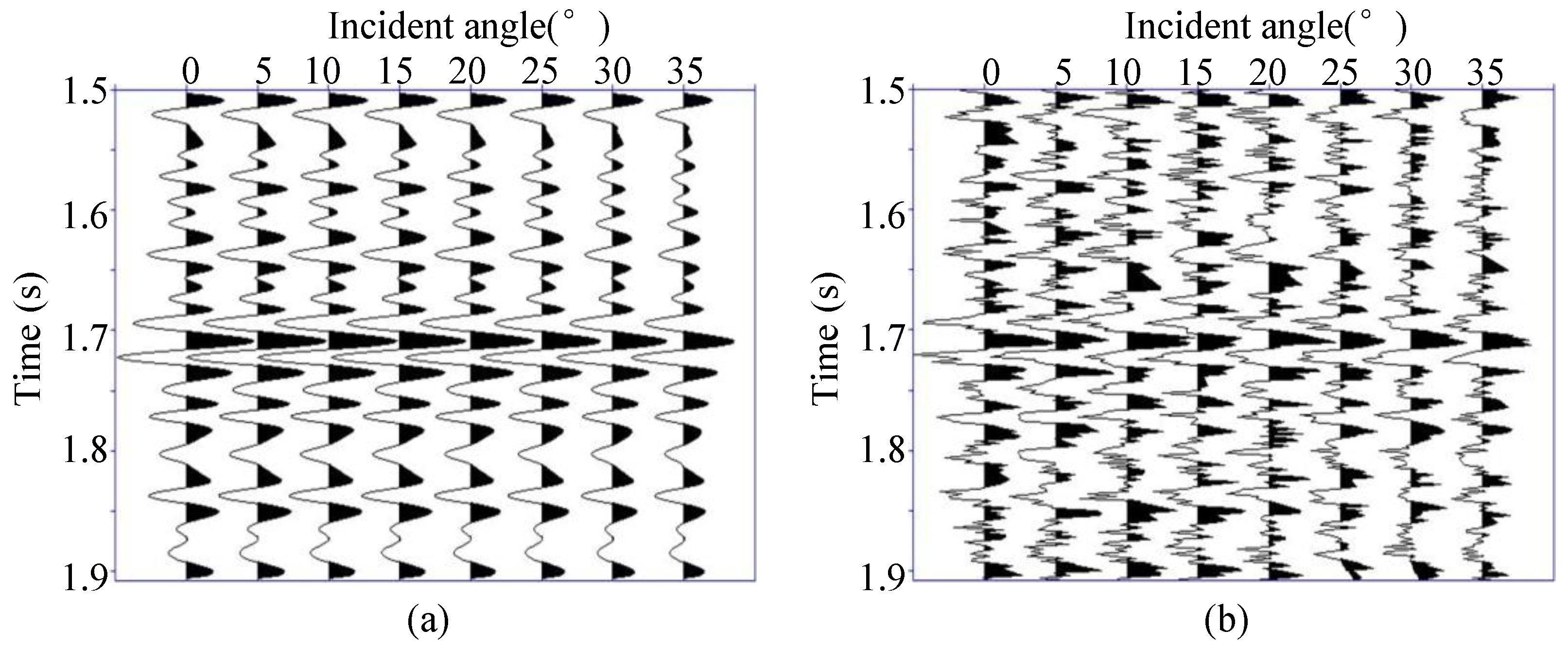
We first used the synthetic seismic traces to test the effects of AVA inversion with L0-norm-gradient regularization and its difference compared to conventional AVA inversion. The noise-free synthetic seismic traces are shown in Figure 1a, which are obtained from the convolution between a 35 Hz Ricker wavelet and the P-wave reflection coefficients with eight incident angles. The P-wave reflection coefficients are calculated from the P-wave velocity, S-wave velocity and density shown in with red curves through the Aki–Richards approximation. The eight incident angles are 0°, 5°,10°, 15°, 20°, 25°, 30° and 35°. Then, 25% zero-mean Gaussian random noise is added to the noise-free synthetic seismic traces. The noise-contaminated synthetic seismic traces are shown in Figure 1b. The relative error of the noise-contaminated data is 0.07.

Two AVA inversion methods were performed on the noise-contaminated synthetic seismic traces. The first one is conventional AVA inversion with sparse regularization (C-AVA), i.e., first, invert noise-contaminated synthetic seismic traces to obtain relative change rates, then estimate final P-wave velocity, S-wave velocity and density through trace integration transformation; the second one is direct AVA inversion with L0-norm-gradient regularization (L0-AVA).

In the process of AVA inversion, the initial model is the result of smoothing true model parameters through a high-cut filter with a threshold value of 10 Hz. We used quality control to calculate the regularization parameters in this paper. In synthetic data, the best value of regularization parameters is determined by quality control using a part of true model parameters; i.e., adjust the value of regularization parameters, obtain the inversion result with the corresponding part of seismic data for each set of regularization parameters, and choose the one whose inversion result has the best match with the true model parameters. From quality control, the regularization parameter λ is set to 0.1. The initial auxiliary parameter β is set to 2.0λ, and multiplier κ is set to 1.5. Then, the chosen regularization parameters are adopted when we perform inversion for the whole seismic data. The quality control part is a time interval of 1.55 s to 1.65 s. In addition, we used the true model parameters and seismic data in this time interval to calculate the model covariance matrix C_m and data covariance matrix C_d. The inverse of these two covariance matrices is served as the weighting matrices.

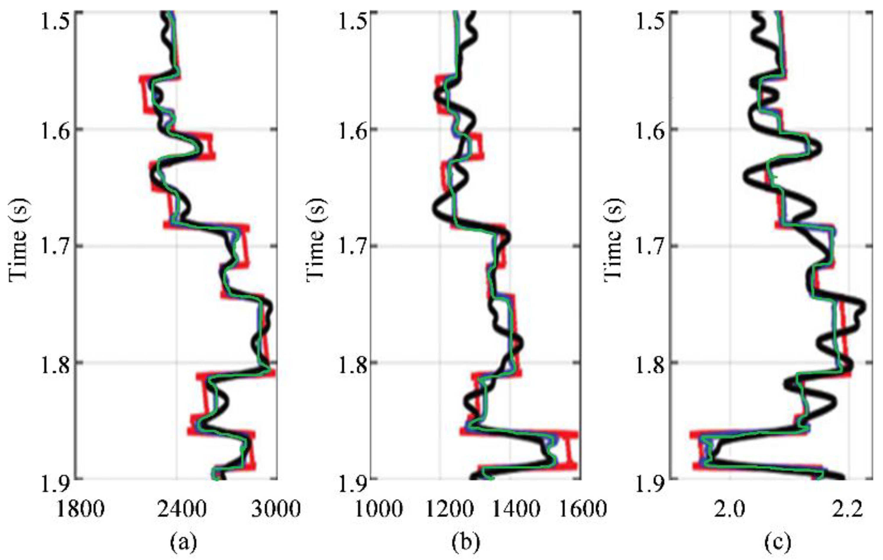
The inverted model parameters are shown in Figure 2, where the green curves are inverted model parameters by L0-AVA inversion, and the black curves are inverted model parameters by C-AVA inversion. Figure 2a–c shows P-wave velocity, S-wave velocity and density, respectively. Generally speaking, we can see that all of the inverted model parameters can match with the true model parameters and are following the relative trend of true model parameters very nicely. However, the inverted model parameters by the two AVA inversion methods are very different in detail. First, the inverted model parameters by C-AVA swings at some major large contrast interfaces. Especially below the time 1.7 s, the inverted model parameters by C-AVA inversion are very different from the true model parameters because the trace integration generates a large accumulation of errors. The formation boundary of the main stratigraphic sequence interface is not precise. Second, compared to C-AVA inversion, the inverted model parameters by L0-AVA inversion are better matched with true model parameters and have obvious “blocky” geological characteristics, with only small vibrations at contrast interfaces. Hence, the inverted model parameters by L0-AVA inversion are more accurate with higher resolution.

We calculated the relative errors (RE) of inverted model parameters by different AVA inversion methods through the following formula:

$$RE=\frac{\left|\right|m-m_{\mathrm{inverted}}|{|}_2^2}{\left|\right|m|{|}_2^2},$$

(36)

where $m_{\mathrm{inverted}}$ is inverted model parameters, and m is true model parameters. The calculated REs of inverted model parameters shown in Figure 2 are listed in

Table 1. The REs of inverted model parameters by different AVA inversion methods.

Inversion Method	RE
C-AVA	0.2223
L0-AVA	0.1305

. We can see that the RE for L0-AVA is much smaller than for C-AVA.

4. Field Data Applications

After performing synthetic seismic traces tests of L0-AVA inversion, a real seismic line from East China was used to test its practice application. The seismic data have a good signal-to-noise ratio, with signals extending from 10 to 120 Hz. The calculated relative error for this seismic line through the method proposed in the literature [33] is 0.22. 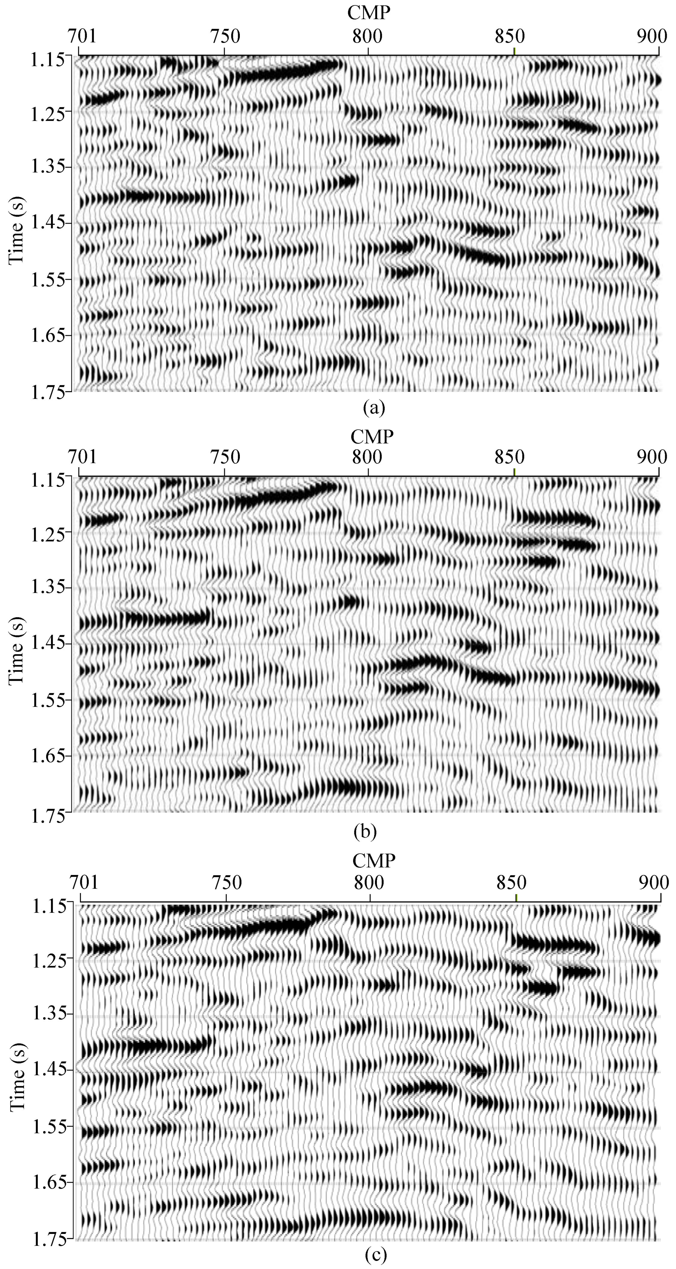The source wavelet was estimated from seismic-to-well correlation with a 50 Hz dominant frequency [2]. Before AVA inversion, the original seismic data were subjected to a suite of relative amplitude processing. The processing procedures contain shot and trace edits, noise attenuation, Q compensation, divergence correction, consistent surface scaling, consistent surface deconvolution, migration, residual statics, amplitude preserving NMO, multiple attenuations, transmission loss correction, etc. From the results of seismic processing for this line, we obtained three partial angle stack seismic data profiles, with stack angle ranges 2–11°, 12–21° and 22–31°, respectively. Figure 3 shows these three real partial angle stack seismic data profiles. The CMP numbers are from 701 to 900. These profiles show similar tectonic structures but with amplitude variations with stack angles. The amplitude variations are key information in AVA inversion.

Then, L0-AVA inversion is performed on this seismic data line. In the process of inversion, the initial model is obtained through the following procedures. First, we used local kriging estimation with P-wave velocity, S-wave velocity and density curves from a well log, which crosses this seismic line, under the constraint of seismic interpretation horizons to obtain well log interpolating models. Next, the interpolating model parameters models were smoothed through a high-cut filter with 10 Hz threshold value. The results are well log interpolating models with the low-frequency trend, which are used by us as the initial model. Additionally, we used quality control to determine these regularization parameters for field data inversion. Here, we think the actual well logs are the “answer” to the inversion of near-well seismic traces. The actual well logs represent the actual subsurface geological setting. The best value of regularization parameters is determined by quality control at well locations. From quality control for field data, the regularization parameter λ was set to 0.25. Same as synthetic data tests, the initial auxiliary parameter β was set to 2.0λ, and multiplier κ was set to 1.5. Then, the chosen regularization parameters were adopted when we performed inversion for other seismic traces. In addition, we used the actual well logs and near-well seismic traces to calculate model covariance matrix C_m and data covariance matrix C_d, and the inverse of these two covariance matrices was served as the weighting matrices.

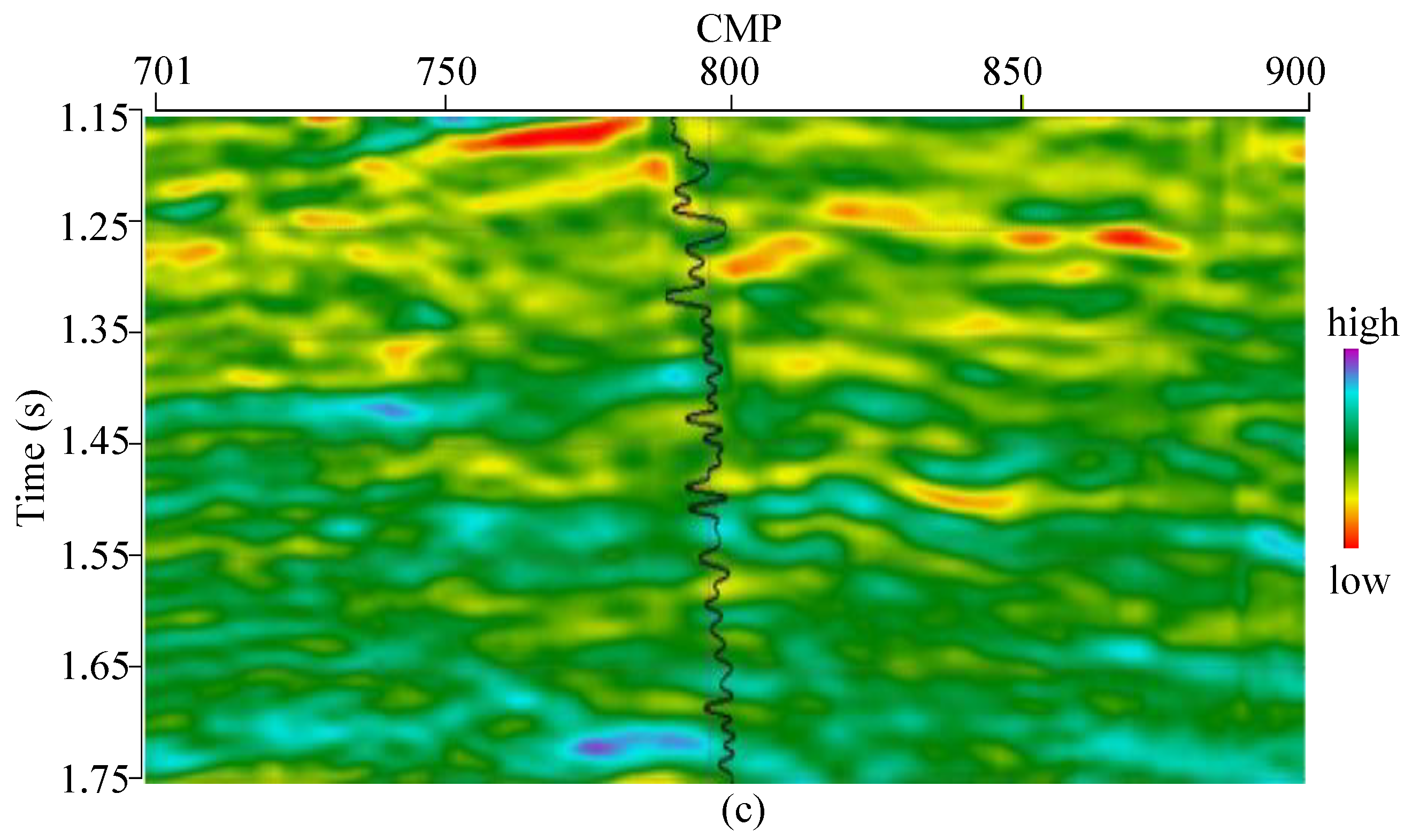
Figure 4 shows the inverted model parameters by L0-AVA inversion, where Figure 4a–c are P-wave velocity, S-wave velocity and density, respectively. In Figure 4, the well log curves across this seismic inline are also overlaid. We can see that the inverted model parameters are well matched with original real seismic data profiles with good structural configurations and stratigraphic lateral distributions.

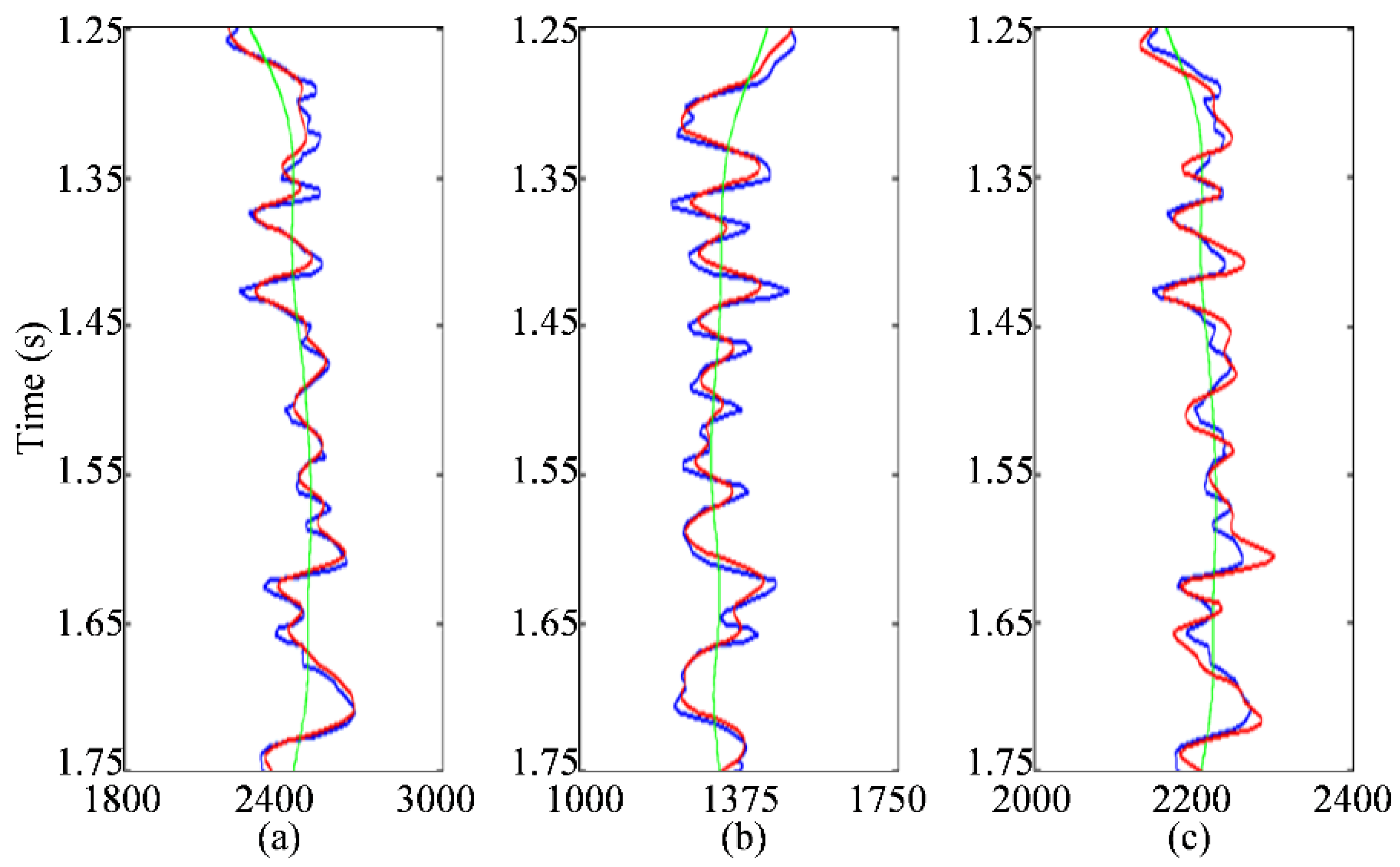
To further display the inversion results, Figure 5 shows a single trace comparison between well log curves and inverted model parameters. The blue curves are well log, the red curves are inverted model parameters and the green curves are the initial model. We can see that the inverted model parameters are also well matched with well log curves.

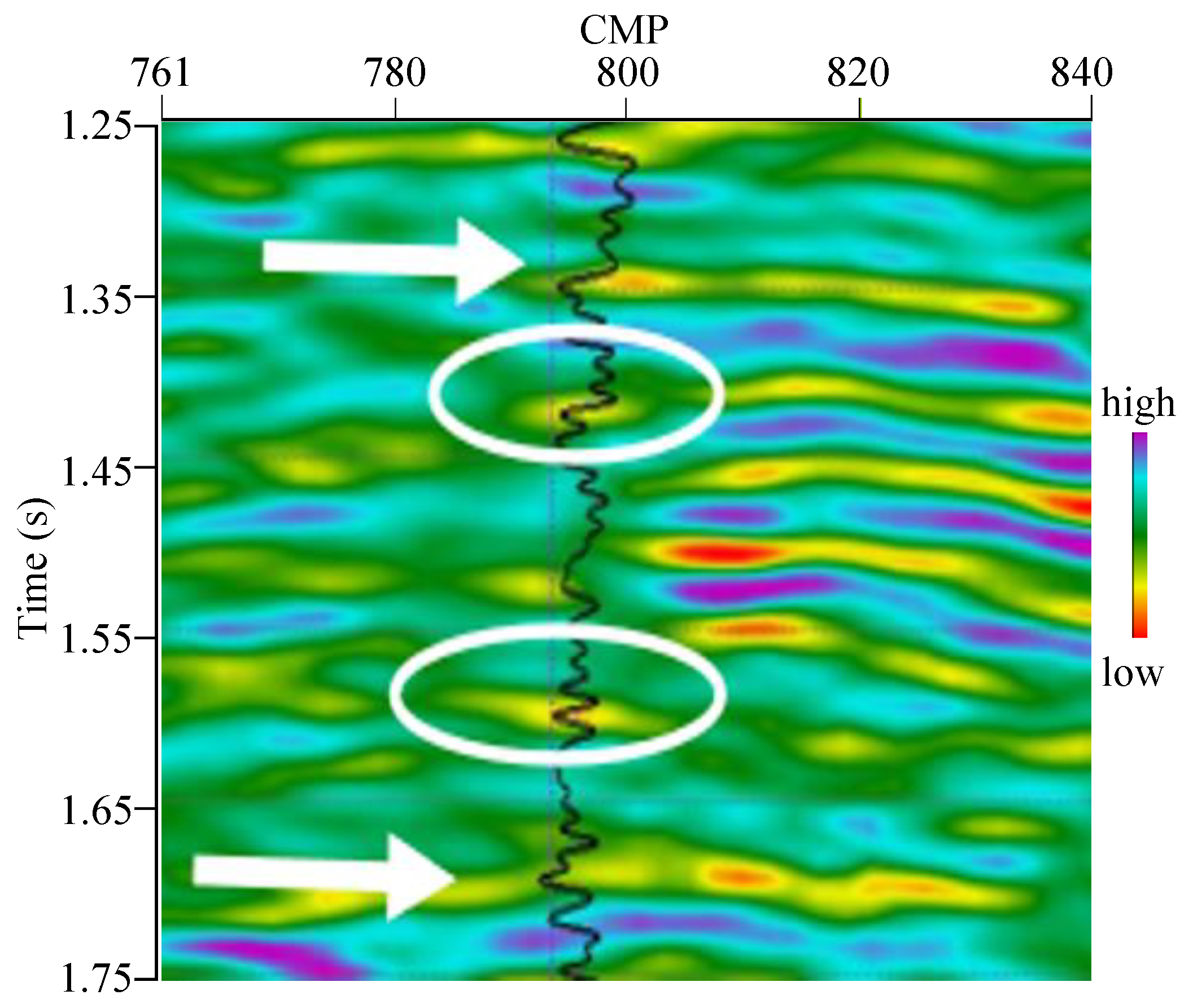
This seismic line is located on the reverse drag anticline structure, which develops faults. It can be seen from the angle stack seismic data profiles that there are many different level faults in this seismic line. The target stratums are fluvial facies deposits, and the lithology changes rapidly. The main oil-producing interval is suited to the upper wall. The locations of white arrows and ellipses shown in the inverted S-wave velocity profiles are oil-bearing sandstone from the interpretation of the well log. Both oil-bearing stratums have lower P-wave velocity, S-wave velocity, and density compared to the surrounding rock. Figure 6 shows the zoomed area of white arrows and ellipses shown in the inverted S-wave velocity profiles to clearly delineate the reservoirs. The reservoir’s outlines are very clear to allow us to distinguish the upper and lower interfaces of target stratums. The clear vertical and spatial variation features of inverted model parameters profiles can be further used in reservoir prediction and description. The results of L0-AVA inversion provide reliable data support for the next work stages in the oil industry.

5. Discussion and Conclusions

AVA inversion is a way to estimate P-wave velocity, S-wave velocity and density from pre-stack seismic data. The distribution of estimated P-wave velocity, S-wave velocity and density are frequently used to mark rock characteristics and help stratigraphic analysis. However, conventional AVA inversion is sensitive to noise in seismic data. In this paper, we merged the two stages in conventional AVA inversion into a single problem to estimate P-wave velocity, S-wave velocity and density directly. The merged inversion method is less sensitive to noise compared to conventional AVA inversion.

To regularize the merged AVA inversion, we adopted the L0-norm-gradient of model parameters. The case of L0-norm regularization is a synthesis formulation, and the case of L0-norm-gradient is an analysis formulation [12]. The difference operator of gradient calculation in the analysis formulation corresponds to the Heaviside synthesis dictionary [12]. Therefore, L0-norm-gradient regularization constrains AVA inversion results with spare representation coefficients on the Heaviside synthesis dictionary. Hence, in AVA inversion, L0-norm-gradient regularization can provide inversion results with blocky features to make formation interfaces and geological edges precise.

From the tests of synthetic seismic data traces, we can conclude that compared to conventional AVA inversion, the inverted model parameters by L0-norm-gradient regularized AVA inversion are better matched with true model parameters and has obvious “blocky” geological characteristics, with only small vibrations at contrast interfaces. The inverted model parameters by L0-norm-gradient regularized AVA inversion are more accurate with higher resolution. From the applications of real seismic lines, we can conclude that the inverted model parameters are well matched with original real seismic data profiles with good structural configurations and stratigraphic lateral distributions. In addition, the inverted model parameters are also well matched with well log curves. The reservoir’s outlines are very clear to allow us to distinguish the upper and lower interfaces of target stratums. The clear vertical and spatial variation features of inverted model parameters profiles can be further used in reservoir prediction and description. The results of L0-norm-gradient regularized AVA inversion provide reliable data support for the next work stages in the oil industry. It is an effective way to estimate P-wave velocity, S-wave velocity and density.