Machine Learning at the Service of Survival Analysis: Predictions Using Time-to-Event Decomposition and Classification Applied to a Decrease of Blood Antibodies against COVID-19

Abstract

The Cox proportional hazard model may predict whether an individual belonging to a given group would likely register an event of interest at a given time. However, the Cox model is limited by relatively strict statistical assumptions. In this study, we propose decomposing the time-to-event variable into “time” and “event” components and using the latter as a target variable for various machine-learning classification algorithms, which are almost assumption-free, unlike the Cox model. While the time component is continuous and is used as one of the covariates, i.e., input variables for various classification algorithms such as logistic regression, naïve Bayes classifiers, decision trees, random forests, and artificial neural networks, the event component is binary and thus may be modeled using these classification algorithms. Moreover, we apply the proposed method to predict a decrease or non-decrease of IgG and IgM blood antibodies against COVID-19 (SARS-CoV-2), respectively, below a laboratory cut-off, for a given individual at a given time point. Using train-test splitting of the COVID-19 dataset ($n=663$ individuals), models for the mentioned algorithms, including the Cox proportional hazard model, are learned and built on the train subsets while tested on the test ones. To increase robustness of the model performance evaluation, models’ predictive accuracies are estimated using 10-fold cross-validation on the split dataset. Even though the time-to-event variable decomposition might ignore the effect of individual data censoring, many algorithms show similar or even higher predictive accuracy compared to the traditional Cox proportional hazard model. In COVID-19 IgG decrease prediction, multivariate logistic regression (of accuracy $0.811$), support vector machines (of accuracy $0.845$), random forests (of accuracy $0.836$), artificial neural networks (of accuracy $0.806$) outperform the Cox proportional hazard model (of accuracy $0.796$), while in COVID-19 IgM antibody decrease prediction, neither Cox regression nor other algorithms perform well (best accuracy is $0.627$ for Cox regression). An accurate prediction of mainly COVID-19 IgG antibody decrease can help the healthcare system manage, with no need for extensive blood testing, to identify individuals, for instance, who could postpone boosting vaccination if new COVID-19 variant incomes or should be flagged as high risk due to low COVID-19 antibodies.

1. Introduction

In survival analysis, the time-to-event variable is usually dependent, i.e., a response variable, and describes whether an individual may expect to experience an event of interest and, if so, when they should do it. If an individual does not experience the event of interest for some reason, we call the individual censored. The event of interest could be whatever defined and detectable event that is not related to censoring [1].

In statistics and survival analysis, the time-to-event variable is commonly treated as a random variable and modeled using traditional approaches, including estimating, both parametric and non-parametric, of a cumulative distribution function and others, namely survival function and hazard function and its moment characteristics. While the survival function depicts a probability that time to an event of interest is greater than a given time constant, i.e., that an individual would survive a certain time, the hazard function is a rate of probability that the event of interest is registered for in an infinitely short time after a given time period of non-registering the event [2].

The above-mentioned approach enables the application of statistical inference on the time-to-event variable and its derivations for one or more groups of individuals. Besides survival functions, comparison between groups of individuals, considering explanatory covariates, the hazard function might be modeled within a regression framework using a Cox proportional hazard model [3].

The Cox proportional hazard model is routinely used for modeling an association between the covariates as independent variables and the hazard function as a dependent variable. However, the Cox model is relatively strictly limited by statistical assumptions [4]. Supposing that there is a categorical independent variable determining which group an individual belongs to, the limiting fact is that proportions of hazard functions for each pair of groups should be constant across all time points; this is why the Cox model is called “proportional” [5,6]. There are several options for how to overcome the violation of non-proportionality of hazard curves, e.g., some covariates in the Cox model may be stratified for different values or groups of individuals that enable the relaxing of the strict assumption that mutual pair hazard curves’ proportions should be equal to one constant [7,8]. Even more, if needed, not only time-invariant covariates but also time-variant explanatory variables could be modified in time-varying models [9], or intervals of time points might be split within time-partitioned models [10]. Various possibilities of the Cox model assumptions’ violation treatment within the large family of Cox non-proportional hazard models suggest that not one of them is an optimal “remedy” for all new assumptions coming from them. The Cox non-proportional hazard models are highly complex, usually require a sufficient amount of data and advanced erudition and experience in their usage, and could bring new assumptions, sometimes even more complex [11]. Besides the Cox models, parametric survival models use log-normal or Weibull baseline hazard function. Although applied to real-world data, these sometimes work better than the Cox regression [12], some others fail, compared to the Cox model [13]. The parametric survival models might suffer an initial choice of the baseline hazard function. In addition, even these models assume the proportionality of hazard functions among individuals or cohorts across time points [14].

In this study, we address the latter issue and propose an alternative to the Cox proportional hazard model that is almost assumption-free. We introduce a principle of time-to-event variable decomposition into two components; first, a time component that is continuous and is used as an explanatory covariate in a machine-learning classification model, and second, an event component that is binary and could be predicted using various classifiers in the classification models, containing, besides others, the time component as an input covariate. Finally, once a classification model is learned and built, then, for a given combination of values of explanatory covariates, including a time point since the time component is one of the covariates, we may predict whether an event of interest is likely to happen for the given covariates’ values combination. The same prediction might be made using the Cox proportional hazard model—the model estimates the posterior distribution of hazard function, which enables obtaining the point estimate of the probability that an individual with given covariates’ values combination would likely experience the event of interest. If the probability is greater than or equal to a defined threshold, we obtain qualitatively the same prediction as using our proposed method. This opens room for comparison of predictive accuracy between our introduced method based on time-to-event variable decomposition and the Cox proportional hazard model. While the Cox proportional hazard model considers the non-experiencing event of interest within a given time scope as the censoring, machine-learning classifiers understand the experiencing and non-experiencing event of interest as two potentially equal states and, thus, might sideline the censoring in this manner. However, if we prefer the prediction paradigm rather than the inference one, censoring as a kind of incomplete information might be sidelined as far as the prediction work with high enough performance.

The first ideas on time-to-event variable decomposition came from the eighties when Blackstone et al. tried to decompose the time-to-event variable into consecutive phases and model a constant hazard function for each phase [15]. The approach was revisited during the last several years by [16,17] since time-varying and time-partitioning models became popular. However, papers dealing with the combination of time-to-event variable decomposition and machine-learning predictions on the components seem to be rare; some initial experiments come from [18], where authors tried to predict survival in patients with stomach cancer.

The machine-learning classification models might differ in their predictive accuracy; however, regardless of the built classifiers, these are usually assumption-free or assumption-almost-free [19]. We consider several classification algorithms in the study—multivariate logistic regression, naïve Bayes classifier, decision trees, random forests, and artificial neural networks.

To obtain an idea of how the proposed methodology works on real data, we apply the time-to-event decomposition and ongoing prediction on a dataset of COVID-19 patients that includes, besides others, a variable depicting whether, and if so, when an individual experienced a decrease of their COVID-19 antibody blood level below a laboratory cut-off. Some of the individuals in the dataset did experience the antibody blood level decrease; the other ones did not. Thus, the variable is appropriate to be treated as a time-to-event one. COVID-19 is an infectious disease caused by the virus SARS-CoV-2 that started with the first clinically manifesting cases at the end of the year 2019 and quickly spread worldwide [20]. Thus, from early 2020 up to the present, there has been more or less a severe long-term pandemic in many regions all around the world [21,22]. Individuals’ COVID-19 blood antibodies, particularly IgG antibodies that are more COVID-19-specific, protect them from COVID-19 manifesting disease [23]. Therefore, if we predict their decrease below laboratory cut-off accurately enough, we can, for instance, quickly, and with no need for extensive or expensive blood testing, preselect which individuals should undergo boosting vaccination first if a new COVID-19 variant would income.

Thus, in this article, we address the following research gap. First, we investigate how possible it is to predict a decrease of antibodies against COVID-19 in time using various individuals’ covariates and a Cox proportional hazard model. Moreover, we introduce a novel method for predicting an event of interest’s occurrence in time using time-to-event decomposition, where the event component is classified using machine-learning classification algorithms. In contrast, the time component is used as one of the covariates. Finally, we compare the predictive performance of Cox regression and our proposed method using predictive accuracy and other metrics.

The paper proceeds as follows. Firstly, in Section 2, we introduce and explain ideas of our proposed methodology, mostly the logic and principles of the time-to-event decomposition. Then, we illustrate the principles, assumptions, and limitations of the Cox proportional hazard model. In addition, we describe how the prediction of an event of interest’s occurrence could be made using the Cox model. Then, we depict all machine-learning classification algorithms’ principles. Next, in Section 3, we show the numerical results we have obtained so far and, in particular, compare predictions based on the Cox proportional hazard model with other predictions, using classifiers and time-to-event decomposition. Finally, in Section 4, we discuss the results, explain them, and last but not least, we highlight important findings in Section 5.

2. Methodology and Data

A description of the fundamentals of survival variables’ characteristics, the Cox proportional hazard model, the proposed methodology, and the dataset we used for algorithms’ predictive performance, respectively, follow.

2.1. Fundamentals of Survival Variables’ Characteristics

Let us assume that a random variable T is the survival time, i.e., a length of time an individual does not experience an event of interest [24]. Firstly, let us define survival function $S\left(t\right)$ as a probability that survival time is greater than some time constant t, so

$$S\left(t\right)=P(T>t)=P(T\ge t)-P(T=t)=P(T\ge t)-0=P(T\ge t).$$

(1)

Let cumulative distribution function $F\left(t\right)$ be a probability that survival time T would not be greater than time constant t; then, density function $f\left(t\right)$ is a derivative of $F\left(t\right)$ with respect to t, so

$$\begin{array}{cc}\hfill f\left(t\right)& =\frac{\mathrm{d}F\left(t\right)}{\mathrm{d}t}=\frac{\mathrm{d}P(T\le t)}{\mathrm{d}t}=\frac{\mathrm{d}(1-P(T>t\left)\right)}{\mathrm{d}t}=\frac{\mathrm{d}1}{\mathrm{d}t}-\frac{\mathrm{d}P(T>t))}{\mathrm{d}t}=\hfill \\ \hfill & =0-\frac{\mathrm{d}P(T>t))}{\mathrm{d}t}=-\frac{\mathrm{d}P(T>t)}{\mathrm{d}t}\stackrel{\left(1\right)}{=}-\frac{\mathrm{d}S\left(t\right)}{\mathrm{d}t}\hfill \end{array}$$

(2)

and also

$$f\left(t\right)=-\frac{\mathrm{d}P(T>t)}{\mathrm{d}t}=\underset{\Delta t\to 0}{lim}\frac{P(t+\Delta t>T\ge t)}{\Delta t}.$$

(3)

The hazard function, $\lambda \left(t\right)$, is an instantaneous probability that an individual experiences the event of interest in an indefinitely short time interval $\langle t,t+\Delta t)$ once they survive through time t up to the beginning of the interval $\langle t,t+\Delta t)$, so

$$\begin{array}{cc}\hfill \lambda \left(t\right)& =\underset{\Delta t\to 0}{lim}\frac{P\left(T\in \langle t,t+\Delta t)\mid T\ge t\right)}{\Delta t}=\underset{\Delta t\to 0}{lim}\frac{P(t+\Delta t>T\ge t\mid T\ge t)}{\Delta t}=\hfill \\ \hfill & =\underset{\Delta t\to 0}{lim}\frac{P(t+\Delta t>T\ge t\wedge T\ge t)}{\Delta t·P(T\ge t)}=\underset{\Delta t\to 0}{lim}\frac{P(t+\Delta t>T\ge t)}{\Delta t·P(T\ge t)}\stackrel{\left(1\right)}{=}\hfill \\ \hfill & \stackrel{\left(1\right)}{=}\frac{1}{S\left(t\right)}\underset{\Delta t\to 0}{lim}\frac{P(t+\Delta t>T\ge t)}{\Delta t}\stackrel{\left(3\right)}{=}\frac{1}{S\left(t\right)}f\left(t\right)\stackrel{\left(2\right)}{=}-\frac{1}{S\left(t\right)}\frac{\mathrm{d}S\left(t\right)}{\mathrm{d}t}=-\frac{S^{\prime }\left(t\right)}{S\left(t\right)}.\hfill \end{array}$$

(4)

Since hazard function $\lambda \left(t\right)={lim}_{\Delta t\to 0}\frac{P\left(T\in \langle t,t+\Delta t)\mid T\ge t\right)}{\Delta t}$ describes an instantaneous probability of an event of interest experiencing just after a specific time t, we could estimate cumulative hazard function $\Lambda \left(t\right)$ as an accumulation of the hazard of the event of interest over time until constant t, having estimates $\widehat{\lambda }\left(t_j\right)$, based e.g., on observed data, for each time point from the beginning to the end of the observed period. That being said,

$$\Lambda \left(t\right)\approx \sum _{\forall t_j:t_j\le t}\widehat{\lambda }\left(t_j\right),$$

or more precisely as

$$\Lambda \left(t\right)={\int }_0^t\lambda \left(\tau \right)\mathrm{d}\tau ,$$

(5)

which may help us to derive a relationship between the survival function and hazard function as follows:

$$\Lambda \left(t\right)={\int }_0^t\lambda \left(\tau \right)\mathrm{d}\tau \stackrel{\left(4\right)}{=}{\int }_0^t-\frac{S^{\prime }\left(\tau \right)}{S\left(\tau \right)}\mathrm{d}\tau ={\left[-logS\left(\tau \right)\right]}_0^t,$$

and since $S\left(0\right)=P(T>0)=P(T\ge 0)=1$, we obtain

$$\begin{array}{cc}\hfill \Lambda \left(t\right)& ={\left[-logS\left(\tau \right)\right]}_0^t=-logS\left(t\right)-(-logS\left(0\right))=\hfill \\ \hfill & =-logS\left(t\right)+log1=-logS\left(t\right)+0=\hfill \\ \hfill & =-logS\left(t\right).\hfill \end{array}$$

(6)

Finally, by exponentiation of Formula (6), we obtain a direct relationship between the survival function and cumulative hazard function,

$$S\left(t\right)=e^{-\Lambda \left(t\right)},$$

(7)

which enables us to predict survival probability for a given time point, based on the Cox proportional hazard model.

2.2. Principles, Assumptions and Limitations of Cox Proportional Hazard Model

The Cox proportional hazard model is frequently used for regression modeling of an association between a hazard function for an event of interest as a dependent variable and multiple independent variables, also called covariates.

Sir Cox [3] suggested to model the hazard function $\lambda \left(t\right)$ in relation to other $k\in \mathbb{N}$ covariates ${\mathit{X}}_i={(X_{i,1},X_{i,2},\dots ,X_{i,k})}^T$ for individual or group i in the following way:

$$log\lambda \left(t\right)=log{\lambda }_0\left(t\right)+{\mathit{\beta }}^T{\mathit{x}}_i,$$

(8)

where ${\lambda }_0\left(t\right)$ is the baseline hazard function, i.e., the hazard function when each of the covariates is equal to zero; $\mathit{\beta }={({\beta }_0,{\beta }_1,{\beta }_2,\dots ,{\beta }_k)}^T$ is a vector of linear coefficients, each matched to an appropriate covariate, and ${\mathit{x}}_i=(1,x_{i,1},x_{i,2},\dots ,x_{i,k})$ is a vector of covariates’ values for individual or group i. The linear coefficients $\mathit{\beta }={({\beta }_0,{\beta }_1,{\beta }_2,\dots ,{\beta }_k)}^T$ in the Cox model following Formula (8) can be estimated using the partial maximum likelihood approach [25,26].

By exponentiation Formula (8), we obtain another form of the Cox model,

$$\lambda \left(t\right)=e^{log{\lambda }_0\left(t\right)+{\mathit{\beta }}^T{\mathit{x}}_i}=e^{log{\lambda }_0\left(t\right)}·e^{{\mathit{\beta }}^T{\mathit{x}}_i}={\lambda }_0\left(t\right)·e^{{\mathit{\beta }}^T{\mathit{x}}_i}.$$

(9)

Considering the Cox model following Formula (9) for two groups with indices r and s,

$$\begin{array}{cc}\hfill \lambda (t\mid {\mathit{x}}_r)& ={\lambda }_0\left(t\right)·e^{{\mathit{\beta }}^T{\mathit{x}}_r}\hfill \\ \hfill \lambda (t\mid {\mathit{x}}_s)& ={\lambda }_0\left(t\right)·e^{{\mathit{\beta }}^T{\mathit{x}}_s},\hfill \end{array}$$

we could take a proportion of left-hand and right-hand sides of the equations, obtaining

$$\frac{\lambda (t\mid {\mathit{x}}_r)}{\lambda (t\mid {\mathit{x}}_s)}=\frac{{\lambda }_0\left(t\right)·e^{{\mathit{\beta }}^T{\mathit{x}}_r}}{{\lambda }_0\left(t\right)·e^{{\mathit{\beta }}^T{\mathit{x}}_s}}=\frac{e^{{\mathit{\beta }}^T{\mathit{x}}_r}}{e^{{\mathit{\beta }}^T{\mathit{x}}_s}}.$$

(10)

Assuming the model’s coefficient following Formula (8) or Formula (9) are estimated taking into account, for all individuals or groups, ${\mathit{x}}_i=(x_{i,1},x_{i,2},\dots ,x_{i,k})$ for $\forall i\in \{1,2,\dots \}$, i.e.,

$${\mathit{\beta }}^T{\mathit{x}}_r=\mathrm{const}.\mathrm{and}{\mathit{\beta }}^T{\mathit{x}}_s=\mathrm{const}.,$$

we may derive—using Formula (10)—that the proportion

$$\frac{\lambda (t\mid {\mathit{x}}_r)}{\lambda (t\mid {\mathit{x}}_s)}=\frac{e^{{\mathit{\beta }}^T{\mathit{x}}_r}}{e^{{\mathit{\beta }}^T{\mathit{x}}_s}}=\mathrm{const}.$$

of hazard functions for two any groups $r,s\in \{1,2,\dots \}$ is supposed to be constant. This is why the Cox model is called the Cox proportional hazard model, and the constant proportion of the hazard functions across all time points for any two groups is one of its statistical assumptions. Moreover, if the hazard functions’ ratio should be constant, then also survival functions’ ratio should be constant, as we may see using Formulas (5) and (7),

$$\frac{\lambda (t\mid {\mathit{x}}_r)}{\lambda (t\mid {\mathit{x}}_s)}=\frac{\int \lambda (t\mid {\mathit{x}}_r)\mathrm{d}t}{\int \lambda (t\mid {\mathit{x}}_s)\mathrm{d}t}=\frac{e^{-\int \lambda (t\mid {\mathit{x}}_r)\mathrm{d}t}}{e^{-\int \lambda (t\mid {\mathit{x}}_s)\mathrm{d}t}}=\frac{e^{-\Lambda (t\mid {\mathit{x}}_r)}}{e^{-\Lambda (t\mid {\mathit{x}}_s)}}=\frac{S(t\mid {\mathit{x}}_r)}{S(t\mid {\mathit{x}}_s)}=\mathrm{const}.$$

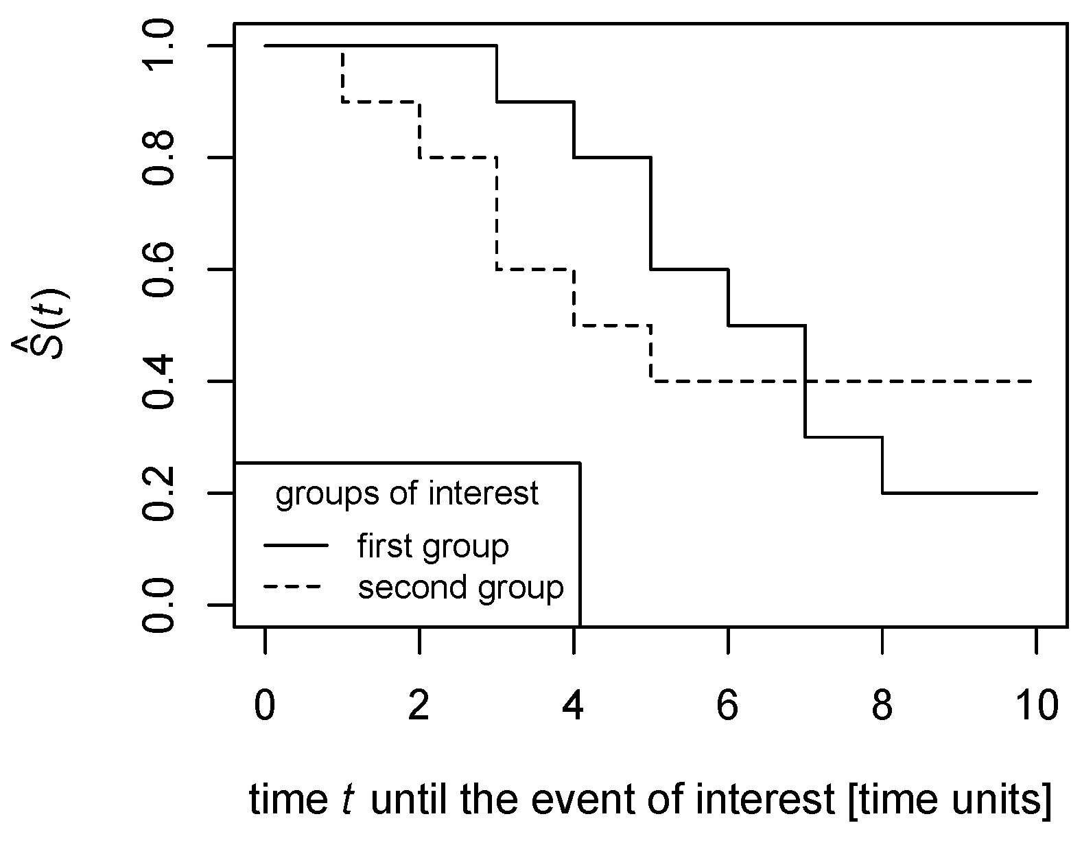
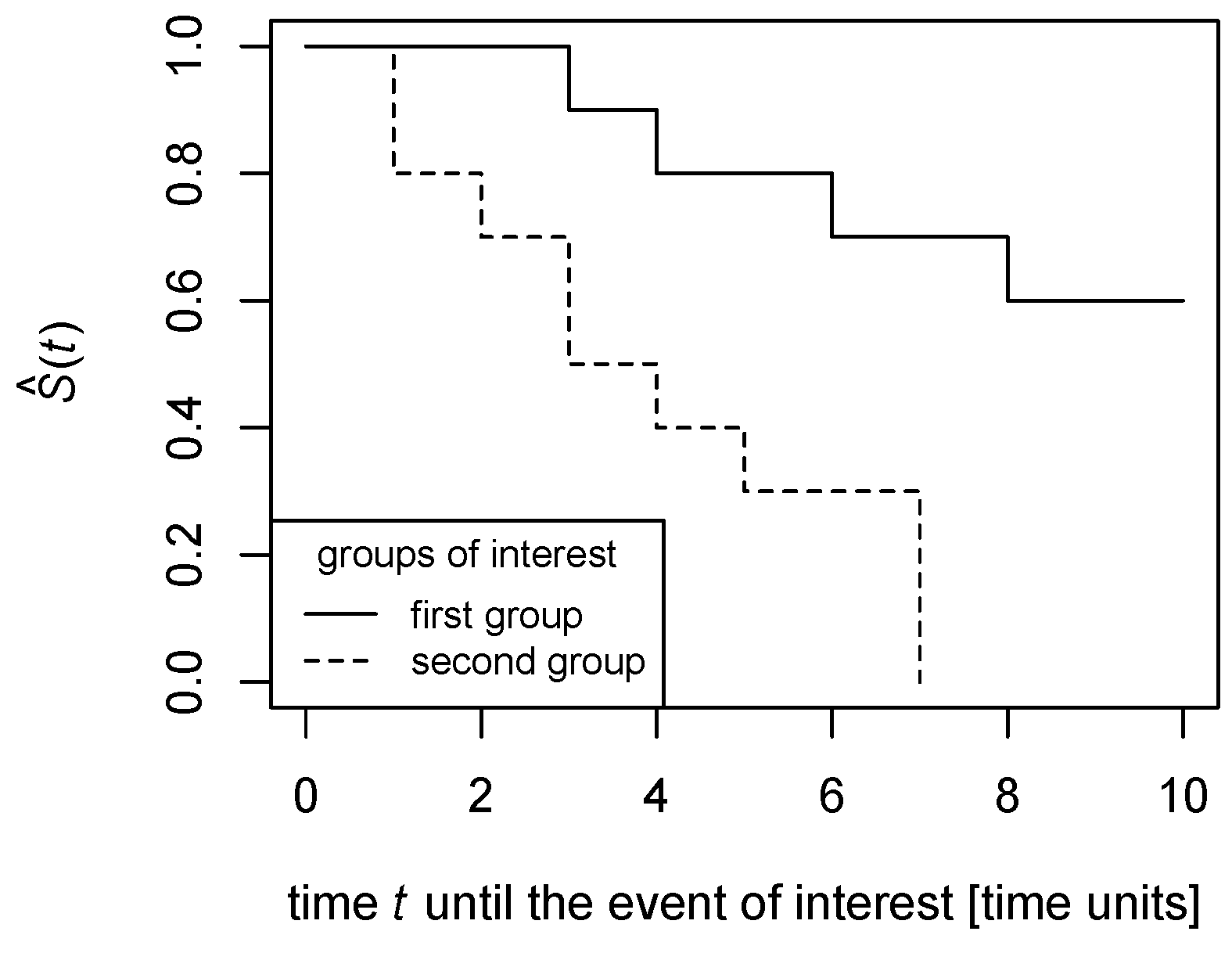
However, real-world data often violate this assumption in practice, as Figure 1 and Figure 2 illustrate.

In Figure 1, the survival functions are estimated in a non-parametric way as polygonal chains cross each other; this means that, while the proportion of the survival function for the solid line to the survival function for the dashed line is greater than 1 till the time point of the crossing, it becomes lower than 1 after the crossing. Thus, the survival functions’ proportion could not be constant across all time points.

Similarly, in Figure 2, the proportion of the survival function for the solid line to the survival function for the dashed line is finite until the time point the dashed line drops to zero, then the proportion becomes infinite. Therefore, the survival functions’ ratio could not be constant across all time points.

Considering the Cox model from Formula (8) and using Formula (7), we can predict whether an event of interest is likely to be experienced by an individual from a given group at a given time point. Survival function, i.e., a probability that an individual does not experience the event of interest before time t, if ever, is

$$S\left(t\right)=P(T>t)=e^{-\Lambda \left(t\right)}=e^{-{\int }_0^t\lambda \left(t\right)\mathrm{d}t}=e^{-{\int }_0^t{\lambda }_0\left(t\right)·e^{{\mathit{\beta }}^T{\mathit{x}}_i}\mathrm{d}t},$$

and using estimates coming from the Cox model following Formula (8),

$$\widehat{S}\left(t\right)=\widehat{P}(T>t)=e^{-\widehat{\Lambda }\left(t\right)}=e^{-{\int }_0^t\widehat{\lambda }\left(t\right)\mathrm{d}t}=e^{-{\int }_0^t{\widehat{\lambda }}_0\left(t\right)·e^{{\widehat{\mathit{\beta }}}^T{\mathit{x}}_i}\mathrm{d}t}.$$

(11)

2.3. Principles of Proposed Time-to-Event Variable Decomposition and Prediction

The Cox proportional hazard model, following the Formula (8) or Formula (9), estimates the posterior hazard function using covariates $\mathit{X}={(X_1,X_2,\dots ,X_k)}^T$, i.e., it models the posterior probability of an event of interest’s occurrence in time [27].

Let us mark the time to the event of interest for any individual or group as a random variable T, and the occurrence or non-occurrence of the event of interest for any individual or group as a random variable Y. Obviously, $T_i\ge 0$, and $Y_i\in \{c_1,c_2\}$, or generally $Y_i\in \left\{c_{\ell }\right\}$ considering $\ell \in \{1,2\}$, for individual or group i, where $c_1$ stands for the event of interest occurrence before time t and $c_2$ stands for the event of interest non-occurrence before time t, respectively.

With respect to the task refining above, the Cox proportional hazard model uses covariates $\mathit{X}={(X_1,X_2,\dots ,X_k)}^T$ and their values ${\mathit{x}}_i={(x_{i,1},x_{i,2},\dots ,x_{i,k})}^T$ for estimation, a pair $[T_i,Y_i]$ for individual or group i, i.e., how likely individual or group i would experience ($Y_i=c_1$), or would not experience ($Y_i=c_2$) the event of interest until time $T_i=t$.

Inspecting Formula (11), we may see that the time $T=t$ is a parameter of the survival estimate $\widehat{S}\left(t\right)$. However, the event of interest’s occurrence or non-occurrence $Y\in \{c_1,c_2\}$ requires another derivation. Once the Cox model is built, the coefficients $\mathit{\beta }={({\beta }_0,{\beta }_1,{\beta }_2,\dots ,{\beta }_k)}^T$ are estimated using all dataset rows ${\mathit{x}}_i=(1,x_{i,1},x_{i,2},\dots ,x_{i,k})$ for $\forall i\in \{1,2,\dots \}$, the survival $\widehat{S}\left(t\right)$ might be estimated using Formula (11). Since $S\left(t\right)=P(T>t)$, we may expect that the event of interest does probably not occur before time t if $\widehat{S}\left(t\right)=\widehat{P}(T>t)$ is high enough. Let us suppose the event of interest is likely not to happen, $Y=c_2$, before time t, if ever does, whenever $\widehat{S}\left(t\right)$ is greater than or equal to a given threshold $p_{\mathrm{threshold}}$; otherwise, the event of interest does probably occur, $Y=c_1$, before time t. Thus,

$$\widehat{Y}=\left\{\begin{array}{cc}{c}_1, \mathrm{i}.\mathrm{e}., \mathrm{the}\mathrm{event} \mathrm{of} \mathrm{interest} \mathrm{does} \mathrm{occur} \mathrm{before} \mathrm{time} t\hfill & \widehat{S}\left(t\right)<p_{\mathrm{threshold}}\hfill \\ c_2, \mathrm{i}.\mathrm{e}., \mathrm{the}\mathrm{event} \mathrm{of} \mathrm{interest} \mathrm{does} \mathrm{not} \mathrm{occur} \mathrm{before} \mathrm{time} t\hfill & \widehat{S}\left(t\right)\ge p_{\mathrm{threshold}}\hfill \end{array}\right.$$

(12)

A natural choice for the threshold seems to be $p_{\mathrm{threshold}}=\frac{1}{2}$, but may be grid-searched and adjusted, e.g., to maximize the Cox model’s predictive accuracy.

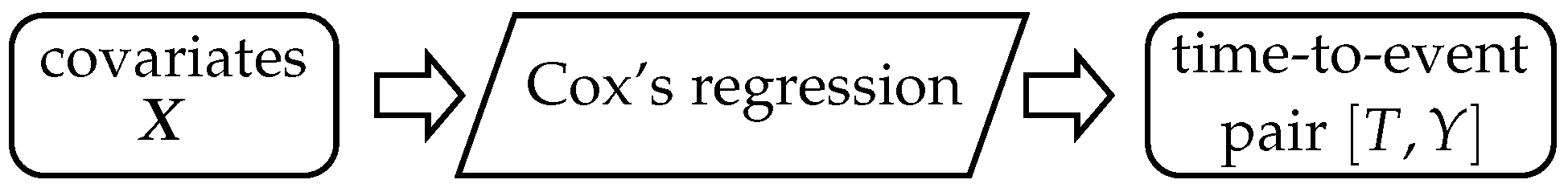
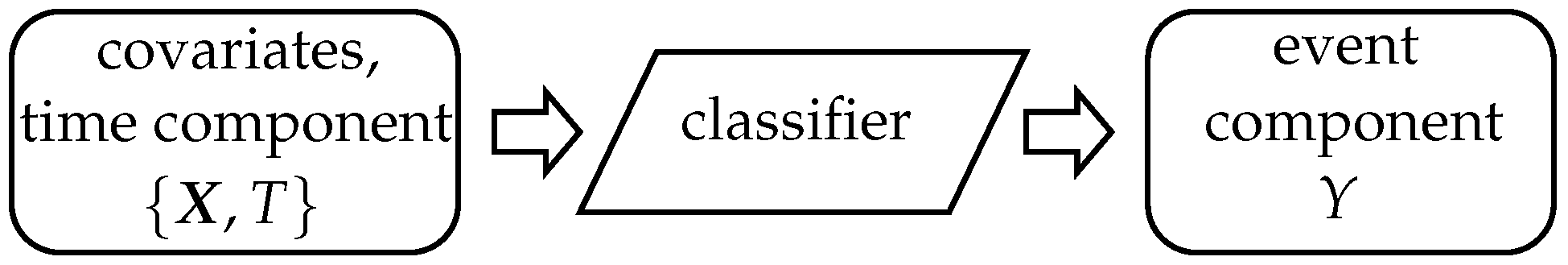
Schematically, the logic of the Cox model is in Figure 3. Covariates $\mathit{X}={(X_1,X_2,\dots ,X_k)}^T$ are on input and make the Cox model’s estimation possible. Once the Cox model is built, we could predict the event of interest occurrence $Y\in \{c_1,c_2\}$ in time $T=t$ using Formulas (11) and (12). Thus, on the input of the Cox model, there are k covariates $\{X_1,X_2,\dots ,X_k\}$, and on output, there is the time-to-event pair variable $[T,Y]$.

We refine the task of time-to-event prediction the following way. Firstly, we decompose the time-to-event variable into time component T and event component Y. The time component T is continuous and is used as another covariate on input for a machine-learning classification model or, shortly, a classifier. The machine-learning classification model predicts the event component Y on output, i.e., whether the event of interest likely occurs ($Y=c_1$) or not ($Y=c_2$) before time t, using values of covariates ${(X_1,X_2,\dots ,X_k)}^T={(x_1,x_2,\dots ,x_k)}^T$ and a value of time $T=t$ as explanatory variables. Thus, on input of the classifier, there are $k+1$ covariates $\{X_1,X_2,\dots ,X_k,T\}$, and on output, there is the event component Y, as the scheme in Figure 4 illustrates.

As a classification algorithm, various approaches, such as multivariate logistic regression, naïve Bayes classifiers, decision trees, random forests, or artificial neural networks, might be chosen, e.g., to maximize the model’s predictive accuracy.

2.4. Machine-Learning Classification Algorithms

Following the logic of time-to-event variable decomposition and classification-based prediction of an event of interest’s occurrence as demonstrated in the scheme in Figure 4, we describe principles of selected classifying algorithms used for the model building and predicting a COVID-19 antibody blood level decrease below laboratory cut-off.

In general, all classifiers listed below employ covariates $\mathit{X}={(X_1,X_2,\dots ,X_k,T)}^T$ on input and classify into two classes, either $c_1$, or $c_2$ of a target variable Y, i.e., an event of interest occurrence or non-occurrence before time t.

2.4.1. Multivariate Logistic Regression

Multivariate logistic regression classifies into one of the classes $\{c_1,c_2\}$, i.e., an event of interest occurrence and non-occurrence, of the target variable Y using $k+1$ covariates $X_1,X_2,\dots ,X_k,T$. A formula of the multivariate logistic regression [28] follows for individual i a form of

$$log\frac{P(Y_i=c_l\mid {\mathit{x}}_i,t_i)}{1-P(Y_i=c_1\mid {\mathit{x}}_i,t_i)}={\beta }_0+\sum _{j=1}^k{\beta }_j{x}_i+{\beta }_{k+1}{t}_i+{\epsilon }_i,$$

where ${\beta }_0$ is an intercept, ${\beta }_j$ are linear coefficients each matched to covariate $X_j$ for $j\in \{1,2,\dots ,k\}$, ${\beta }_{k+1}$ is a linear coefficient matched to time component T, vector ${\mathit{x}}_i=(x_{i,1},x_{i,2},\dots ,x_{i,k})$ contains values of appropriate covariates $X_j$ for individual i, where $j\in \{1,2,\dots ,k\}$, and ${\epsilon }_i$ is a residual for individual i.

The linear coefficients are estimated numerically using maximal likelihood [29]. Individual i’s value of variable Y is classified using a maximum-a-posteriori principle into final class $c_{\ell }^{*}$ so that

$$c_{\ell }^{*}=arg\underset{\ell \in \{1,2\}}{max}\left\{P(Y=c_{\ell }\mid {\mathit{x}}_i,t_i)\right\}.$$

2.4.2. Naïve Bayes Classifier

Naïve Bayes classifier also predicts the most likely class $c_{\ell }^{*}\in \{c_1,c_2\}$ of the target variable Y, where $c_1$ stands for the event of interest occurrence and $c_2$ for the event of interest non-occurrence, respectively [30]. Once we apply Bayes theorem, we obtain

$$P(Y_i=c_{\ell }\mid {\mathit{x}}_i,t_i)=\frac{P({\mathit{x}}_i,t_i\mid Y_i=c_{\ell })P(Y_i=c_{\ell })}{P({\mathit{x}}_i,t_i)}.$$

(13)

Assuming we have a given dataset, i.e., a matrix containing n vectors such as ${\mathit{x}}_i=(x_{i,1},x_{i,2},\dots ,x_{i,k},t_i)$ for $\forall i\in \{1,2,\dots ,n\}$, the probabilities $P(Y_i=c_{\ell })$ and $P({\mathit{x}}_i,t_i)$ are constant, since

$$\widehat{P}(Y_i=c_{\ell })=\frac{\# \mathrm{of} \mathrm{rows} \mathrm{where} Y_i=c_{\ell }}{n}$$

(14)

and

$$\widehat{P}({\mathit{x}}_i,t_i)=\frac{\# \mathrm{of} \mathrm{rows} \mathrm{where} {\mathit{X}}_i={\mathit{x}}_i \mathrm{and} T_i=t_i}{n}.$$

(15)

Moreover, if the dataset is well balanced, then for $\forall \ell \in \{1,2\}$ $\widehat{P}(Y_i=c_{\ell })=\frac{1}{2}$ and for $\forall p,q\in \{1,2,\dots ,n\}$ is $\widehat{P}({\mathit{x}}_p,t_p)=\widehat{P}({\mathit{x}}_q,t_q)$. Thus, we may write for $\forall \ell \in \{1,2\}$ and for $\forall i\in \{1,2,\dots ,n\}$

$$\frac{\widehat{P}(Y_i=c_{\ell })}{\widehat{P}({\mathit{x}}_i,t_i)}=\kappa =\mathrm{const}.$$

(16)

Thus, using Formulas (14)–(16), we might rewrite Formula (13) as follows:

$$\begin{array}{cc}\hfill P(Y_i=c_{\ell }\mid {\mathit{x}}_i,t_i)& =\frac{P({\mathit{x}}_i,t_i\mid Y_i=c_{\ell })P(Y_i=c_{\ell })}{P({\mathit{x}}_i,t_i)}=\hfill \\ \hfill & =P({\mathit{x}}_i,t_i\mid Y_i=c_{\ell })\underset{=\kappa }{\underbrace{\frac{P(Y_i=c_{\ell })}{P({\mathit{x}}_i,t_i)}}}=\hfill \\ \hfill & =P({\mathit{x}}_i,t_i\mid Y_i=c_{\ell })·\kappa \propto \hfill \\ \hfill & \propto P({\mathit{x}}_i,t_i\mid Y_i=c_{\ell })\hfill \end{array}$$

(17)

Assuming mutual independence of covariates $X_1,X_2,\dots ,X_k,T$, we improve Formula (17) as

$$\begin{array}{cc}\hfill P(Y_i=c_{\ell }\mid {\mathit{x}}_i,t_i)& \propto P({\mathit{x}}_i,t_i\mid Y_i=c_{\ell })\propto \hfill \\ \hfill & \propto P(X_{i,1}=x_{i,1}\wedge X_{i,2}=x_{i,2}\wedge \cdots \wedge X_{i,k}=x_{i,k}\wedge T_i=t_i\mid Y_i=c_{\ell })\propto \hfill \\ \hfill & \propto \prod _{j=1}^{k}P(X_{i,j}=x_{i,j}\mid Y_i=c_{\ell })·P(T_i=t_i\mid Y_i=c_{\ell }),\hfill \end{array}$$

and individual i’s value of variable Y is classified into final class $c_{\ell }^{*}\in \{c_1,c_2\}$, using the maximum-a-posteriori principle, so

$$c_{\ell }^{*}=arg\underset{\ell \in \{1,2\}}{max}\left\{\prod _{j=1}^{k}P(X_{i,j}=x_{i,j}\mid Y_i=c_{\ell })·P(T_i=t_i\mid Y_i=c_{\ell })\right\}.$$

The probabilities $P(X_{i,j}=x_{i,j}\mid Y_i=c_{\ell })$ and $P(T_i=t_i\mid Y_i=c_{\ell })$ for categorical covariates could be estimated as

$$\widehat{P}(X_{i,j}=x_{i,j}\mid Y_i=c_{\ell })=\frac{\# \mathrm{of} \mathrm{rows} \mathrm{where} {\mathit{X}}_{i,j}={\mathit{x}}_{i,j} \mathrm{and} Y_i=c_{\ell }}{\# \mathrm{of} \mathrm{rows} \mathrm{where} Y_i=c_{\ell }}$$

and

$$\widehat{P}(T_i=t_i\mid Y_i=c_{\ell })=\frac{\# \mathrm{of} \mathrm{rows} \mathrm{where} T_i=t_i \mathrm{and} Y_i=c_{\ell }}{\# \mathrm{of} \mathrm{rows} \mathrm{where} Y_i=c_{\ell }},$$

for continuous variables, $\widehat{P}(X_{i,j}=x_{i,j}\mid Y_i=c_{\ell })$ and $\widehat{P}(T_i=t_i\mid Y_i=c_{\ell })$ are estimated [31] using conditional normal cumulative distribution function $\widehat{P}(X_{i,j}=x_{i,j}\mid Y_i=c_{\ell })=\Phi (X_{i,j}=x_{i,j}\pm ϵ\mid Y_i=c_{\ell })$ and $\widehat{P}(T_i=t_i\mid Y_i=c_{\ell })=\Phi (T_i=t_i\pm ϵ\mid Y_i=c_{\ell })$, both for small $ϵ>0$.

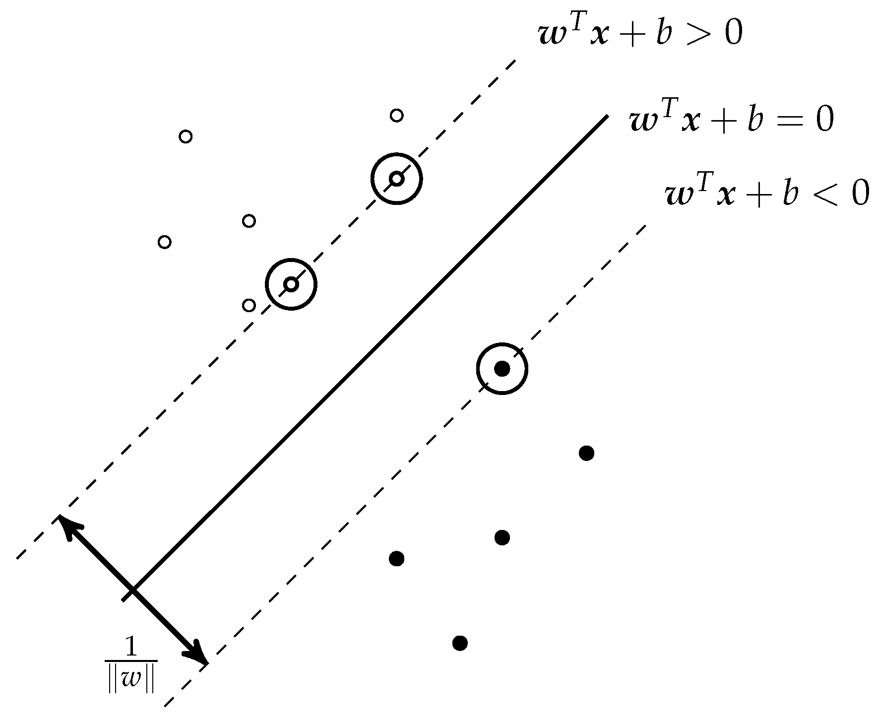
2.4.3. Support Vector Machines

Support vector machines natively split the space of all covariates $X_1\times X_2\times \cdots \times X_k\times T$ into two subspaces by a hyperplane that maximizes the margins between the hyperplane and the points from both subspaces that are the closest to the hyperplane [32]; see Figure 5.

More technically, assuming we have vectors such as ${\mathit{x}}_i={(x_{i,1},x_{i,2},\dots ,x_{i,k},t_i)}^T$, i.e., in other words, these vectors are points in $(k+1)$-dimensional space with coordinates $[x_{i,1},x_{i,2},\dots ,x_{i,k},t_i]$, that belongs either to class $Y=c_1$, or to class $Y=c_2$, any hyperplane in the given universe follows a form of

$${\mathit{w}}^T{\mathit{x}}_i-b,$$

where $\mathit{w}$ is a vector orthonormal, or at least orthogonal to the hyperplane, and b is a tolerated margin’s width, i.e., a user’s hyperparameter, so that $\frac{b}{\parallel \mathit{w}\parallel }$ is the offset of the hyperplane from the universe system of coordinates’ origin along the normal vector $\mathit{w}$.

The splitting hyperplane follows an equation ${\mathit{w}}^T{\mathit{x}}_i-b=0$. For all points that belong to class $Y=c_1$ (and are “above” the splitting hyperplane), we suppose to find a boundary hyperplane that is parallel to the splitting hyperplane, so it should have an equation ${\mathit{w}}^T{\mathit{x}}_i-b>0$. Similarly, all remaining points of class $Y=c_2$ should be on or “below” a boundary hyperplane with equation ${\mathit{w}}^T{\mathit{x}}_i-b<0$. If points of class $Y=c_1$ are “above” and points of class $Y=c_2$ are “below” the splitting hyperplane does not matter much and is addressed by $\delta \in \{-1,+1\}$ term in other equations. Assuming linear separability of the points from different classes and formally assigning $Y=c_1\equiv +1$ and $Y=c_2\equiv -1$, the distance between these two boundary hyperplanes is equal to $\frac{2}{\parallel \mathit{w}\parallel }$ and should be as large as possible, so the searching for max-margin splitting hyperplane means to find

$$max\left\{\frac{2}{\parallel \mathit{w}\parallel }\right\}\mathrm{subject} \mathrm{to}\delta ({\mathit{w}}^T{\mathit{x}}_i-b)\ge 1,$$

where $\delta \in \{-1,+1\}$ term guarantees to work “plus” and “minus” notation if the points of class $Y=c_1\equiv +1$ or $Y=c_2\equiv -1$, respectively, would be “below” or “above” the splitting hyperplane, respectively.

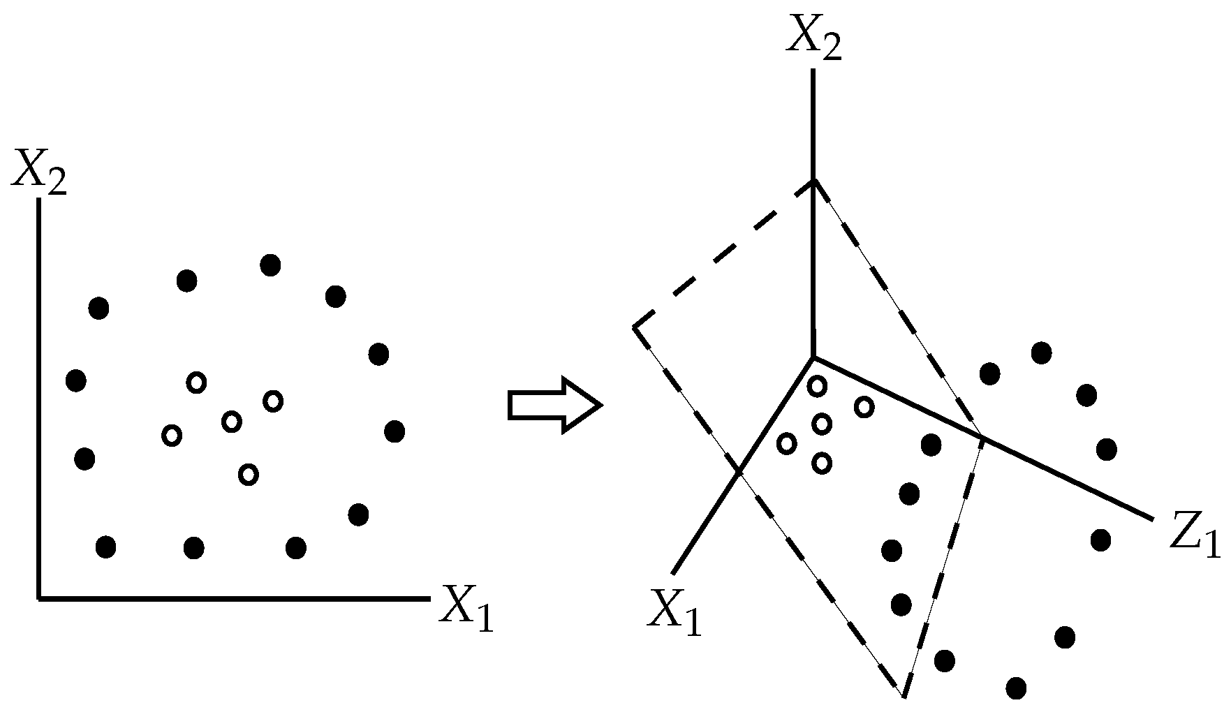
If the points that belong to different classes are not linearly separable, we may use the kernel trick, i.e., to increase dimensionality of the covariates’ universe $X_1\times X_2\times \cdots \times X_k\times T$ by one or more dimensions that could enable to find a separating hyperplane [33], as illustrated in Figure 6.

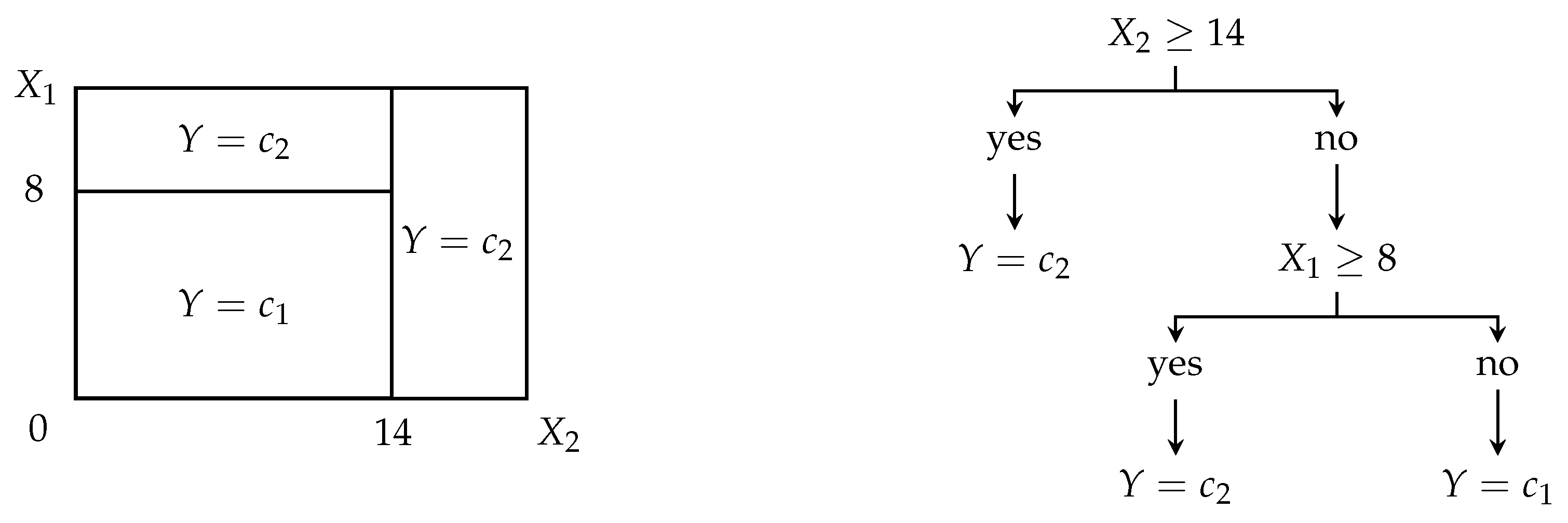
2.4.4. Decision Trees and Random Forests

Decision trees divide the universe of all covariates $X_1\times X_2\times \cdots \times X_k\times T$ into disjunctive orthogonal subspaces related to maximally probably distribution of individual classes of the target variable Y, see Figure 7 for demonstration [34].

Using node rules employing covariates and their grid-searched thresholds that minimize given criterion, e.g., deviance, entropy, or Gini index, a dataset is repeatedly split into new and new branches, while the tree containing node rules, i.e., logic formulas with the covariates and their thresholds, grows up. Once the tree is completely grown, a set of the tree’s node rules from a root node to leaves enables the classification of an individual into one of the classes $c_1$ or $c_2$.

More technically spoken, let ${\pi }_{n_{\tau },\ell }$ be a proportion of individuals that belong to class $c_{ell}$ based on node $n_{\tau }$’s rule.

If node $n_{\tau }$ is not a leaf one, then the node rule is created so that an impurity criterion $Q_{n_{\tau }}$ is minimized. The commonly used impurity criterion is

• misclassification error,

  $$Q_{n_{\tau }}=1-{\pi }_{n_{\tau },\ell },$$
• Gini index,

  $$Q_{n_{\tau }}=\sum _{\ell =1}^2{\pi }_{n_{\tau },\ell }(1-{\pi }_{n_{\tau },\ell }),$$
• and deviance (cross-entropy),

  $$Q_{n_{\tau }}=-\sum _{\ell =1}^2{\pi }_{n_{\tau },\ell }·log{\pi }_{n_{\tau },\ell }.$$

If node $n_{\tau }$ is a leaf one, then all observations that are constrained by all node rules from root one up to the leaf one $n_t$ are classified into final class $c_{\ell }^{*}\in \{c_1,c_2\}$ of target variable Y, so that

$$c_{\ell }^{*}=arg\underset{\ell \in \{1,2\}}{max}\left\{{\pi }_{n_{\tau },\ell }\right\}.$$

Decision trees natively tend to overfit the classification since, whenever there is at least one leaf node classifying into two or more classes, it is repeatedly split into two branches until each leaf node classifies just into one class. To reduce the overfitting, grown trees are pruned. A pruned subtree, derived from the grown tree, minimizes the following cost-complexity function,

$$C_{\kappa }=\sum _{n_t\in \left\{{\mathit{n}}_t\right\}}\left|\left\{{\mathit{x}}_{\mathrm{root}\to n_t}\right\}\right|·Q_{n_{\tau }}+\kappa ·\left|\left\{{\mathit{n}}_t\right\}\right|,$$

where $\left\{{\mathit{n}}_t\right\}$ is a set of all nodes in the tree, $\left\{{\mathit{x}}_{\mathrm{root}\to n_t}\right\}$ is a set of all nodes in the tree structure from the root to the leaf note $n_t$, and $\kappa$ is a tuning parameter governing the trade-off between tree complexity and size (low $\kappa$), and tree reproducibility to other similar data (high $\kappa$).

Many trees together create a random forest. To ensure that trees in a random forest are mutually independent and different enough, each tree is grown using a limited number of covariates that are selected for node rules [35]. Thus, each tree’s node might be determined using only $k^{*}<k+1$ covariates, which are randomly picked using bootstrap from $\{X_1,X_2,\dots ,X_k,T\}$, which ensures that trees of one random forest are sufficiently different one from another. A voting scheme determines the final class—an individual i is classified into class $c_{\ell }^{*}\in \{c_1,c_2\}$ which a maximum of all trees in the random forest classifies into. If there are two classes with maximum trees voting for, one is picked randomly.

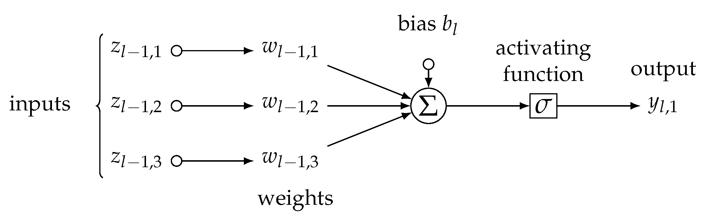
2.4.5. Artificial Neural Networks

Artificial neural networks we used in our study are weighted parallel logistic regression models [36], called neurons, as in Figure 8, following an atomic formula:

$$y_{l,j}=\sigma \left({\mathit{w}}_{l-1}^T{\mathit{z}}_{l-1}+b_l\right),$$

where $y_{l,j}$ is a signal, i.e., either 0, or 1, of j-th neuron in l-th layer of neurons aiming at the next $(l+1)$-th layer, $\sigma (•)$ is sigmoid activating function, ${\mathit{w}}_{l-1}$ is a vector of weights coming from axons of neurons in the previous $(l-1)$-th layer, $b_l$ is l-th layer’s activating threshold, and, finally, ${\mathit{z}}_{l-1}$ is a vector of incoming signals from $(l-1)$-th layer, i.e., it is either a vector of individual i’s covariates’ values ${\mathit{x}}_i={(x_{i,1},x_{i,2},\dots ,x_{i,k},t_i)}^T$ when the neurons are of the first layer ($l=1$), so it is a vector of signals ${\mathit{y}}_{l-1}={(y_{l-1,1},y_{l-1,2},\dots )}^T$ coming from $(l-1)$-th layer ($l>1$).

A number of layers and neurons in each layer are hyperparameters of the neural network’s architecture and should be chosen by an end user. Within a procedure called backpropagation, the vectors of weights ${\mathit{w}}_1,{\mathit{w}}_2,\dots$ are iteratively adjusted by a small gradient per each epoch to minimize loss functions, typically an $L_1$ or $L_2$ norm of current and previous neuron’s output $y_{l,j}$ and $y_{l,j}^{\prime }$, i.e., $|y_{l,j}^{\prime }-y_{l,j}|$ or ${|y_{l,j}^{\prime }-y_{l,j}|}^2$, respectively [37]. The learning rate determines the size of the small gradient adjusting weights in each iteration. Although many exist, the commonly applied activating function is a sigmoid one and follows a form of

$$\sigma \left(\zeta \right)=\frac{1}{1+e^{-\zeta }}.$$

In the classification framework, the number of output neurons is equal to the number of classes of target variable Y; each output neuron $y_{\{\#\mathrm{of}\mathrm{layers}\},1}$ or $y_{\{\#\mathrm{of}\mathrm{layers}\},2}$ represents one of the classes $\{c_1,c_2\}$ and final class $c_{\ell }^{*}\in \{c_1,c_2\}$ is

$$c_{\ell }^{*}=arg\underset{\ell \in \{1,2\}}{max}\left\{y_{\{\#\mathrm{of}\mathrm{layers}\},\ell }\right\}.$$

2.5. Evaluation of Classification Algorithms’ Performance

Considering individual i’s true value of variable Y, i.e., either $Y_i=c_1$, or $Y_i=c_2$, an algorithm may predict the true value correctly, ${\widehat{Y}}_i=Y_i$ or incorrectly, ${\widehat{Y}}_i\ne Y_i$. We may evaluate the performance of a classification algorithm using a proportion of a number of predicted classes equal to true classes to a number of all predicted classes. Assuming a confusion matrix [38] as in

Table 1. A confusion matrix for two true classes $Y\in \{c_1,c_2\}$ (in rows) and two predicted classes $\widehat{Y}\in \{c_1,c_2\}$ (in columns).

		Predicted Class ($\widehat{\mathit{Y}}$)
		${\mathit{c}}_{\mathbf{1}}$	${\mathit{c}}_{\mathbf{2}}$
True class ($\mathit{Y}$)	$c_1$	$n_{1,1}$	$n_{1,2}$
	$c_2$	$n_{2,1}$	$n_{2,2}$

, the number of correctly predicted classes corresponds to $n_{1,1}+n_{2,2}$, while the number of all predictions is $n_{1,1}+n_{1,2}+n_{2,1}+n_{2,2}$.

Thus, the predictive accuracy of an algorithm, i.e., what is a point estimate of the probability for which an individual’s class would be predicted correctly by the algorithm, is

$$\mathrm{accuracy}=\frac{n_{1,1}+n_{2,2}}{n_{1,1}+n_{1,2}+n_{2,1}+n_{2,2}}=\frac{{\sum }_{i=1}^2{n}_{i,i}}{{\sum }_{i=1}^2{\sum }_{j=1}^2{n}_{i,j}}.$$

(18)

Even more, assuming that classes $Y_i=c_2$ and ${\widehat{Y}}_i=c_2$ are of “positive” meaning or are of our special interest, then [39], the precision is a point estimate of the probability that an individual classified to ${\widehat{Y}}_i=c_2$ class is truly of class $Y_i=c_2$, so

$$\mathrm{precision}=P\left(Y_i=c_2|{\widehat{Y}}_i=c_2\right)=\frac{P\left(Y_i=c_2\wedge {\widehat{Y}}_i=c_2\right)}{P\left({\widehat{Y}}_i=c_2\right)}=\frac{n_{2,2}}{n_{1,2}+n_{2,2}},$$

(19)

and the recall is a point estimate of the probability that an individual belonging to class $Y_i=c_2$ is classified to class ${\widehat{Y}}_i=c_2$,

$$\mathrm{recall}=P\left({\widehat{Y}}_i=c_2|Y_i=c_2\right)=\frac{P\left({\widehat{Y}}_i=c_2\wedge Y_i=c_2\right)}{P\left(Y_i=c_2\right)}=\frac{n_{2,2}}{n_{2,1}+n_{2,2}}.$$

(20)

Putting the precision and recall together, so-called F1 score is of form,

$$\mathrm{F}1 \mathrm{score}=2·\frac{\mathrm{precision}·\mathrm{recall}}{\mathrm{precision}+\mathrm{recall}},$$

(21)

and, inspecting Formula (21) above, since F1 score keeps balance between the precision and recall, it is sometimes considered as a metric of an overall model predictive performance [39].

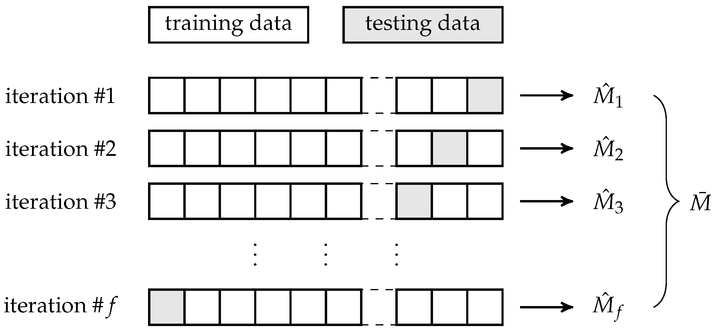
To avoid any bias in the performance measures’ estimation, we estimate them multiple times using f-fold cross-validation [40], see Figure 9. Before each iteration of the f-fold cross-validation, the entire dataset is split into two parts following a ratio $(f-1):1$ for training and testing subset, respectively, where $f\in \mathbb{N}$ and $f>1$. Within each iteration, a portion of $\frac{f-1}{f}$ of all data are used for training of an algorithm, while the remaining $\frac{1}{f}$ portion of all data are used for testing a model based on the trained algorithm.

The j-th iteration of the f-fold cross-validation outputs a defined estimate ${\widehat{M}}_j$ of a performance metric, so, in our case, $M\in \{\mathrm{accuracy}, \mathrm{precision}, \mathrm{recall}, \mathrm{F}1\mathrm{score}\}$ following Formulas (18)–(21). The estimates are eventually averaged to obtain a more robust estimate

$$\overline{M}=\frac{1}{f}\sum _{j=1}^f{\widehat{M}}_j,$$

thus, in our case,

$$\begin{array}{cc}\hfill \overline{\mathrm{accuracy}}& =\frac{1}{f}\sum _{j=1}^f{\widehat{\mathrm{accuracy}}}_j,\hfill \\ \hfill \overline{\mathrm{precision}}& =\frac{1}{f}\sum _{j=1}^f{\widehat{\mathrm{precision}}}_j,\hfill \\ \hfill \overline{\mathrm{recall}}& =\frac{1}{f}\sum _{j=1}^f{\widehat{\mathrm{recall}}}_j,\hfill \\ \hfill \overline{\left\{\mathrm{F}1\mathrm{score}\right\}}& =\frac{1}{f}\sum _{j=1}^f{\widehat{\left\{\mathrm{F}1\mathrm{score}\right\}}}_j.\hfill \end{array}$$

Finally, considering all f iterations of the f-fold cross-validation, we also report a confusion matrix containing medians of numbers of matches and mismatches between true classes Y and predicted ones $\widehat{Y}$. Using the matrix in Table 1, the median confusion matrix is the matrix in

Table 2. A median confusion matrix for two true classes $Y\in \{c_1,c_2\}$ (in rows) and two predicted classes $\widehat{Y}\in \{c_1,c_2\}$ (in columns). Assuming that value ${}_1{n}_{i,j}$ comes from the 1-st iteration, value ${}_2{n}_{i,j}$ comes from the 2-nd iteration, …, value ${}_f{n}_{i,j}$ comes from the f-th iteration, then ${\tilde{n}}_{i,j}$ is median over values $\{{}_1{n}_{i,j},{}_2{n}_{i,j},\dots ,{}_f{n}_{i,j}\}$.

		Predicted Class ($\widehat{\mathit{Y}}$)
		${\mathit{c}}_{\mathbf{1}}$	${\mathit{c}}_{\mathbf{2}}$
True class ($\mathit{Y}$)	$c_1$	${\tilde{n}}_{1,1}$	${\tilde{n}}_{1,2}$
	$c_2$	${\tilde{n}}_{2,1}$	${\tilde{n}}_{2,2}$

, where ${\tilde{n}}_{i,j}$ for $\forall i\in \{1,2\}$ and $\forall j\in \{1,2\}$ is median value over all values $n_{i,j}$ from the 1-st, 2-nd, …, f-th iteration of the f-fold cross-validation.

Summation of each median confusion matrix should be approximately equal to a portion $\frac{1}{f}$ of all data since each median confusion matrix is produced by the testing, i.e., predicting procedure within an iteration of f-fold cross-validation.

2.6. Asymptotic Time Complexity of Proposed Prediction Based on Time-to-Event Variable Decomposition

Let us briefly analyze the asymptotic time complexity of the proposed method, i.e., the time-to-event variable decomposition and prediction of an event of interest’s occurrence in time using time and event components, covariates, and machine-learning classification algorithms.

Assuming we have $n\in \mathbb{N}$ individuals in a dataset in total, time-to-event variable decomposition is a unit time operation made for each of them, so its asymptotic time complexity, using Bachmann–Landau notation [41], is $\mathrm{\Theta }\left(n\right)$. Picking a machine-learning classifier, let us suppose that it takes $\mathrm{\Theta }\left(\lambda \right(n\left)\right)$ time when training on n observations (and all their covariates’ values), whereas it takes $\mathrm{\Theta }\left(\pi \right(n\left)\right)$ time if testing or predicting an output for n observations (both testing and predicting procedures could be considered the same regarding their asymptotic time complexity since they use a trained model and only output target variable values for input). Firstly, the training, testing, and prediction are linear procedures with respect to a number of observations, i.e., training, testing, or prediction considering $2n$ observations would take approximately double the time than considering only n observations.

$$\begin{array}{l}\mathrm{\Theta }\left(\lambda \right(\ell n\left)\right)\approx \mathrm{\Theta }(\ell ·\lambda (n\left)\right)\approx \ell ·\mathrm{\Theta }\left(\lambda \right(n\left)\right)\\ \mathrm{\Theta }\left(\pi \right(\ell n\left)\right)\approx \mathrm{\Theta }(\ell ·\pi (n\left)\right)\approx \ell ·\mathrm{\Theta }\left(\pi \right(n\left)\right),\end{array}$$

(22)

however, using Bachmann–Landau logic, linear multipliers do not change asymptotic time complexity, so it is as well

$$\begin{array}{l}\ell ·\mathrm{\Theta }\left(\lambda \right(n\left)\right)\approx \mathrm{\Theta }\left(\lambda \right(n\left)\right)\\ \ell ·\mathrm{\Theta }\left(\pi \right(n\left)\right)\approx \mathrm{\Theta }\left(\pi \right(n\left)\right).\end{array}$$

(23)

In addition, we may assume that training a model is generally not faster than testing a model or using it for prediction, considering n observations, so

$$\mathrm{\Theta }\left(\lambda \right(n\left)\right)\gtrsim \mathrm{\Theta }\left(\pi \right(n\left)\right)$$

and neither training nor testing nor even predicting considering n observations is faster than n-times performed unit time operation, so

$$\mathrm{\Theta }\left(\lambda \right(n\left)\right)\gtrsim \mathrm{\Theta }\left(\pi \right(n\left)\right)\gtrsim \mathrm{\Theta }\left(n\right).$$

(24)

Applying derivations from the previous section, within each iteration of f-fold cross-validation, we build a model on $\frac{f-1}{f}n$ portion of the dataset, test it on $\frac{1}{f}n$ portion of the dataset. This is repeated $f\in \mathbb{N}$ times since there are f iterations in the f-fold cross-validation. Thus, applied to n observations, the time-to-event variable decomposition, f-fold cross-validation containing training and testing all f models and prediction on output, respectively, would asymptotically take $\mathrm{\Theta }(•)$, such that

$$\begin{array}{cc}\hfill \mathrm{\Theta }(•)& \approx \mathrm{\Theta }\left(n\right)+f·\left(\mathrm{\Theta }\left(\lambda \left(\frac{f-1}{f}n\right)\right)+\mathrm{\Theta }\left(\pi \left(\frac{1}{f}n\right)\right)\right)+\mathrm{\Theta }\left(\pi \left(n\right)\right)\stackrel{\left(22\right)}{\approx }\hfill \\ \hfill & \stackrel{\left(22\right)}{\approx }\mathrm{\Theta }\left(n\right)+f·\left(\frac{f-1}{f}·\mathrm{\Theta }\left(\lambda \left(n\right)\right)+\frac{1}{f}·\mathrm{\Theta }\left(\pi \left(n\right)\right)\right)+\mathrm{\Theta }\left(\pi \left(n\right)\right)\approx \hfill \\ \hfill & \approx \mathrm{\Theta }\left(n\right)+(f-1)·\mathrm{\Theta }\left(\lambda \left(n\right)\right)+\mathrm{\Theta }\left(\pi \left(n\right)\right)+\mathrm{\Theta }\left(\pi \left(n\right)\right)\stackrel{\left(23\right)}{\approx }\hfill \\ \hfill & \stackrel{\left(23\right)}{\approx }\mathrm{\Theta }\left(\lambda \left(n\right)\right)+\mathrm{\Theta }\left(\pi \left(n\right)\right)+\mathrm{\Theta }\left(n\right),\hfill \end{array}$$

(25)

so, improving Formula (25), it is obviously

$$\begin{array}{cc}\hfill \mathrm{\Theta }(•)& \approx \mathrm{\Theta }\left(\lambda \left(n\right)\right)+\mathrm{\Theta }\left(\pi \left(n\right)\right)+\mathrm{\Theta }\left(n\right)\gtrsim \hfill \\ \hfill & \gtrsim \mathrm{\Theta }\left(\lambda \left(n\right)\right)\hfill \end{array}$$

(26)

and also

$$\begin{array}{cc}\hfill \mathrm{\Theta }(•)& \approx \mathrm{\Theta }\left(\lambda \left(n\right)\right)+\mathrm{\Theta }\left(\pi \left(n\right)\right)+\mathrm{\Theta }\left(n\right)\stackrel{\left(24\right)}{\lesssim }\hfill \\ \hfill & \stackrel{\left(24\right)}{\lesssim }\mathrm{\Theta }\left(\lambda \left(n\right)\right)+\mathrm{\Theta }\left(\lambda \left(n\right)\right)+\mathrm{\Theta }\left(\lambda \left(n\right)\right)\approx \hfill \\ \hfill & \approx 3·\mathrm{\Theta }\left(\lambda \left(n\right)\right)\stackrel{\left(23\right)}{\approx }\hfill \\ \hfill & \stackrel{\left(23\right)}{\approx }\mathrm{\Theta }\left(\lambda \left(n\right)\right).\hfill \end{array}$$

(27)

Putting Formulas (26) and (27) together, we obtain

$$\mathrm{\Theta }\left(\lambda \left(n\right)\right)\gtrsim \mathrm{\Theta }(•)\gtrsim \mathrm{\Theta }\left(\lambda \left(n\right)\right);$$

thus,

$$\mathrm{\Theta }(•)\approx \mathrm{\Theta }\left(\lambda \left(n\right)\right),$$

and, finally, asymptotic time complexity $\mathrm{\Theta }(•)$ of the time-to-event decomposition, followed by prediction of an event of interest’s occurrence in time using machine-learning classification algorithms is approximately equal to asymptotic time complexity of training of the classification algorithm, regardless of its kind. In other words, the proposed method does not take significantly longer computational time when performed from beginning to end than the classifier used within the technique.

2.7. Description of Used Dataset

The dataset used to confirm the proposed methodology’s feasibility comes from the Department of Occupational Medicine, University Hospital Olomouc. The data contain covariates’ values in about COVID-19 non-vaccinated 663 patients; there are 34 covariates describing COVID-19 antibody blood level values and their decrease below laboratory cut-off for IgG and IgM antibodies in various time points and multiple biometric and other variables, continuous and categorical. All patients have been informed in advance about using their data for the study, following ideas of Helsinki’s declaration [42].

Regarding the covariates, there are

• continuous variables such as age (in years), weight (in kilograms), height (in centimeters), body mass index (in kilogram per squared meters), COVID-19 IgG antibody blood level, COVID-19 IgM antibody blood level, a total count of COVID-19 defined symptoms, the time between beginning and end of COVID-19 symptoms (in days), the time between laboratory-based proof of COVID-19 and antibody blood sampling (in days), the time between COVID-19 symptoms’ offset and antibody blood sampling (in days);
• categorical variables such as sex (male/female), COVID-19 IgG antibody blood level decrease below laboratory cut-off (yes/no), COVID-19 IgM antibody blood level decrease below laboratory cut-off (yes/no), COVID-19 defined symptoms such as headache (yes/no), throat pain (yes/no), chest pain (yes/no), muscle pain (yes/no), dyspnea (yes/no), fever (yes/no), subfebrile (yes/no), cough (yes/no), lack of appetite (yes/no), diarrhea (yes/no), common cold (yes/no), fatigue (yes/no), rash (yes/no), loss of taste (yes/no), loss of smell (yes/no), nausea (yes/no), mental troubles (yes/no), and insomnia (yes/no).

As a time-to-event variable, a COVID-19 IgG antibody blood level decrease below the laboratory cut-off or COVID-19 IgM antibody blood level decrease below the laboratory cut-off, respectively, is considered the event component. In contrast, the time between laboratory-based proof of COVID-19 and antibody blood sampling is taken into account for the time component.

3. Results

We applied the Cox proportional hazard model and proposed methodology handling time-to-event decomposition and classification on the dataset as described in the previous sections. All computations were performed using R statistical and programming language [43].

Firstly, we performed and built the Cox proportional hazard model, considering COVID-19 antibody blood level decrease or non-decrease below laboratory cut-off (for IgG and IgM antibodies, respectively) as an event of interest that does or does not occur when antibody blood sampling is carried out a varying time period after COVID-19 symptoms’ onset is laboratory proven.

Assuming Cox proportional hazard model for the prediction of COVID-19 IgG antibody blood level decrease or non-decrease below laboratory cut-off, the prediction of IgG antibody decrease below the cut-off was repeated ten times within 10-fold cross-validation and output the predictive accuracy about $0.796$, precision about $0.889$, recall of $0.951$, and F1 score about $0.884$; see

Table 3. Predictive accuracy, precision, recall and F1 score of COVID-19 IgG antibody blood level decrease below laboratory cut-off’s estimation for the listed algorithms, both traditional Cox’s model and classifiers using a decomposed time-to-event variable, calculated using 10-fold cross-validation.

Algorithm	Predictive Accuracy	Precision	Recall	F1 Score
Cox proportional hazard model	0.796	0.889	0.951	0.884
multivariate logistic regression	0.811	0.820	0.984	0.894
naïve Bayes classifier	0.771	0.841	0.896	0.865
support vector machines	0.845	0.845	1.000	0.913
decision trees	0.783	0.833	0.920	0.874
random forests	0.836	0.850	0.980	0.908
artificial neural networks	0.806	0.827	0.953	0.881

. The median confusion matrix for Cox proportional hazard model predicting IgG antibody decrease below cut-off is in Figure 10. An average value of threshold $p_{\mathrm{threshold}}$ over all iterations of 10-fold cross-validation for IgG decrease prediction was about ${\overline{p}}_{\mathrm{threshold}}=0.070$. Cox proportional hazard model predicted COVID-19 IgM antibody blood level decrease or non-decrease below laboratory cut-off with predictive accuracy $0.627$, precision of $0.598$, recall of $0.519$ and F1 score about $0.507$; see

Table 4. Predictive accuracy, precision, recall and F1 score of COVID-19 IgM antibody blood level decrease below laboratory cut-off’s estimation for the listed algorithms, both traditional Cox’s model and classifiers using a decomposed time-to-event variable, calculated using 10-fold cross-validation.

Algorithm	Predictive Accuracy	Precision	Recall	F1 Score
Cox proportional hazard model	0.627	0.598	0.519	0.507
multivariate logistic regression	0.578	0.530	0.429	0.468
naïve Bayes classifier	0.574	0.532	0.373	0.428
support vector machines	0.527	0.506	0.347	0.393
decision trees	0.583	0.551	0.412	0.461
random forests	0.555	0.556	0.419	0.467
artificial neural networks	0.516	0.443	0.402	0.518

. The median confusion matrix for Cox proportional hazard model predicting IgM antibody decrease below cut-off is in Figure 11. An average threshold $p_{\mathrm{threshold}}$ over 10-fold cross-validation’s iterations when IgM decrease predicted was about ${\overline{p}}_{\mathrm{threshold}}=0.765$.

Let us proceed to the proposed technique. Supposing multivariate logistic regression as a tool for the prediction of COVID-19 IgG antibody blood level decrease or non-decrease below laboratory cut-off, the prediction of IgG antibody decrease was repeated ten times within 10-fold cross-validation and ended with the predictive accuracy about $0.811$, precision about $0.820$, recall of $0.984$, and F1 score about $0.894$, see Table 3. The median confusion matrix for multivariate logistic regression predicting IgG antibody decrease below cut-off is in Figure 10. Multivariate logistic regression predicted COVID-19 IgM antibody blood level decrease or non-decrease below laboratory cut-off with predictive accuracy $0.578$, precision about $0.530$, recall of $0.429$, and F1 score about $0.468$, see Table 4. The median confusion matrix for multivariate logistic regression predicting IgM antibody decrease below cut-off is in Figure 11.

Naïve Bayes classifier, when predicting COVID-19 IgG antibody blood level decrease or non-decrease below laboratory cut-off, was repeated ten times within 10-fold cross-validation and returned the predictive accuracy about $0.771$, precision about $0.841$, recall of $0.896$, and F1 score about $0.865$; see Table 3. The median confusion matrix for the naïve Bayes classifier predicting IgG antibody decrease below cut-off is in Figure 10. Naïve Bayes classifier predicted COVID-19 IgM antibody blood level decrease or non-decrease below laboratory cut-off with predictive accuracy $0.574$, precision about $0.532$, recall of $0.373$, and F1 score about $0.428$, see Table 4. The median confusion matrix for naïve Bayes classifier predicting IgM antibody decrease below cut-off is in Figure 11.

When support vector machines using nonlinear kernel trick were considered for prediction of COVID-19, IgG antibody blood level decrease or non-decrease below laboratory cut-off, the algorithm ended with the predictive accuracy about $0.845$, precision about $0.845$, recall of $1.000$, and F1 score about $0.913$; see Table 3. The median confusion matrix for support vector machines predicting IgG antibody decrease below cut-off is in Figure 10. Support vector machines predicted COVID-19 IgM antibody blood level decrease or non-decrease below laboratory cut-off with predictive accuracy $0.527$, precision about $0.506$, recall of $0.347$, and F1 score about $0.393$; see Table 4. The median confusion matrix for support vector machines predicting IgM antibody decrease below cut-off is in Figure 11.

Decision trees predicted COVID-19 IgG antibody blood level decrease or non-decrease below laboratory cut-off using 10-fold cross-validation with the predictive accuracy about $0.783$, precision of $0.833$, recall of $0.920$, and F1 score about $0.874$, see Table 3. The pruning parameter we used for model training has been adopted from default and recommended setting, i.e., $\kappa =0.01$. The median confusion matrix for decision trees predicting IgG antibody decrease below cut-off is in Figure 10. Decision trees predicted COVID-19 IgM antibody blood level decrease or non-decrease below laboratory cut-off with predictive accuracy $0.583$, precision about $0.551$, recall of $0.412$, and F1 score about $0.461$, see Table 4. The median confusion matrix for decision trees predicting IgM antibody decrease below cut-off is in Figure 11.

Random forests were also repeated ten times within 10-fold cross-validation to predict COVID-19 IgG antibody blood level decrease or non-decrease below laboratory cut-off. Each model of the random forests consisted of 1000 decision trees. The random forests’ predictive accuracy of IgG antibody decrease below cut-off is about $0.836$, precision about $0.850$, recall of $0.980$, and F1 score about $0.908$; see Table 3. The median confusion matrix for random forests predicting IgG antibody decrease below cut-off is in Figure 10. Random forests predicted COVID-19 IgM antibody blood level decrease or non-decrease below laboratory cut-off with predictive accuracy $0.555$, precision about $0.556$, recall of $0.419$, and F1 score about $0.467$; see Table 4. The median confusion matrix for random forests predicting IgM antibody decrease below cut-off is in Figure 11.

Finally, artificial neural networks with backpropagation, we performed ten times within 10-fold cross-validation to predict COVID-19 IgG antibody blood level decrease or non-decrease below laboratory cut-off, output the predictive accuracy of IgG antibody decrease below cut-off about $0.806$, precision about $0.827$, recall of $0.953$, and F1 score about $0.881$; see Table 3. For each iteration of the 10-fold cross-validation, we used two hidden layers with 10 and 5 neurons, respectively, and set the learning rate to an interval of approximately $-0.10$ to $+0.30$. The median confusion matrix for artificial neural networks predicting IgG antibody decrease below cut-off is in Figure 10. Artificial neural networks predicted COVID-19 IgM antibody blood level decrease or non-decrease below laboratory cut-off with predictive accuracy $0.516$ precision about $0.443$, recall of $0.402$, and F1 score about $0.518$; see Table 4. The median confusion matrix for artificial neural networks predicting IgM antibody decrease below cut-off is in Figure 11.

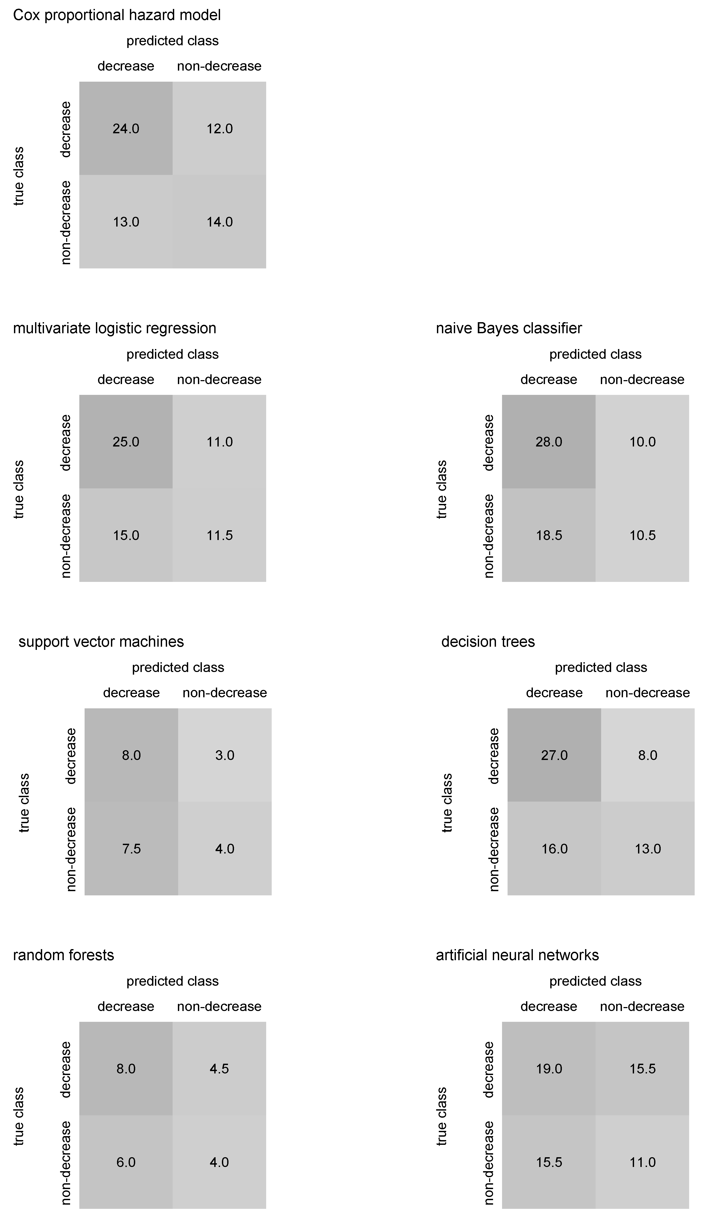
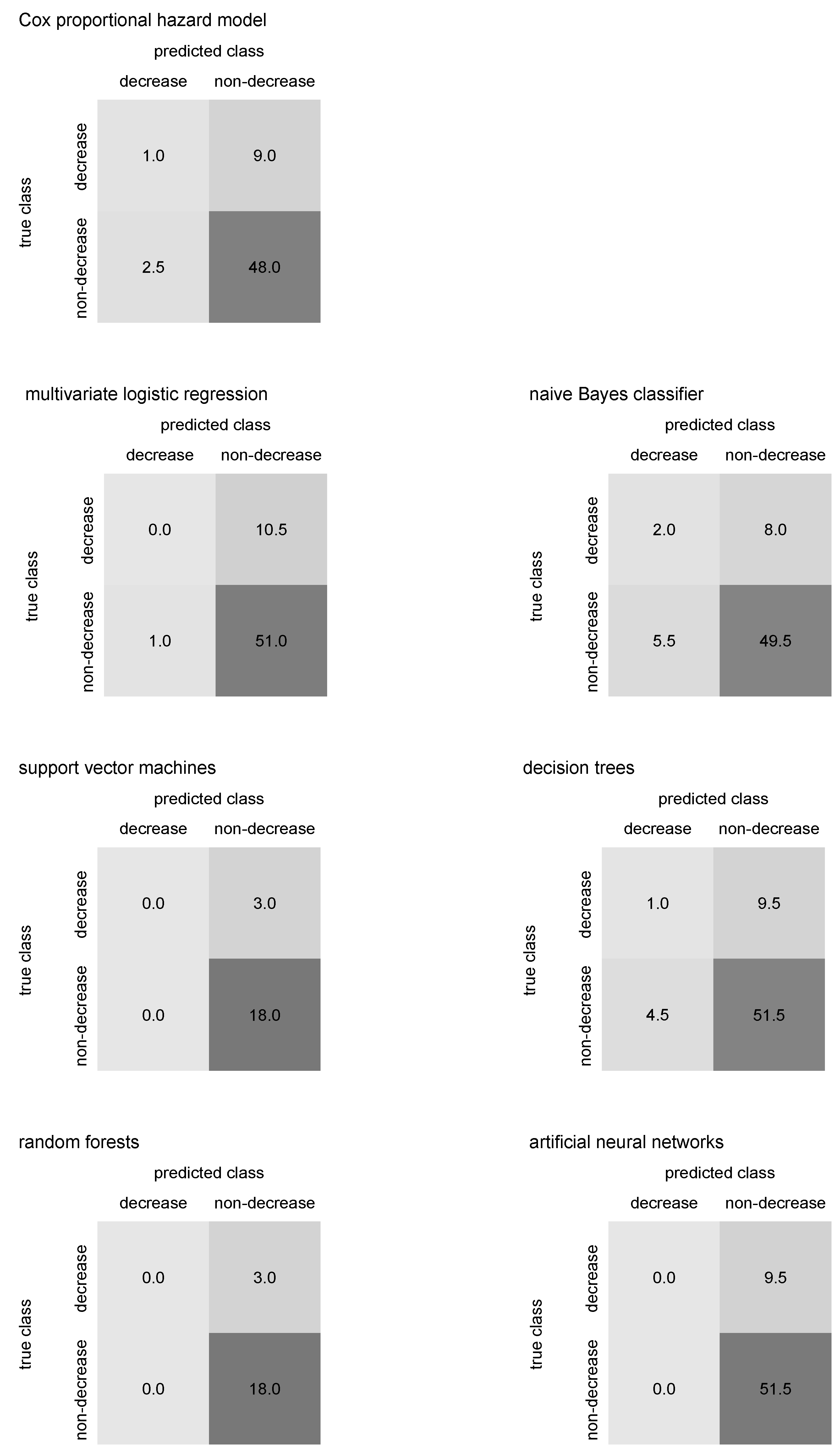
Median confusion matrices in Figure 10 and Figure 11 may help to identify whether an algorithm predicting COVID-19 antibody blood level decrease below laboratory cut-off tends to over- or underestimate the antibody decrease. Thus, comparing predicted numbers for antibody blood decrease and non-decrease in the median confusion matrices columns could be useful.

4. Discussion

Prediction of the time period till an event of interest is the most challenging and essential task in statistics, particularly when the event has a significant impact on an individual’s life. Without a doubt, the blood level of antibodies against COVID-19 and their development in time, especially their decrease below laboratory cut-off, also called seronegativity, could determine how an individual would face COVID-19 infection when exposed to it. This is one of the reasons we wanted to compare traditional statistical techniques and machine-learning-based approaches on antibody blood level decrease just for the diagnosis of COVID-19.

Survival analysis provides a toolbox of classical methods that model and predict the time to event. Many methods are commonly used regardless of whether they meet their formal assumptions when applied to real data. Since these methods, including the Cox proportional hazard model for prediction of the time to event, handle the relatively advanced concept of time-to-event modeling, they are limited by relatively strict statistical assumptions. Fortunately, there are various alternatives for how to address the issue of assumptions violation; in the case of the Cox proportional hazard model, we may use rather stratified models that partition an input dataset into multiple parts and build models for them independently, or we might prefer to perform other time-varying and time-partitioning that split the hazard function into several consecutive parts and model the parts individually.

In addition, machine-learning approaches could predict in a time-to-event fashion. A promising fact about the application of machine-learning algorithms not only in survival analysis is that these algorithms usually have very relaxed or not at all prior statistical assumptions. However, the majority of works and papers that employ machine-learning-based techniques for purposes of survival analyses often use mixed methods that combine features from survival analysis and machine-learning, namely scoring and counting models [44], linear-separating survival models such as survival random forests [45], or discrete-time survival models [46]. Nevertheless, if the papers predicted the time to an event of interest and use comparable metrics of performance [47], regardless of data focus, they usually reach predictive accuracy of about 0.7–0.9. These are similar predictive accuracy values we have obtained using the proposed time-to-event decomposition and ongoing classification too. Besides the Cox proportional hazard model, there are parametric survival models such as Weibull or log-normal ones. Those are flexible and might work well on real-world data; however, they require an initial assumption on the parametric choice of the baseline hazard function. If the assumption is wrong, predictions could fail. For example, Valvo in [48] predicts COVID-19-related deaths (instead of antibody decrease) using a log-normal survival model with an average error of about 20%, which is, although a different topic, a similar value to our results.

Going deeper into machine learning applied for prediction in COVID-19 diagnosis, many papers deal with predictions of COVID-19 symptoms’ offset, COVID-19 recurrence, long-term COVID-19 disease, post-COVID-19 syndrome [49,50,51]. However, all the mentioned topics of prediction related to COVID-19 manifestation are usually based on datasets that consist of individual observations of symptoms, biometric data, and laboratory or medical imaging data. Thus, very often, the data size is very large, so machine learning is a legit way for how to analyze these kinds of data; a time-to-event variable is generally missing, so such data are not suitable for survival analysis, though. This may be why papers applying machine-learning prediction on survival data related to COVID-19 are not as frequent as we could initially expect, considering the importance of the topic, or publicly available data are usually aggregated up to a higher level, which is generally not an optimal starting point for survival analysis. Furthermore, some publications are still estimating COVID-19 blood antibody level’s development in time [52,53,54], but using traditional methods, so not applying time-to-event decomposition.

Of papers dealing with COVID-19-related predictions using machine-learning techniques, Willette et al. [55] predicted the risk of COVID-19 severity and risk of hospitalization due to COVID-19, respectively, using discriminant and classification algorithms applied on 7539 observations (!) with variable similar to ours, and received an accuracy of about $0.969$ and $0.803$, respectively. While our dataset is more than ten times smaller, we obtained similar results. Kurano et al. [56] employed XGBoost (extreme gradient boosting) to classify COVID-19 severity using immunology-related variables. Applied on 134 patients, they received a predictive accuracy between $0.380$–$0.900$ for various lengths of symptoms’ onset. Using standard explanatory variables, Singh et al. [57] performed support vector machines to determine infectious COVID-19 status on 1063 recipients with final accuracy greater than $0.700$. In addition, Rostami and Oussalah [58] combined feature selectors with explainable trees and others to predict COVID-19 diagnosis. Applied to available 5644 patients’ blood test data containing 111 features, they received an accuracy of about $0.877$ for XGBoost, about $0.848$ for support vector machines, about $0.853$ for neural networks, and $0.884$ for explainable decision trees, respectively. Cobre at al. [59] introduced a new method for COVID-19 severity, combining various algorithms such as artificial neural networks, decision trees, discriminant analysis, and k-nearest neighbor. Applied on biochemical tests of 5643 patients, they obtained a predictive accuracy of about $0.840$. Albeit no COVID-19-related predictions, but classification into acute organ injury or non-acute organ injury, Duan et al. [60] received precision and recall slightly above $0.800$, using about 20 features of 339 patients. Thus, the predictive performance we obtained using our proposed method seems comparable with the literature.

However, according to our expectations, when sample sizes, as well as the numbers of features, are enormous and machine-learning algorithms could return outstanding results, as Bhargava et al. [61] showed when they predicted COVID-19 disease using nine large datasets combining laboratory and imaging data and designed the algorithms in deep-learning fashion. As a result, they received an accuracy above $0.900$, or, using ensembled algorithms, even close to $0.990$.

Our proposed method, based on time-to-event decomposition and machine-learning classification of individuals to an event of interest’s occurrence or non-occurrence, using the time to event as an explanatory covariate, might contribute to the application of machine-learning for survival-like prediction in COVID-19 patients. Surely we do not want to claim that the method we are introducing in the paper would work on each dataset of similar size; however, thanks to a robust estimate of the predictive accuracy using 10-fold cross-validation, we may believe that the results we have obtained are not only random but supported by sufficient evidence of perfomance metrics and method’s properties.

Considering the IgG antibodies and their blood level decrease below laboratory cut-off in our patients, all performed algorithms show satisfactory performance and output relatively promising results regarding the predictive accuracy, as figured in Table 3. The Cox proportional hazard model, taking into account as a golden standard, reported similar predictive accuracies such as multivariate logistic regression, naïve Bayes classifier, and decision trees. An assumption of the Cox model that survival curves for various combinations of covariates’ values should be met—particularly, survival curves would not cross each other or drop to zero, as plotted in Figure 1 and Figure 2. The multivariate logistic regression is a “baseline” model that performs well in prediction but might suffer from multicollinearity between covariates [62]. Naïve Bayes classifier is a relatively simple algorithm and often outputs surprisingly good results; however, it depends on only one assumption, but its performance could be ruined if it is violated—explanatory covariates should be independent, as applied in Formula (17). Decision trees are practically assumption-free [63] but become more powerful when creating an entire random forest model. Support vector machines and random forests seem to noticeably outperform the Cox model in predictive accuracy, precision, recall, and F1 score—both algorithms reached all metrics higher than Cox’s regression using our dataset. The support vector machines are sophisticated algorithms. Using the kernel trick, these can find a separating hyperplane even for linear non-separable points of different classes. The random forest is the only algorithm among others that is natively ensembled, i.e., consists of a large number of other classification algorithms—decision trees. This is why the random forest typically shows good predictive performance. Among all algorithms applied to the data and predicting IgG antibody decrease, artificial neural networks reported the predictive performance slightly better than the Cox’s model—neural networks are universal classifiers, and their performance could be even improved when larger subsets are used for training, different activating function applied or various architecture of hidden layers investigated. Performance metrics other than predictive accuracy, as listed in Table 3, are more than satisfying too—and each of them is greater than $0.800$.

Prediction of IgM antibody decrease might be tricky since IgM antibodies are less related to a cause it induced their growth, i.e., COVID-19 exposure [64]. This might be why all algorithms performed mutually similar (and relatively poor) outputs of predictive accuracy and other metrics, as reported in Table 4.

In the case of IgG decrease prediction, support vector machines, random forest, and neural networks do not predict the decrease class; however, the number of individuals with antibody decrease is significantly lower than those with no antibody decrease, see Figure 10, so the predictive accuracy is not affected. Still, the possible lack of data in the “IgG decrease” class in training sets could cause the mentioned algorithms to fail to classify a few individuals from the class correctly. Mainly, neural networks are sensitive to this. If the median confusion matrix summation in Figure 10 and Figure 11 is lower than approximately one-tenth of the entire dataset size, then the antibody decrease is likely not predicted for some individuals. This could happen due to their missing covariates’ values, which occurred for the three previously mentioned algorithms. Inspecting median confusion matrices in Figure 11, there seems to be no algorithm that would fail in the prediction of one of the classes in IgM antibody decrease. However, in general, the accuracy of IgM decrease is relatively low, likely caused by the advanced complexity of IgM (!) decrease prediction (compared to IgG decrease prediction).

As for the limitation of the work, the fact that the proposed methodology works with good performance, particularly for IgG antibody decrease prediction, does not guarantee that it would work on another dataset with similar or even better performance. In addition, classification into classes that stand for an event of interest’s occurrence and non-occurrence consider both classes equal, which sidelines the censoring; however, it seems not to affect prediction performance. In addition, when the classifiers are mutually compared within the proposed method, one should take into account the fact that some of the algorithms did not classify all observations, as we see in Figure 10 and Figure 11 (i.e., when the summation of a median confusion matrix is less than one-tenth of the dataset), and consider such a comparison rather only as approximative. Machine-learning classification algorithms within the proposed method may bias any inference potentially carried out using the event of interest’s occurrence estimates [65]—in this article, we are primarily interested in prediction paradigm and predictive performance. Finally, albeit not a limitation, but rather a note, varying tuning parameters set for classifiers in the introduced method and different sample sizes used for classifiers’ training, testing, and predicting may lead to other predictive performances.

5. Conclusions

Whether an individual would likely experience an event of interest or not, and if so, when exactly, is an essential predictive task in survival analysis. Unfortunately, statistical assumptions often limit methods commonly used to perform this forecasting.

In this work, we address the issue of assumption violation and employ machine learning, usually assumption-free or assumption-relaxed, in the predictive task. We decompose the time-to-event variable into two components—a time and an event one. While the event component is classified using various machine-learning classification algorithms, the time component becomes one of the covariates on the input of the classification models. Classifying into an event of interest’s occurrence and non-occurrence enables us to compare our proposed method with the traditional Cox proportional hazard model.

We apply the introduced methodology to COVID-19 antibody data where we predict IgG and IgM antibody blood level decrease below laboratory cut-off, also considering other explanatory covariates besides the time component.

The asymptotic time complexity of the proposed method equals the computational time of a classifier employed in the method. Compared to the Cox model, the classification does not take into account any censoring and considers both classes, i.e., an event of interest occurrence and non-occurrence, as equal. However, predictive performance measured using predictive accuracy and other metrics is for some models, particularly when IgG antibody decrease is estimated, higher than for the Cox model. Namely, multivariate logistic regression (with an accuracy of $0.811$), support vector machines (with an accuracy of $0.845$), random forests (with an accuracy of $0.836$), and artificial neural networks (with an accuracy of $0.806$) seem to outperform the Cox’s regression (with an accuracy of $0.796$), applied as classifiers in the proposed method on the COVID-19 data and predicting IgG antibody decrease below the cut-off. The precision, recall, and F1 score of the four named classifiers are constantly high, generally above $0.800$. Regarding IgM antibody decrease below cut-off, Cox’s regression and the proposed method employing various classifiers perform relatively poorly, likely due to a weak association between COVID-19 exposure and IgM antibody production. In comparison, Cox’s model reached an accuracy of about $0.627$, and all classifiers within the introduced method predicted with an accuracy of about $0.520$–$0.583$.

The proposed method seems to be a promising tool, currently applied to COVID-19 IgG antibody decrease prediction. Since IgG antibodies are closely related to protection against COVID-19 disease, an effective and accurate forecast of their (non-)decrease below laboratory cut-off could help—with no explicit need for time-consuming and expensive blood testing—to early identify COVID-19 non-vaccinated individuals with sufficient antibody level that could not undergo boosting vaccination when new COVID-19 outbreak incomes, or the non-vaccinated with IgG antibody decrease could be detected early as in risk of severe COVID-19, using only the algorithm and variables from their case history.

As for the future outlook, the proposed method could benefit from ensembled classifiers, increasing their predictive accuracy. In addition, various tuning parameters’ settings might improve predictive performance. Probably, the proposed method broadly applies to similar problems based on two-states survival prediction tasks.