Abstract
Particle-reinforced metals are being developed for advanced heat dissipation applications. However, an irregularly shaped void develops during eutectic solidification and enhances interfacial stress induced by visco-plastic deformation in temperature gradient conditions. An analytical solution to an irregularly shaped coated hole embedded in an infinite substrate under an arbitrarily located heat source or sink is presented. For a coated polygonal hole with any number of edges, a rapidly convergent series solution of the temperature and stress functions is expressed in an elegant form using conformal mapping, the analytic continuation theorem, and the alternation method. The iterations of the trial-and-error method are utilized to obtain the solution for the correction terms. First, temperature contours are obtained to provide an optimal suggestion that a larger thermal conductivity of the coating layer exhibits better heat absorption capacity. Furthermore, interfacial stresses between a coating layer and substrate increase if the strength of a point thermal singularity and thermal mismatch increases. This study provides a detailed explanation for the growth of an irregular void at an ambient temperature gradient.
MSC:
74S70
1. Introduction
Metal matrix composites (MMCs) are used in the automotive industry or can power electronic devices owing to their heterogeneous microstructure or remarkably high thermal fatigue resistance [1,2], respectively. To exhibit higher energy absorption capacity and reduced weight, dual-phase steel [3,4,5] is integrated with hard martensite lath and softer ferrite matrix and is responsible for reinforcing particles; whereas ductility is incorporated by the matrix. Regarding the heat produced on ceramic chips in electronic devices, an excellent thermal management solution is required. To avoid delamination during temperature gradients, advanced MMCs [6,7] are being developed by combining the high thermal conductivity of the matrix and low thermal expansion of ceramic. Although the mentioned MMC exhibits excellent performance when subjected to thermal and deformation conditions, its drawback includes low wettability, weak interface bonding strength, and thermal mismatch, which are critical for void formation. Consequently, MMCs suffer thermal fatigue damage under temperature gradient conditions [2,8].
Observing from the experiment, the silicon content [9] or carbon diamond [10] in the matrix performs irregularly shaped voids during eutectic solidification. Subsequently, the pores grow further owing to larger plastic deformation and thermal mismatch during cooling to room temperature solidification. To realize the porosity behavior in MMC by the finite element method, Rivera-Salinas et al. [11] studied the effect of porosity in SiC particles embedded in the Al matrix and concluded that a stress concentrator appears around the contact points among the particle and matrix. Both strain and stress in MMC material during thermal loading have been investigated in detail. As is known, interfacial stress plays a dominant role in increasing the driving force [12] to cause damage initiation and crack propagation. However, a comprehensive quantitative analysis of interfacial stress under temperature loading in MMC is challenging. The difficulty in discovering interfacial stress lies in the fact that the detected interfacial stresses are disturbed by neighbor material in the experimental method; moreover, the interfacial stresses are interfered with by heterogeneous microstructure, thus displaying an unstable solution in the simulation method. Hence, the purpose of this investigation was to theoretically and quantitatively determine the evolution of interfacial stress and temperature distribution under a temperature gradient environment in composite material, including void, inclusion, and matrix.
For a micromechanical analytical model of porous solids with particles, Ramakrishnan and Arunachalam [13] predicted the effective elastic moduli of composite material as a function of the volume of pores using the continuum mechanics method. Additional theoretical models for porous solids and validation with experiments can be discovered in this article [14]. As mentioned above, deriving the analytical model of the interaction of multiple material systems is difficult because the stress distribution around pores, particles, and matrix disturbs each other [11]. Nonetheless, the quantitative behavior of the interface can be investigated under the assumption of continuation conditions across the interfaces from complex variable theory [15]. An analytical solution to a tri-material of circularly cylindrical layered [16], fibrous composite [17], and an elliptical coating hole [18] were investigated under a point thermal singularity condition. The aforementioned studies are all static situations, although many researchers have remarked on the dynamic analysis subject to moving thermal loads [19,20]. Nevertheless, the investigation of simple geometry as a circle boundary cannot comprehensively achieve a realistic microstructure material. In experimental observation, different shape inclusions can be microstructurally identified in MMC as transformation induced by plasticity-steel (TRIP) with 5% Mg-YSZ particles. In Figure 1, the ceramic particles of Mg-YSZ can be recognized as a triangle (Figure 1a), quadrilateral (Figure 1b), and polygon (Figure 1c) shaped inclusions [21,22]. Hence, numerous researchers studied the irregular shape inclusion problem theoretically [23,24,25,26,27].
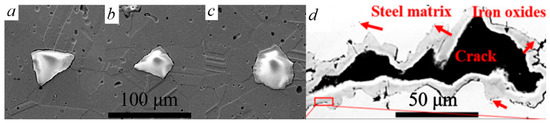
Figure 1.
(a) Triangle-shaped inclusion, (b) quadrilateral-shaped inclusion, (c) polygonal-shaped inclusion [21,22], and (d) macrostructure of the hole, iron oxide, and steel matrix [28].
The aforementioned studies primarily investigated the problems involving only two phases, namely the inclusion and matrix. Moreover, microscopic observation of the Al matrix with SiC [9] or carbon diamond [10] particles and 20NiCr3H steel [28] showed an irregular pore, inclusion, and matrix. Furthermore, the microscopic observation revealed an irregular void, iron inclusion, and steel matrix, as shown in Figure 1d. In addition, an irregular void, inclusion (SiC), and matrix (AlSi7) were detected by Schöbel et al. [9,10]. According to these geometric suggestions, an irregularly shaped hole with a coating layer embedded in the matrix is established, as shown in Figure 2a. A hole can be observed to exist inside and attach to the coating layer embedded in the matrix. In the theoretical model limitation, an “equiangular polygon” is investigated for realizing irregularly shaped inclusion. This composite system, including irregular holes, coating layers, and matrix has been discussed under different conditions [29,30,31,32,33]. However, the previous study [33] can only be utilized to deal with certain triangular or square-coated hole problems under thermal loading. Hence, the general solution of temperature and stress function and singular terms of an irregularly shaped pore with an arbitrary edge and a coating layer are investigated for the first time in this study. Many studies have demonstrated that the majority of materials experience thermal stress (tension or compression) and strain when subjected to different thermal loadings [34,35]. A qualitative and quantitative investigation of thermal stress on the interface is presented in this study.

Figure 2.
The (a) physical plane (z-plane) and (b) mathematical plane (ζ-plane) of a polygonal coated hole under thermal singularity.
In this study, the temperature distribution was solved first with a visualization of the temperature contour. The next step is to determine the proper interfacial stress of a coated pentagonal hole subjected to point thermal singularity. Additionally, parameter analysis is performed, including the shape factor, shear modulus, and thermal expansion coefficient. The remaining of this study is divided into the following sections. Section 2.1 provides the flow diagram of this problem. The general formulation of isotropic thermo-elasticity in two dimensions, as well as mapping techniques, are introduced in Section 2.2. Analytical solutions in the general form of the temperature and interfacial stress of the coated polygonal layer are provided in Section 3.1 and Section 3.2, respectively. The correction terms required to rectify the singular terms are determined using the trial-and-error method in MATLAB, which is described in Section 3.3. In Section 4, practical applications are discussed through a quantitative analysis. Section 5 presents the conclusions.
2. Mathematical Modeling
2.1. Flow Diagram
A flow diagram of the study is shown in Figure 3. The theoretical approach, which comprises the mapping method, analytical continuation, and alternative methodology, is described first. The temperature field is analyzed utilizing theoretical techniques and iterations. To derive the stress function and correction terms, the iterative method and the trial-and-error method are then suggested. The numerical computations, including those for temperature contours and interfacial stresses, are therefore carried out using MATLAB. Finally, output results are acquired and thoroughly analyzed.
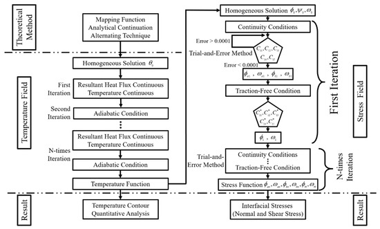
Figure 3.
A flow diagram of the current study including theoretical method, temperature field, stress field, and result.
An analytical solution to the temperature function of the coated polygonal hole can be obtained by using the iterative technique in the temperature field. The homogenous solution of the temperature field is initially introduced. The continuity conditions (temperature and resultant heat flux) are then considered to be satisfied by the outer interface for the first iteration of the temperature field. The inner interface must fulfill the adiabatic condition in order for the second iteration to proceed. It is possible to achieve an analytical solution for the temperature field by repeating the aforementioned iterative techniques until n iterations.
Determining an analytical solution to the stress function in the stress field can be aided by the iterative technique and the trial-and-error method. The homogeneous solution for the stress field is given initially and the unknown solution for the stress field is determined using the analytical continuation theorem. After that, it is ensured that the outer interface should satisfy the continuity conditions (displacement and resultant force) for the first iteration of the stress field. Meanwhile, MATLAB is used to implement a while-loop and the trial-and-error method for determining the correction terms of the outer interface. The traction-free condition is then satisfied by the inner interface and correction terms are applied to derive the stress function of the inner interface. The analytical solution to the stress field can be obtained by repeating the abovementioned iterative steps n times.
The numerical computations are implemented by MATLAB, such as temperature contours and interfacial stresses, after obtaining the analytical solutions for the temperature and stress fields. The final step is undertaking a thorough quantitative and qualitative analysis to compare the output findings and offer reasonable explanations for pertinent practical situations.
2.2. Problem Construction
Figure 1 shows several irregularly shaped inclusions, which must be discussed in detail. To further explore the problem of a coated polygonal hole, we consider an equiangular polygonal hole with a coating layer inlaid with an infinite plane that is subjected to point thermal singularity. The general solution of correction terms and temperature and stress fields are described in this study. Consider that the substrate and coating layer are assumed to be perfectly bonded across the interface . The interface shown in Figure 2a between the coating layer and the hole must satisfy the adiabatic and traction-free conditions in temperature and stress fields, respectively. The two undetermined stress functions () are utilized to determine the displacement and the resultant force. Assume that is the undetermined temperature function. The relevant formula of isotropic thermo-elasticity in two-dimension is given as follows [15,36].
For plane strain deformation, and is considered. The parameters , , and denote the shear modulus, Poisson’s ratio and the coefficient of thermal expansion, respectively. Additionally, the function represents the complex conjugate, and the prime sign implies the derivative associated with . To address the current problem, the mapping function is implemented as follows [15]:
After using the mapping function, the coated polygonal hole in the physical plane (see Figure 2a) with two interfaces and maps onto the concentric circles consisting of two interfaces and in mathematical plane (see Figure 2b). The inside and outside radii of the concentric circles are set to be unity and , respectively in the , as shown in Figure 2b. Assume that and respectively represents the substrate the coating layer with the interface after the transformation. The interface shown in Figure 2b is between the coating layer and a unit circular hole. Moreover, the parameter describes the number of edges on the coated polygonal hole in Equation (3). For example, denotes a triangle; denotes a square, and denotes a pentagon.
Additionally, the magnification factor in Equation (3) is related to particle size. Although “particle size” is being conducted by many researchers [37,38], the parameter was assumed to be unity in this study to simplify the complicated geometry. Another parameter in Equation (3) that might affect the sharpness of polygon corners is the shape factor . The different shape factors of a pentagonal hole () with a coating layer are illustrated in Figure 4. Generally, the edge of the pentagonal hole becomes sharper when is larger. However, the range of the shape factors is defined in Equation (3). The parameter ranges between 0 to . When , the polygonal problem will develop into a hypocycloidal crack. Hence, this study only discusses the range of to avoid singularity with .
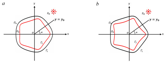
Figure 4.
The different shape factors of a pentagonal coated hole in the physical plane, where (a) w = 0.07 and (b) w = 0.1.
After applying the mapping function, Equations (1) and (2) can be transferred to mathematical plane form, rewritten as follows:
3. Mathematical Formulation
3.1. Temperature Field
Consider that the temperature function fulfills the homogeneous differential equation (Laplace equation) of the steady-state heat conduction problem [36]. The complex potential is related to temperature and heat flux as
where Re and Im respectively represent the real and imaginary parts in Equations (6) and (7). The components and in Equation (7) are the x and y- directions of the heat flux, respectively. The parameter is the coefficient of the heat conductivity.
The homogeneous solution of the temperature field subject to point thermal singularity in an infinite substrate is written as follows [36]
where (or ) is defined as a point heat source (or a point heat sink); and are the strength and position of the point thermal singularity, respectively. The temperature functions of a coated hole under a point thermal singularity are assumed as
where is holomorphic in region (); and are both holomorphic in region ().
Using the analytical continuation and alternation method, the temperature functions in Equation (9) can be obtained in terms of as
where
Integration of Equation (10) with yields:
where the temperature functions and are holomorphic in the region ; and , are holomorphic in region . It should be noted that the solutions in Equation (17) are the series solution for arbitrarily shaped coated polygonal holes. The temperature functions , , , and in Equations (13) are respectively derived in Appendix A.
3.2. Stress Field
To facilitate the derivation of boundary conditions, an auxiliary stress function is introduced as
In order to satisfy the single-valued conditions of displacement and resultant force, Equations (4) and (5), the stress functions of the present problem must be formulated as follows:
where and are holomorphic in region (); , , , and are holomorphic in regions ().
The general expressions of M and N for different values of are given by:
First, the stress functions at the interface must satisfy the continuity conditions. The general form of the first analytical continuation at interface yields:
where
the interface between the coating layer and the hole must fulfill the traction-free condition. The general form of the second analytical continuation at interface yields:
where
Third, returning to the stress functions at the interface , they must satisfy the continuity conditions at the interface . The general solution of the third analytical continuation at interface yields:
where
After repeating the analytical continuation in association with the alternation method, the remaining stress functions are determined as;
where
3.3. Trial-and-Error Method
After the mathematical solution is obtained, the numerical calculation is implemented using MATLAB. The most difficult part of exporting numerical results is dealing with correction terms that appear in the stress field. According to the flow diagram (see Figure 3), the zero iteration for the stress field is the homogeneous solution and . The first iteration happens on interface
, where the stress functions are , and . The continuity conditions (displacement and resultant force continuous) must satisfy along the interface . However, and are mutually dependent functions, which means the correction term cannot be determined directly. Hence, the trial-and-error method is used to obtain the correction term. A discriminant equation is introduced initially and expressed as follows;
where and respectively represent the initial and final values of the correction term , and is the absolute difference between and . The detailed iterative process is as follows:
First, the term can be derived by substituting into Equation (19). Next, can be obtained by substituting into Equation (27). After the terms of and are determined, the difference between and could be calculated as displayed in Equation (33). Based on the while-loop, the iteration continued or stopped when is larger or less than 0.0001, respectively. The value replaces the value when the difference is larger than 0.0001, as shown in Equation (34). Then, the new term could be derived by substituting the replaced term into Equation (19) again. Simultaneously, could be yielded by substituting . After that, the status of the iteration depends on the difference between and as displayed in Equation (33). Conversely, the iteration could be forcibly terminated because of the convergent value for when the difference value is less than 0.0001, as shown in Equation (35). Herein, the latest value of would be defined as the approximate correction term . Finally, the actual stress function could be solved when the approximate correction term is confirmed.
Because of the traction-free condition, the additional terms and must be satisfied along the interface . . The correction term for the interface could be determined directly because involves as shown in Equation (24), where is yielded by the differential of the latest obtained term in the first iteration for the interface . The approximate correction term is derived by substituting the term into Equation (24). Lastly, the actual stress function could be solved by substituting the approximate correction term into Equation (22).
The second iteration for the interface is considered after the stress function is determined. The continuity conditions of displacement and resultant force must be satisfied by the stress functions , and along the interface . A discriminant equation of the second iteration for the interface is represented as follows:
where and respectively represent the initial and final values of the correction term , and is the absolute difference between and . The detailed iterative process is as follows:
Similar to the first iteration, the term could be calculated by substituting into Equation (25). Meanwhile, can be yielded by substituting into Equation (28). Next, is calculated after the terms of and are determined, as displayed in Equation (36). The iteration continues or stops when is larger or less than 0.0001, respectively, as described in Equations (37) and (38). Then, the approximate correction term is derived when the iteration stops. After that, the actual stress function for the interface could be determined by substituting the approximate correction term , which is yielded by substituting the latest obtained term of . Finally, the general rules of the iteration for the polygonal hole with a coating layer could be summarized based on the above skill until n-times iteration.
A general form of the discriminant equation for the n-times iteration is written as:
where is the difference value; and are the initial and final values of the correction terms in the corresponding situation, respectively.
By following the rules mentioned in this section, a series of correction terms could be determined.
4. Numerical Results
4.1. Temperature Distribution
The general form of temperature potential of a coated polygonal hole subjected to point thermal singularity is expressed in Equation (13). The temperature field for a coated triangle, square, and pentagonal hole with under a point thermal singularity located at (3,0) and (−3,0) is considered in this study. Figure 5, Figure 6 and Figure 7a,b show the isothermal contours for a coated equiangular polygonal hole with different ratios of thermal conductivity. Furthermore, Figure 5, Figure 6 and Figure 7c show the quantitative analysis of a coated polygonal hole with different thermal conductivities.
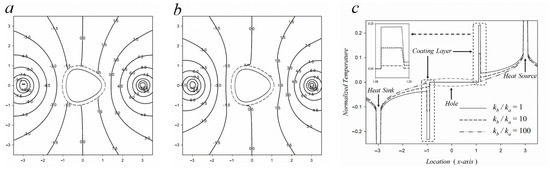
Figure 5.
Contours of temperature distribution for a coated equiangular triangle hole, where (a) kb/ka = 10 and (b) kb/ka = 100. (c) Quantitatively normalized temperature for a coated triangular hole with different ratios of heat conductivity, where w = 0.1.
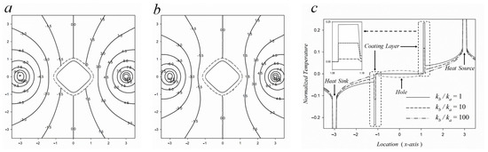
Figure 6.
Contours of temperature distribution for a coated equiangular square hole, where (a) kb/ka = 10 and (b) kb/ka = 100. (c) Quantitatively normalized temperature for a coated triangular hole with different ratios of heat conductivity, where w = 0.1.
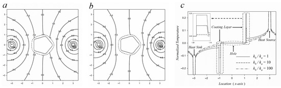
Figure 7.
Contours of temperature distribution for a coated equiangular pentagonal hole, where (a) kb/ka = 10 and (b) kb/ka = 100. (c) Quantitatively normalized temperature for a coated triangular hole with different ratios of heat conductivity, where w = 0.1.
Figure 5, Figure 6 and Figure 7a,b show the temperature contour distribution for different ratios of thermal conductivity. It can be pointed out that the isothermal contours have different changes in different ratios of thermal conductivity with and . When the thermal conductivity of the coating layer is increased, the contour lines around the coated hole are more dispersed. On the contrary, when the thermal conductivity of the coating layer is decreased, the contour lines around the coated hole are concentrated. It means that the higher thermal conductivity of the coating layer has a better heat dissipation effect. That is, a higher thermal conductivity can avoid a larger temperature gradient and prevent damage to the material at high temperatures. This phenomenon can be observed in the case of , which can be seen from Figure 5, Figure 6 and Figure 7b.
The previously proposed isothermal contours belong to qualitative analysis that is based on personal visual perception. To obtain more accurate temperature results, the following arguments are explored with appropriate quantitative analysis. To discuss the temperature evolution on the x-axis, Figure 5, Figure 6 and Figure 7c provide a quantitative analysis of a coated equiangular triangle, square, and pentagonal hole with different thermal conductivities. For the limiting case of a polygonal hole, , the heat flow is always along the adiabatic hole. It can be discovered that there exists a larger gradient due to which the temperature increases and decreases rapidly around the coating layer. This is because the theoretically adiabatic condition is assumed around the hole. Hence, the temperature is concentrated on the coating layer ((1.1,0) and (−1.1,0)), indicating that temperature approaches zero close to the hole due to adiabatic conditions. Furthermore, it can be evidently observed from the enlarged view in the upper left corner of Figure 5, Figure 6 and Figure 7c that when , the temperature around the hole is 0.24; when , the temperature drops to 0.12, and when , the temperature drops further to near zero. It can be realized that, when the thermal conductivity rises by a factor of 10, the temperature can be reduced by half. The reason for this phenomenon is that the coating layer with a high thermal conductivity has the effect of heat absorption. This shows that when thermal conductivity is larger, the effect of endothermic is more obvious. The same trend can be seen from the different shaped coated holes in Figure 5, Figure 6 and Figure 7c.
When the entire material containing a coating layer is in a high-temperature environment, the coating layer with a higher thermal conductivity could display a lower temperature gradient environment. Herein, it will not be damaged in harsh temperature conditions, and the coating layer can achieve the effect of protecting the irregularly shaped holes and substrate. Furthermore, materials with higher thermal conductivity should be chosen because they can resist thermal fatigue and also have good heat absorption [10].
4.2. Interfacial Stresses
The summarized general stress functions of a coated equiangular polygonal hole applied to a point thermal singularity are given in Equations (29) and (30). In this study, all the results of stress fields are based on a coated pentagonal hole; that is, in Equation (5). In this section, we discuss a parametric analysis for point thermal singularity, shear modulus, thermal expansion coefficient, and shape factor.
Figure 8 shows a parametric analysis of different strengths of point thermal singularity for the coated pentagonal hole. A point heat source or sink was assumed to be located at point (3,0) along the x-axis. As predicted, when the strength of a point thermal singularity is high, the interfacial stress is increased. In Figure 8, the two curves at the bottom represent point heat source. The point heat source causes a compressive normal stress at the interface because the coating layer expands at high temperatures and the substrate resists it. Conversely, the two curves at the top represent the point heat sink. Tensile normal stress appears at the interface because the coating layer shrinks at low temperatures and the substrate invades it. The interfacial normal stress of each corner of the pentagonal hole under different magnitudes of heat loading is shown in Table 1. The interfacial stress has a positive and negative value under heat sink and source, respectively. The interfacial stress reduces by half as the magnitude of the thermal loading decreases by half. This can provide a reasonable explanation of the void evolution in MMC during the cooling stage. Both Al matrix with carbon diamond and AlSi7 matrix with SiC particle composites [10] exhibit the formation of irregularly shaped voids along the interface at eutectic solidification. Small rounded pores were observed to have formed within the SiC particles owing to the shrinkage of aluminum at the eutectic solidification. Subsequently, the small pores coalesced into larger irregular pores during the cooling stage [10]. Larger voids are generated because higher interfacial tensile stress occurs between the coating and adjacent materials when the temperature drops.
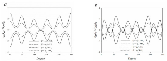
Figure 8.
Interfacial (a) normal and (b) shear stress of a coated pentagonal hole (w = 0.05, Gb/Ga = 3, βb/βb = 3, kb/ka = 2, νb = 0.3, νa = 0.3).

Table 1.
The interfacial normal stress of each corner of the pentagonal hole under different magnitudes of heat loading.
The interfacial normal and shear stresses for a pentagonal coated hole subjected to a point heat source is respectively symmetric and anti-symmetric with respect to the x-axis, as shown in Figure 9, Figure 10 and Figure 11, and this trend is similar to those reported in a previous study [33]. The extreme values of interfacial normal stress occurred at the corners of a pentagonal coating layer (0°, 72°, 144°, 216°, and 288°). In contrast, the interfacial shear stress vanishes at the corners of a pentagonal coating layer (0°, 72°, 144°, 216°, and 288°). Table 2 presents the interfacial normal stress of each corner of the pentagonal hole with different parameters. Table 2 depicts that the interfacial normal stress exhibited a maximum value as the corner was 0°. The corner 0° of a coated pentagonal hole was closer to the point heat source, which implies that a larger temperature gradient exists. Therefore, the interfacial normal stress was larger. Conversely, interfacial normal stress was smaller when the corner was 144° and 216°, which are far away from the point heat source.
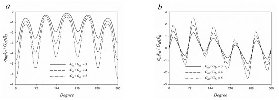
Figure 9.
Interfacial (a) normal and (b) shear stress of a coated pentagonal hole (w = 0.05, βb/βb = 3, kb/ka = 2, νb = 0.3, νa = 0.3).
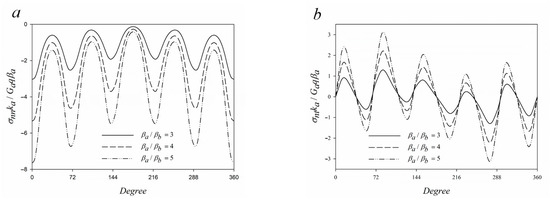
Figure 10.
Interfacial (a) normal and (b) shear stress of a coated pentagonal hole (w = 0.05, Gb/Ga = 3, kb/ka = 2, νb = 0.3, νa = 0.3).
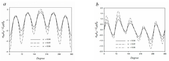
Figure 11.
Interfacial (a) normal and (b) shear stress of a coated pentagonal hole (Gb/Ga = 3, βb/βb = 3, kb/ka = 2, νb = 0.3, νa = 0.3).
Table 2.
The interfacial normal stress of each corner of the pentagonal hole with different parameters.
Figure 9 expresses the interfacial stresses with different shear modulus ratios of a coated pentagonal hole subjected to a point heat source. Evidently, the interfacial stresses increased with a larger shear modulus of the coating layer. Previous research [39] reported that different modulus ratios of the coatings cause “elastic mismatch” and act as an important factor in controlling failure modes. In fracture mechanics, the interfacial delamination results from an increase in driving force when the elastic mismatch increases. The effect of different thermal expansion coefficient ratios around a coated pentagonal hole is shown in Figure 10. Due to different thermal expansion coefficients of the coating layer and the substrate, a phenomenon known as “thermal mismatch” occurs during the cooling phase. In addition, the interface between the substrate and coating layer may easily fracture due to the increased tensile stress caused by the thermal mismatch. Furthermore, Table 2 and Figure 9 and Figure 10 present that the interfacial stress is dominated by the thermal expansion coefficient compared to the shear modulus. Figure 11 presents the interfacial stress around a coated pentagonal hole with different shape factors. The interfacial stress around the coating layer was observed to be more intensified when the shape factor was larger. When the shape factor is large, the coating layer becomes sharper, and serious stress concentration is likely to occur at the corners of the interface. For practical engineering applications, the debonding mechanism is likely to result in interfacial failure due to interfacial stress concentration at the corners of the composites [40]. In addition, for TRIP-steel of MMC, the point of ductile damage begins from the sharper corners of the interface of the austenite matrix and zirconia particle when the global strain increases. However, most of the zirconia particles were cracked, void coalescence began to appear, and the damage progressed faster when the stress reached a critical value [41].
5. Conclusions
A general solution for a polygonal hole with a coating layer located at an infinite substrate under point thermal singularity is investigated in this study. A rapidly convergent series solution of both temperature and stress functions is obtained in an elegant form for the composites problem of an irregularly shaped void, inclusion, and substrate on the premise of using the conformal mapping function, analytical continuation theorem, and alternation method. The correction terms, expressed as a general solution, are solved using the trial-and-error method in MATLAB. The general solution proposed in this study is applied to the case with any number of edges of the polygonal hole with the coating layer. As numerical examples, the distribution of temperature contours provides the best optimal design with high thermal conductivity of the coating layer, thereby resulting in better heat absorption capacity through quantitative analysis. The interfacial stress demonstrated a larger stress concentration that occurred at the corners of the coated polygonal pores under thermal loading. Moreover, a reasonable explanation is provided for the growth of irregular voids in MMC during the cooling stage.
Author Contributions
Conceptualization: C.-K.C. and Y.-L.L.; methodology, Y.-L.L. and C.-K.C.; software, Y.-L.L. and S.-C.T.; formal analysis, Y.-L.L. and S.-C.T.; investigation, Y.-L.L.; resources, S.-C.T.; data curation, Y.-L.L. and S.-C.T.; writing—original draft preparation, Y.-L.L. and S.-C.T.; writing—review and editing, C.-K.C. and S.-C.T.; visualization, Y.-L.L. and S.-C.T.; project administration, C.-K.C. All authors have read and agreed to the published version of the manuscript.
Funding
This research was supported by the Ministry of Science and Technology of Taiwan under the grant MOST 106-2221-E-011-065-MY3.
Institutional Review Board Statement
Not applicable.
Informed Consent Statement
Not applicable.
Data Availability Statement
The data presented in this study are available on request from the corresponding author after obtaining permission from the authorized individual.
Acknowledgments
The authors acknowledge the support of Markus Kirschner and Heiko Winderlich (IMF, Technische Universität Bergakademie Freiberg) help regarding the capture microstructure of TRIP-steel with Mg-PSZ.
Conflicts of Interest
The authors declare no conflict of interest.
Appendix A. Determination of M and N in Equations (19) and (20)
Appendix A.1. For the Case of a Triangular Hole Where
The temperature function can be divided into three parts:
where and are defined as
The constant A in (A1) is defined as
The displacement can be expressed as
This leads to
where . The coefficient of the logarithmic term must vanish, which yields
Solving for M in Equation (A5) yields
The temperature potential function must be split into three parts:
where and are defined as
And the constant B in (A7) is defined as
The displacement can be expressed as
which leads to
Substituting (A8) into (A10), we obtain
Appendix A.2. For the Case of a Square Hole Where
The temperature function of are shown below
The constants M and N for yield
Appendix A.3. For the Case of a Pentagonal Hole Where
The temperature function of are shown below
The constants M and N for yield
References
- Zweben, C. Metal-matrix composites for electronic packaging. J. Miner. Met. Mater. Soc. 1992, 44, 15–23. [Google Scholar] [CrossRef]
- Beffort, O.; Vaucher, S.; Khalid, F. On the thermal and chemical stability of diamond during processing of Al/diamond composites by liquid metal infiltration (squeeze casting). Diam. Relat. Mater. 2004, 13, 1834–1843. [Google Scholar] [CrossRef]
- Jagadeesh, G.V.; Setti, S.G. A review on micromechanical methods for evaluation of mechanical behavior of particulate reinforced metal matrix composites. J. Mater. Sci. 2020, 55, 9848–9882. [Google Scholar] [CrossRef]
- Hussein, T.; Umar, M.; Qayyum, F.; Guk, S.; Prahl, U. Micromechanical Effect of Martensite Attributes on Forming Limits of Dual-Phase Steels Investigated by Crystal Plasticity-Based Numerical Simulations. Crystals 2022, 12, 155. [Google Scholar] [CrossRef]
- Qayyum, F.; Umar, M.; Guk, S.; Schmidtchen, M.; Kawalla, R.; Prahl, U. Effect of the 3rd Dimension within the Representative Volume Element (RVE) on Damage Initiation and Propagation during Full-Phase Numerical Simulations of Single and Multi-Phase Steels. Materials 2020, 14, 42. [Google Scholar] [CrossRef]
- Schöbel, M.; Degischer, H.; Vaucher, S.; Hofmann, M.; Cloetens, P. Reinforcement architectures and thermal fatigue in diamond particle-reinforced aluminum. Acta Mater. 2010, 58, 6421–6430. [Google Scholar] [CrossRef]
- Nam, T.H.; Requena, G.; Degischer, P. Thermal expansion behaviour of aluminum matrix composites with densely packed SiC particles. Compos. Part A Appl. Sci. Manuf. 2008, 39, 856–865. [Google Scholar] [CrossRef]
- Beffort, O.; Khalid, F.; Weber, L.; Ruch, P.; Klotz, U.; Meier, S.; Kleiner, S. Interface formation in infiltrated Al(Si)/diamond composites. Diam. Relat. Mater. 2006, 15, 1250–1260. [Google Scholar] [CrossRef]
- Schöbel, M.; Altendorfer, W.; Degischer, H.; Vaucher, S.; Buslaps, T.; Di Michiel, M.; Hofmann, M. Internal stresses and voids in SiC particle reinforced aluminum composites for heat sink applications. Compos. Sci. Technol. 2011, 71, 724–733. [Google Scholar] [CrossRef]
- Schöbel, M.; Requena, G.; Fiedler, G.; Tolnai, D.; Vaucher, S.; Degischer, H. Void formation in metal matrix composites by solidification and shrinkage of an AlSi7 matrix between densely packed particles. Compos. Part A Appl. Sci. Manuf. 2014, 66, 103–108. [Google Scholar] [CrossRef]
- Rivera-Salinas, J.E.; Gregorio-Jáuregui, K.M.; Romero-Serrano, J.A.; Cruz-Ramírez, A.; Hernández-Hernández, E.; Miranda-Pérez, A.; Gutierréz-Pérez, V.H. Simulation on the Effect of Porosity in the Elastic Modulus of SiC Particle Reinforced Al Matrix Composites. Metals 2020, 10, 391. [Google Scholar] [CrossRef]
- Evans, A.G.; Mumm, D.R.; Hutchinson, J.W.; Meier, G.H.; Pettit, F.S. Mechanisms controlling the durability of thermal barrier coatings. Prog. Mater. Sci. 2001, 46, 505–553. [Google Scholar] [CrossRef]
- Ramakrishnan, N.; Arunachalam, V.S. Effective elastic moduli of porous solids. J. Mater. Sci. 1990, 25, 3930–3937. [Google Scholar] [CrossRef]
- Ramakrishnan, N.; Arunachalam, V.S. Effective Elastic Moduli of Porous Ceramic Materials. J. Am. Ceram. Soc. 1993, 76, 2745–2752. [Google Scholar] [CrossRef]
- Muskhelishvili, N.I. Some Basic Problems of the Mathematical Theory of Elasticity; Noordhoff: Groningen, The Netherlands, 1953; Volume 15. [Google Scholar] [CrossRef]
- Chao, C.K.; Chen, F.M.; Shen, M.H. Green’s Functions for a Point Heat Source in Circularly Cylindrical Layered Media. J. Therm. Stress. 2006, 29, 809–847. [Google Scholar] [CrossRef]
- Chao, C.; Chen, F.; Lin, T. Green’s function for a point heat source embedded in an infinite body with two circular elastic inclusions. Appl. Math. Model. 2018, 56, 254–274. [Google Scholar] [CrossRef]
- Chao, C.K.; Chen, C.K.; Chen, F.M. Interfacial stresses induced by a point heat source in an isotropic plate with a reinforced elliptical hole. Comput. Model. Eng. Sci. (CMES) 2010, 63, 1. [Google Scholar] [CrossRef]
- Zenkour, A.M.; Mashat, D.S.; Allehaibi, A.M. Thermoelastic Coupling Response of an Unbounded Solid with a Cylindrical Cavity Due to a Moving Heat Source. Mathematics 2022, 10, 9. [Google Scholar] [CrossRef]
- Attia, M.A.; Melaibari, A.; Shanab, R.A.; Eltaher, M.A. Dynamic Analysis of Sigmoid Bidirectional FG Microbeams under Moving Load and Thermal Load: Analytical Laplace Solution. Mathematics 2022, 10, 4797. [Google Scholar] [CrossRef]
- Chiu, C.; Tseng, S.; Qayyum, F.; Guk, S.; Chao, C.; Prahl, U. Local deformation and interfacial damage behavior of partially stabilized zirconia-reinforced metastable austenitic steel composites: Numerical simulation and validation. Mater. Des. 2022, 225, 111515. [Google Scholar] [CrossRef]
- Tseng, S.-C.; Chiu, C.-C.; Qayyum, F.; Guk, S.; Chao, C.-K.; Prahl, U. The Effect of the Energy Release Rate on the Local Damage Evolution in TRIP Steel Composite Reinforced with Zirconia Particles. Materials 2023, 16, 134. [Google Scholar] [CrossRef] [PubMed]
- Xie, C.; Wu, Y.; Liu, Z. Stress fields and effective modulus of piezoelectric fiber composite with arbitrary shaped inclusion under in-plane mechanical and anti-plane electric loadings. Math. Mech. Solids 2019, 24, 3180–3199. [Google Scholar] [CrossRef]
- Luo, J.-C.; Gao, C.-F. Stress field of a coated arbitrary shape inclusion. Meccanica 2011, 46, 1055–1071. [Google Scholar] [CrossRef]
- Yoshikawa, K.; Hasebe, N. Green’s function of the displacement boundary value problem for a heat source in an infinite plane with an arbitrary shaped rigid inclusion. Arch. Appl. Mech. 1999, 69, 227–239. [Google Scholar] [CrossRef]
- Tang, J.-Y.; Yang, H.-B. An alternative numerical scheme for calculating the thermal stresses around an inclusion of arbitrary shape in an elastic plane under uniform remote in-plane heat flux. Acta Mech. 2019, 230, 2399–2412. [Google Scholar] [CrossRef]
- Yang, Q.; Zhu, W.; Li, Y.; Zhang, H. Stress field of a functionally graded coated inclusion of arbitrary shape. Acta Mech. 2018, 229, 1687–1701. [Google Scholar] [CrossRef]
- Zhou, X.; Shao, Z.; Tian, F.; Hopper, C.; Jiang, J. Microstructural effects on central crack formation in hot cross-wedge-rolled high-strength steel parts. J. Mater. Sci. 2020, 55, 9608–9622. [Google Scholar] [CrossRef]
- Tseng, S.C.; Chao, C.K.; Chen, F.M. Interfacial Stresses of a Coated Square Hole Induced by a Remote Uniform Heat Flow. Int. J. Appl. Mech. 2020, 12, 2050063. [Google Scholar] [CrossRef]
- Tseng, S.C.; Chao, C.K.; Guo, J.Y. Failure Analysis of a Polygonal Void with an Oxide Layer in a Cracked Matrix. Int. J. Appl. Mech. 2021, 13, 2150099. [Google Scholar] [CrossRef]
- Chiu, C.; Tseng, S.; Chao, C.; Guo, J. Stress Intensity Factors for a Non-Circular Hole with Inclusion Layer Embedded in a Cracked Matrix. Aerospace 2021, 9, 17. [Google Scholar] [CrossRef]
- Liao, Y.L.; Tseng, S.C.; Chao, C.K. Stress analysis of an inclusion layer bonded to an irregularly shaped pore under an edge dislocation or a concentrated load. J. Mech. 2022, 38, 397–409. [Google Scholar] [CrossRef]
- Tseng, S.C.; Chao, C.K.; Chen, F.M.; Chiu, W.C. Interfacial stresses of a coated polygonal hole subject to a point heat source. J. Therm. Stress. 2020, 43, 1487–1512. [Google Scholar] [CrossRef]
- Xue, X.-Y.; Wen, S.-R.; Sun, J.-Y.; He, X.-T. One- and Two-Dimensional Analytical Solutions of Thermal Stress for Bimodular Functionally Graded Beams under Arbitrary Temperature Rise Modes. Mathematics 2022, 10, 1756. [Google Scholar] [CrossRef]
- He, X.-T.; Zhang, M.-Q.; Pang, B.; Sun, J.-Y. Solution of the Thermoelastic Problem for a Two-Dimensional Curved Beam with Bimodular Effects. Mathematics 2022, 10, 3002. [Google Scholar] [CrossRef]
- Bogdanoff, J.L. Note on Thermal Stresses. J. Appl. Mech. 1954, 21, 88. [Google Scholar] [CrossRef]
- Qayyum, F.; Chaudhry, A.A.; Guk, S.; Schmidtchen, M.; Kawalla, R.; Prahl, U. Effect of 3D Representative Volume Element (RVE) Thickness on Stress and Strain Partitioning in Crystal Plasticity Simulations of Multi-Phase Materials. Crystals 2020, 10, 944. [Google Scholar] [CrossRef]
- Wu, C.; Wang, D.; Guo, Y. An immersed particle modeling technique for the three-dimensional large strain simulation of particulate-reinforced metal-matrix composites. Appl. Math. Model. 2016, 40, 2500–2513. [Google Scholar] [CrossRef]
- Jiang, P.; Fan, X.; Sun, Y.; Li, D.; Li, B.; Wang, T. Competition mechanism of interfacial cracks in thermal barrier coating system. Mater. Des. 2017, 132, 559–566. [Google Scholar] [CrossRef]
- Evans, A.G.; He, M.Y.; Hutchinson, J.W. Mechanics-based scaling laws for the durability of thermal barrier coatings. Prog. Mater. Sci. 2001, 46, 249–271. [Google Scholar] [CrossRef]
- Qayyum, F.; Guk, S.; Prahl, U. Studying the Damage Evolution and the Micro-Mechanical Response of X8CrMnNi16-6-6 TRIP Steel Matrix and 10% Zirconia Particle Composite Using a Calibrated Physics and Crystal-Plasticity-Based Numerical Simulation Model. Crystals 2021, 11, 759. [Google Scholar] [CrossRef]
Disclaimer/Publisher’s Note: The statements, opinions and data contained in all publications are solely those of the individual author(s) and contributor(s) and not of MDPI and/or the editor(s). MDPI and/or the editor(s) disclaim responsibility for any injury to people or property resulting from any ideas, methods, instructions or products referred to in the content. |
© 2023 by the authors. Licensee MDPI, Basel, Switzerland. This article is an open access article distributed under the terms and conditions of the Creative Commons Attribution (CC BY) license (https://creativecommons.org/licenses/by/4.0/).