Credibilistic Cournot Game with Risk Aversion under a Fuzzy Environment

Abstract

The classic Cournot game ignores the influence of the players’ psychological behavior on the decision and cannot deal with the game problem of fuzzy information. To address such game situations, a credibilistic Cournot game is developed, where the optimistic value criterion derived from credibility theory is used to describe risk-averse behavior of manufacturers and the associated parameters are characterized by fuzzy variables. Then, a concept of the (α₁, α₂)-optimistic equilibrium quantity is proposed and its uniqueness is shown. Finally, the relevant results of the credibilistic Cournot game are applied to an example to illustrate the availability of our model, and a sensitivity analysis of the relationship between the (α₁, α₂)-optimistic equilibrium quantity and confidence levels is performed. The results show that manufacturers’ (α₁, α₂)-optimistic equilibrium quantity is positively related to the risk aversion level of their competitors and negatively to their own risk aversion level.

1. Introduction

As a common market mechanism, an oligopoly market refers to the market structure in which a certain industry is completely controlled by a few manufacturers. The classic Cournot game model is used to study the equilibrium quantity problem of a duopoly industry. However, the application of the classical Cournot game model in practical problems is often limited by many uncertain factors (such as consumer demand or production fluctuations). For example, the outbreak of COVID-19 in 2019 made the home office a normal situation, leading to a surge in demand for electronic products such as PCs and smart phones. Although manufacturers worked overtime to purchase components and expand production, the supply of products still was not adequate for demand, and delayed delivery became a problem faced by many enterprises (https://www.chinatimes.com/cn/realtimenews/20201226004090260410?chdtv accessed on 26 December 2020). After 2022, the demand for PCs, smart phones, and other electronic products slowed, resulting in a glut of products (https://www.expreview.c-om/83750.html accessed on 25 December 2022). The classical Cournot game fails to approach to such situations with uncertain information. Therefore, the Cournot game under uncertain scenarios has received extensive attention.

To address such uncertainties, Zadeh proposed the concept of a fuzzy set in 1965 [1]. Some scholars combined the Cournot model with fuzzy set theory and proposed a kind of Cournot game model with fuzzy parameters. Yao and Wu [2] applied the sorting method to change the fuzzy numbers in the supply and demand function into real numbers to calculate the consumer surplus and producer surplus. Wu and Yao [3] constructed the inventory model based on [2]. Ouyang and Yao [4] studied the inventory model based on the demand function with triangular fuzzy numbers and statistical fuzzy numbers. Yao and Wu [5] studied the optimal prices of two complementary commodities in a fuzzy environment. Yao and Chang [6] obtained the optimal output by using a fuzzy profit function whose parameters were fuzzy numbers. Yao and Shih [7] obtained the membership function of the profit function based on the optimal production. Xu and Zhai [8] proposed an optimization scheme based on fuzzy set theory to solve the uncertainty problem of demand in the supply chain. Liang et al. [9] constructed the Cournot model based on fuzzy cost to obtain the optimal production of each enterprise. Wang et al. [10] proposed a fuzzy Bayesian game based on credibility theory. Dang and Hong [11] ensured that the equilibrium quantity is positive by strict definition and constructed the Cournot model through a control mechanism. Dang et al. [12] constructed the Cournot game of multiple manufacturers in a competitive market under a fuzzy environment and provided the solution steps for each manufacturer’s equilibrium quantity. Tan et al. [13] discussed the Cournot game with asymmetric information under a fuzzy environment based on the hierarchical dependent utility theory. The differences between this paper and existing literatures are shown in

Table 1. Summary of literature.

Relevant Literature	Fuzzy Supply	Fuzzy Demand	Fuzzy Price	Fuzzy Cost	Credibility Theory	Hierarchical Dependent Utility	Risk Aversion
Yao and Wu [2]; Wu and Yao [3]	√	√
Ouyang and Yao [4]; Yao and Wu [5] Yao and Shih [7]; Xu and Zhai [8]		√
Yao and Chang [6]; Dang and Hong [11] Dang et al. [12]		√	√	√
Liang et al. [9]				√
Wang et al. [10]		√	√		√
Tan et al. [13]		√	√	√		√
Our work		√	√	√	√		√

.

It is worth noting that the extant literature on the Cournot game with fuzzy parameters mainly focuses on “perfect rationality”. However, in real-game problems, players tend to show the behavior characteristic of “limited rationality”, including loss aversion [14,15,16,17], risk aversion [18,19], altruistic and spiteful preferences [20,21], and reference-dependent preferences [22,23,24]. In particular, when faced with gains, people tend to show risk aversion instead of seeking to maximize their gains. Risk aversion has received attention extensively in the classical non-cooperative game [25,26,27], while it has received little attention in the fuzzy environment. In the fuzzy environment, the optimistic value criterion derived from credibility theory is often used to describe the behavior of decision makers [28,29]. The decision makers are risk-averse and want to maximize the optimistic value of their own payoffs for a given confidence level. The confidence levels reflect the risk aversion levels of the decision makers [28]. Since Gao et al. applied credibility theory to solve the matrix game problem with fuzzy payment, risk aversion has received attention in the fuzzy game [28,29,30].

An interesting observation is that the existing literature on the fuzzy game with credibility theory mainly focuses on the fuzzy matrix and bimatrix games with rational preferences and loss aversion [31], but the fuzzy games with risk aversion have received little attention, especially the Cournot game. In real-game situations, players usually show risk aversion. For example, Samsung and Apple have all reduced their planned smart phones in 2023 to avoid the risk of demand reduction (https://www.chinanews.com.cn/cj/2022/11-11/9891967.shtml accessed on 11 November 2022). Another example of risk aversion for firms is in the PC industry, such as HP’s and Lenovo’s reduction in PC production (https://www.jiemian.com/article/8440198.html accessed on 22 November 2022). Therefore, it is essential to explore the influence of risk aversion on decisions for a Cournot game under an uncertain environment. Our work focuses on a Cournot game with risk aversion, where the optimistic value criterion derived from credibility theory is used to characterize players’ behaviors of risk aversion. The influences of risk aversion on equilibrium quantity and market-clearing price are discussed.

The arrangement of this paper is as follows. Section 2 briefly reviews credibility theory. Section 3 constructs the credibilistic Cournot game model and defines the concept of the (α₁, α₂)-optimistic equilibrium quantity, whose uniqueness is shown. A case analysis is shown in Section 4. In Section 5, the conclusions are shown.

2. Credibility Theory

Credibility theory [32,33] is often used to describe the decision behavior of decision makers in a fuzzy environment and is widely used in many fields, such as transportation planning, portfolio selection, and so on.

Definition 1

([33]). Let $\mathsf{\Theta }$ be the non-empty set and let $\mathsf{\Xi }(\mathsf{\Theta })$ be the power set of $\mathsf{\Theta }$. Then Cr{·} is the credibility measure if the following axioms are satisfied.

Axiom 1. Cr{$\mathsf{\Theta }$} = 1;

Axiom 2. Cr{A} $\le$ Cr{B}, where A $\subset$ B;

Axiom 3. Cr{A} + Cr{A^c} = 1, where $A\in \mathsf{\Xi }(\mathsf{\Theta })$;

Axiom 4. Cr{∪_i Ai} = sup_iCr{ A_i}, for any {A_i} with sup_iCr{A_i} < 0.5.

Definition 2

([33]). The triple $(\mathsf{\Theta },\mathsf{\Xi }(\mathsf{\Theta }),Cr)$ is called the credibility space.

Definition 3

([33]). A fuzzy variable $\tilde{\xi }$ is a measurable function from a credibility space $(\mathsf{\Theta },\mathsf{\Xi }(\mathsf{\Theta }),Cr)$ to the set of real numbers.

Lemma 1

([33]). If $\tilde{\xi }$ is a fuzzy variable and its membership function is $\mu$, then for real set R, the credibility measure is

$$Cr\{\tilde{\xi }\in R\}=\frac{1}{2}\underset{x\in R}{(\sup }\mu (x)+1-\underset{x\notin R}{\sup }\mu (x))$$

(1)

Even if the possibility of a fuzzy event reaches one, it may still fail, and even though its necessity is zero, it may still occur. Nevertheless, the fuzzy event must occur if its possibility is equal to one and fail if its credibility is equal to zero [34].

As a special class of fuzzy variables, the triangular fuzzy numbers are denoted as $\tilde{\xi }=({\xi }_l,{\xi }_m,{\xi }_r)$, where ${\xi }_m$ is the median of $\tilde{\xi }$, and ${\xi }_l$ and ${\xi }_r$ are the lower and upper bounds of $\tilde{\xi }$ [35]. Its membership function is

$$\mu (x)=\{\begin{array}{ll}(x-{\xi }_l)/({\xi }_m-{\xi }_l)& \hspace{0.17em}{\xi }_l\le x<{\xi }_m\\ 1& \hspace{0.17em}x={\xi }_m\\ ({\xi }_r-x)/({\xi }_r-{\xi }_m)& \hspace{0.17em}{\xi }_m<x\le {\xi }_r\\ 0& others\end{array}$$

If ${\xi }_l\ge 0, {\xi }_r>0$, $\tilde{\xi }=({\xi }_l,{\xi }_m,{\xi }_r)$ is called the non-negative triangular fuzzy number.

Let $\tilde{\xi }=({\xi }_l,{\xi }_m,{\xi }_r)$ and $\tilde{\eta }=({\eta }_l,{\eta }_m,{\eta }_r)$ be two triangular fuzzy numbers; the operation rules are shown as follows [36].

$$\tilde{\xi }+\tilde{\eta }=({\xi }_l+{\eta }_l,{\xi }_m+{\eta }_m,{\xi }_r+{\eta }_r)$$

(2)

$$\lambda \tilde{\xi }=(\lambda {\xi }_l,\lambda {\xi }_m,\lambda {\xi }_r)\lambda \ge 0.$$

(3)

$$\tilde{\xi }-\tilde{\eta }=({\xi }_l-{\eta }_r,{\xi }_m-{\eta }_m,{\xi }_r-{\eta }_l)$$

(4)

In our work, the triangular fuzzy numbers are used to characterize the parameters in the Cournot game, since the triangular fuzzy number is more consistent with the fuzziness of human thinking and the complexity and uncertainty of objective things and can reflect the problems studied more objectively and accurately [37,38].

Definition 4

[33]. Let $\tilde{\xi }$ be a fuzzy variable and let $\alpha \in (0,1]$ be a confidence level. Then, for real r,

$${\tilde{\xi }}_{\sup }(\alpha )=\sup \{r|Cr\{\tilde{\xi }\ge r\}\ge \alpha \}$$

(5)

is called the α-optimistic value of $\tilde{\xi }$.

$${\tilde{\xi }}_{\inf }(\alpha )=\inf \{r|Cr\{\tilde{\xi }\le r\}\ge \alpha \}$$

(6)

is called the α-pessimistic value of $\tilde{\xi }$.

Under fuzzy decision-making scenarios, the optimistic value criterion tends to be applied to the situation where decision makers are risk-averse and want to maximize the α-optimistic value of their own fuzzy payoffs. Each confidence level reflects the risk aversion level that decision makers can endure [28,29].

Given the triangular fuzzy number $\tilde{\xi }=({\xi }_l,{\xi }_m,{\xi }_r)$ and confidence level $\alpha \in (0,1]$, the α-optimistic and α-pessimistic values of $\tilde{\xi }$ can be shown as follows, respectively [33].

$${\tilde{\xi }}_{\sup }(\alpha )=\{\begin{array}{ll}2\alpha {\xi }_m+(1-2\alpha ){\xi }_r& \alpha \le 0.5\\ (2\alpha -1){\xi }_l+2(1-\alpha ){\xi }_m& \alpha >0.5\end{array}$$

and

$${\tilde{\xi }}_{\inf }(\alpha )=\{\begin{array}{ll}(1-2\alpha ){\xi }_l+2\alpha {\xi }_m& \alpha \le 0.5\\ 2(\alpha -1){\xi }_m+(2\alpha -1){\xi }_r& \alpha >0.5\end{array}$$

(7)

Definition 5

[33]. ${\tilde{\xi }}_1, {\tilde{\xi }}_2, \cdots , {\tilde{\xi }}_n$ are set as fuzzy variables. If any subset $B_1,B_2,\dots ,B_n$ of real number set R satisfies

$$Cr\{\underset{i=1}{\overset{n}{\cap }}({\tilde{\xi }}_i\in B_i)\}=\underset{1\le i\le n}{\min }Cr\{{\tilde{\xi }}_i\in B_i\}$$

(8)

then ${\tilde{\xi }}_1, {\tilde{\xi }}_2, \cdots , {\tilde{\xi }}_n$ are independent fuzzy variables.

Lemma 2

[33]. Let $\tilde{\xi }$ and $\tilde{\eta }$ be independent fuzzy variables. For non-negative real numbers a and b,

$${(a\tilde{\xi }+b\tilde{\eta })}_{\sup }\left(\alpha \right)=a{\tilde{\xi }}_{\sup }(\alpha )+b{\tilde{\eta }}_{\sup }(\alpha )$$

(9)

Lemma 3

[32]. Let $\tilde{\xi }$ and $\tilde{\eta }$ be independent fuzzy variables and let $\alpha \in (0,1]$ be the confidence level. The optimistic value criterion satisfies

$$\tilde{\xi }<\tilde{\eta }\mathrm{if}\mathrm{and}\mathrm{only}\mathrm{if}{\tilde{\xi }}_{\sup }(\alpha )<{\tilde{\eta }}_{\sup }(\alpha )$$

(10)

where α reflects the risk aversion degree of the decision maker [28].

3. The Fuzzy Cournot Game Model

3.1. Related Parameters and Assumptions

This section discusses the Cournot game between two manufacturers in a fuzzy environment to describe the uncertainty in the real world. Two manufacturers are denoted as manufacturer 1 and manufacturer 2. The relevant parameters are defined as follows.

q_i: Output of the manufacturer i, where i ∈ {1,2};

Q: Total market demand;

$\tilde{p}=(p_l,p_m,p_r)$: The market-clearing price;

${\tilde{\pi }}_i$: Profit of the manufacturer i, where i ∈ {1,2};

${\tilde{c}}_i=(c_{il},c_{im},c_{ir})$: Unit production cost of the manufacturer i, where i ∈ {1,2};

$\tilde{a}=(a_l,a_m,a_r)$: Unit price of the product;

$\tilde{b}=(b_l,b_m,b_r)$: A drop in price for every unit of product produced.

$\tilde{p}, {\tilde{c}}_i, \tilde{a}\hspace{0.17em} \mathrm{and} \hspace{0.17em}\tilde{b}$ are non-negative triangular fuzzy numbers and ${\tilde{c}}_i, \tilde{a} \mathrm{and} \tilde{b}$ are mutually independent.

The fuzzy inverse demand function is $\tilde{p}(Q)=\tilde{a}-\tilde{b}Q, Q>0$, where $\hspace{0.17em}Q=q_1+q_2$. According to Equation (4), it can be obtained as follows.

$$\tilde{p}(Q)=(a_l-b_{r}Q,a_m-b_{m}Q,a_r-b_{l}Q)$$

(11)

where $a_l-b_{r}Q>0$ represents non-negative market demand.

Therefore, the profit function of manufacturer i is:

$${\tilde{\pi }}_i(q_1,q_2)=\tilde{p}(Q)q_i-{\tilde{C}}_i(q_i)=(\tilde{a}-\tilde{b}Q)q_i-{\tilde{c}}_i{q}_i$$

(12)

3.2. Credibilistic Cournot Game Model Based on Risk Aversion

Since people in the real world often show the behavior characteristics of risk aversion in the face of gains, we consider the fuzzy Cournot game between two manufacturers with risk aversion behavior in this part. The optimistic value criterion is often used to describe the behavior of decision makers in a fuzzy decision-making environment. The decision maker is risk-averse and wants to maximize the optimistic value of his payoff for given confidence levels. Each confidence level reflects the risk aversion degree of the decision maker [28]. Therefore, this paper adopts the optimistic value criterion to describe the risk aversion behavior of decision makers.

For manufacturer 1, given the output of the second manufacturer $q_2^{*}$, the optimal response is

$$\underset{q_1}{\max }\underset{{\pi }_1}{\max }Cr\{{\tilde{\pi }}_1(q_1,q_2^{*})\ge {\pi }_1\}\ge {\alpha }_1$$

(13)

Similarly, the optimal response for manufacturer 2 is

$$\underset{q_2}{\max }\underset{{\pi }_2}{\max }Cr\{{\tilde{\pi }}_2(q_1^{*},q_2)\ge {\pi }_2\}\ge {\alpha }_2$$

(14)

where α₁ and α₂ represent the confidence levels of manufacturers 1 and 2, and π₁ and π₂ are real numbers.

Definition 6.

If $(q_1^{*},q_2^{*})$ satisfies

$$\begin{gathered} {\pi }_1(q_1^{*},q_2^{*})=\max Cr\left\{{\pi }_1\right|{\tilde{\pi }}_1(q_1^{*},q_2^{*})\ge {\pi }_1\}\ge \max Cr\{{\pi }_1|{\tilde{\pi }}_1(q_1,q_2^{*})\ge {\pi }_1\},\hspace{1em}\forall q_1>0; \\ {\pi }_2(q_1^{*},q_2^{*})=\max Cr\left\{{\pi }_2\right|{\tilde{\pi }}_2(q_1^{*},q_2^{*})\ge {\pi }_2\}\ge \max Cr\{{\pi }_2|{\tilde{\pi }}_2(q_1,q_2^{*})\ge {\pi }_2\},\hspace{1em}\forall q_2>0, \end{gathered}$$

then $(q_1^{*},q_2^{*})$ is called the (α₁, α₂)-optimistic equilibrium quantity.

When manufacturer 1 has a preference for risk aversion, according to the optimistic value criterion and Equation (4), the profit of manufacturer 1 is

$$\begin{array}{l}{\tilde{\pi }}_1{(q_1,q_2)}_{\sup }({\alpha }_1)={[(\tilde{a}-\tilde{b}(q_1+q_2))q_1-{\tilde{c}}_1{q}_1]}_{\sup }({\alpha }_1)\\ =((a_l-b_r(q_1+q_2))q_1-c_{1r}{q}_1,(a_m-b_m(q_1+q_2))q_1-c_{1m}{q}_1,\\ \hspace{1em}(a_r-b_l(q_1+q_2))q_1-c_{1l}{q}_1{)}_{\sup }({\alpha }_1)\end{array}$$

According to Equation (7), the profit of manufacturer 1 is

$$\begin{array}{l}{\tilde{\pi }}_1{(q_1,q_2)}_{\sup }({\alpha }_1)=\\ \{\begin{array}{cc}\begin{array}{l}[2{\alpha }_1{a}_m+(1-2{\alpha }_1)a_r]q_1-\\ [(1-2{\alpha }_1)b_l+2{\alpha }_1{b}_m](q_1+q_2)q_1-\\ [(1-2{\alpha }_1)c_{1l}+2{\alpha }_1{c}_{1m}]q_1\end{array}& if\hspace{0.17em}{\alpha }_1\le 0.5\\ \begin{array}{l}[(2{\alpha }_1-1)a_l+2(1-{\alpha }_1)a_m]q_1-\\ [2(1-{\alpha }_1)b_m+(2{\alpha }_1-1)b_r](q_1+q_2)q_1-\\ [2(1-{\alpha }_1)c_{1m}+(2{\alpha }_1-1)c_{1r}]q_1\end{array}& if\hspace{0.17em}{\alpha }_1>0.5\end{array}\end{array}$$

Therefore, we can derive the following:

$${\tilde{\pi }}_1{(q_1,q_2)}_{\sup }({\alpha }_1)={\tilde{a}}_{\sup }({\alpha }_1)q_1-{\tilde{b}}_{\inf }({\alpha }_1)(q_1+q_2)q_1-{\tilde{c}}_{1\inf }({\alpha }_1)q_1$$

(15)

Similarly, the profit of manufacturer 2 is

$${\tilde{\pi }}_2{(q_1,q_2)}_{\sup }({\alpha }_2)={[(\tilde{a}-\tilde{b}(q_1+q_2))q_2-{\tilde{c}}_2{q}_2]}_{\sup }({\alpha }_2)={\tilde{a}}_{\sup }({\alpha }_2)q_2-{\tilde{b}}_{\inf }({\alpha }_2)(q_1+q_2)q_2-{\tilde{c}}_{2\inf }({\alpha }_2)q_2$$

(16)

The (α₁, α₂)-optimistic equilibrium quantity is the following optimization problem.

$$\{\begin{array}{l}\underset{q_1}{\max }{\tilde{\pi }}_1{(q_1,q_2)}_{\sup }({\alpha }_1)\\ \underset{q_2}{\max }{\tilde{\pi }}_2{(q_1,q_2)}_{\sup }({\alpha }_2)\end{array}$$

(17)

Definition 7.

For the fuzzy Cournot game with risk aversion preference, there is a unique (α₁, α₂)-optimistic equilibrium quantity that makes the return of the two manufacturers reach the optimal level, as follows:

$$\begin{array}{l}{q}_1^{*}=\frac{2[{\tilde{a}}_{\sup }({\alpha }_1)-{\tilde{c}}_{1\inf }({\alpha }_1)]}{3{\tilde{b}}_{\inf }({\alpha }_1)}-\frac{{\tilde{a}}_{\sup }({\alpha }_2)-{\tilde{c}}_{2\inf }({\alpha }_2)}{3{\tilde{b}}_{\inf }({\alpha }_2)};\\ q_2^{*}=\frac{2[{\tilde{a}}_{\sup }({\alpha }_2)-{\tilde{c}}_{2\inf }({\alpha }_2)]}{3{\tilde{b}}_{\inf }({\alpha }_2)}-\frac{{\tilde{a}}_{\sup }({\alpha }_1)-{\tilde{c}}_{1\inf }({\alpha }_1)}{3{\tilde{b}}_{\inf }({\alpha }_1)}\end{array}$$

(18)

Proof. 

The first partial derivative of Equation (15) is

$$\frac{\partial ({\tilde{\pi }}_1{(q_1,q_2)}_{\sup }({\alpha }_1))}{\partial q_1}={\tilde{a}}_{\sup }({\alpha }_1)-2{\tilde{b}}_{\inf }({\alpha }_1)q_1-{\tilde{b}}_{\inf }({\alpha }_1)q_2-{\tilde{c}}_{1\inf }({\alpha }_1)$$

(19)

Let $\frac{\partial ({\tilde{\pi }}_1{(q_1,q_2)}_{\sup }({\alpha }_1))}{\partial q_1}=0$; then

$$q_1=\frac{{\tilde{a}}_{\sup }({\alpha }_1)-{\tilde{b}}_{\inf }({\alpha }_1)q_2-{\tilde{c}}_{1\inf }({\alpha }_1)}{2{\tilde{b}}_{\inf }({\alpha }_1)}$$

(20)

The second partial derivative of Equation (15) is

$$\frac{{\partial }^2({\tilde{\pi }}_1{(q_1,q_2)}_{\sup }({\alpha }_1))}{\partial {(q_1)}^2}=-2{\tilde{b}}_{\inf }({\alpha }_1)<0$$

Therefore, $q_1=\frac{{\tilde{a}}_{\sup }({\alpha }_1)-{\tilde{b}}_{\inf }({\alpha }_1)q_2-{\tilde{c}}_{1\inf }({\alpha }_1)}{2{\tilde{b}}_{\inf }({\alpha }_1)}$ is the optimal solution of Equation (15).

The first partial derivative of Equation (16) is

$$\frac{\partial ({\tilde{\pi }}_2{(q_1,q_2)}_{\sup }({\alpha }_2))}{\partial q_2}={\tilde{a}}_{\sup }({\alpha }_2)-2{\tilde{b}}_{\inf }({\alpha }_2)q_2-{\tilde{b}}_{\inf }({\alpha }_2)q_1-{\tilde{c}}_{2\inf }({\alpha }_2)$$

(21)

Let $\frac{\partial ({\tilde{\pi }}_2{(q_1,q_2)}_{\sup }({\alpha }_2))}{\partial q_2}=0$; then

$$q_2=\frac{{\tilde{a}}_{\sup }({\alpha }_2)-{\tilde{b}}_{\inf }({\alpha }_2)q_1-{\tilde{c}}_{2\inf }({\alpha }_2)}{2{\tilde{b}}_{\inf }({\alpha }_2)}$$

(22)

The second partial derivative of Equation (16) is

$$\frac{{\partial }^2({\tilde{\pi }}_2{(q_1,q_2)}_{\sup }({\alpha }_2))}{\partial {(q_2)}^2}=-2{\tilde{b}}_{\inf }({\alpha }_2)<0$$

Therefore, $q_2=\frac{{\tilde{a}}_{\sup }({\alpha }_2)-{\tilde{b}}_{\inf }({\alpha }_2)q_1-{\tilde{c}}_{2\inf }({\alpha }_2)}{2{\tilde{b}}_{\inf }({\alpha }_2)}$ is the optimal solution of Equation (16).

Finally, in combination with Equations (20) and (22), the (α₁, α₂)-optimistic equilibrium quantity is

$$q_1^{*}=\frac{2[{\tilde{a}}_{\sup }({\alpha }_1)-{\tilde{c}}_{1\inf }({\alpha }_1)]}{3{\tilde{b}}_{\inf }({\alpha }_1)}-\frac{{\tilde{a}}_{\sup }({\alpha }_2)-{\tilde{c}}_{2\inf }({\alpha }_2)}{3{\tilde{b}}_{\inf }({\alpha }_2)}$$

(23)

$$q_2^{*}=\frac{2[{\tilde{a}}_{\sup }({\alpha }_2)-{\tilde{c}}_{2\inf }({\alpha }_2)]}{3{\tilde{b}}_{\inf }({\alpha }_2)}-\frac{{\tilde{a}}_{\sup }({\alpha }_1)-{\tilde{c}}_{1\inf }({\alpha }_1)}{3{\tilde{b}}_{\inf }({\alpha }_1)}$$

(24)

□

Since the triangular fuzzy number is more consistent with the fuzziness of human thinking and the complexity and uncertainty of objective things and can reflect the problems studied more objectively and accurately [28,29], the parameters of the credibilistic Cournot game are triangular fuzzy numbers. Therefore, the (α₁, α₂)-optimistic equilibrium quantity has the following four scenarios:

(1)

If ${\alpha }_1\le 0.5,{\alpha }_2\le 0.5$, then

$$q_1^{*}=\frac{2a_r-2c_{1l}-4(a_r+c_{1m}-a_m-c_{1l}){\alpha }_1}{6(b_m-b_l){\alpha }_1+3b_l}-\frac{a_r-c_{2l}-2(a_r+c_{2m}-a_m-c_{2l}){\alpha }_2}{6(b_m-b_l){\alpha }_2+3b_l}$$

(25)

$$q_2^{*}=\frac{2a_r-2c_{2l}-4(a_r+c_{2m}-a_m-c_{2l}){\alpha }_2}{6(b_m-b_l){\alpha }_2+3b_l}-\frac{a_r-c_{1l}-2(a_r+c_{1m}-a_m-c_{1l}){\alpha }_1}{6(b_m-b_l){\alpha }_1+3b_l}$$

(26)

(2)

If ${\alpha }_1\le 0.5,{\alpha }_2>0.5$, then

$$q_1^{*}=\frac{2a_r-2c_{1l}-4(a_r+c_{1m}-a_m-c_{1l}){\alpha }_1}{6(b_m-b_l){\alpha }_1+3b_l}-\frac{2(a_l+c_{2m}-a_m-c_{2r}){\alpha }_2+2(a_m-c_{2m})-a_l+c_{2r}}{6(b_r-b_m){\alpha }_2+6b_m-3b_r}$$

(27)

$$q_2^{*}=\frac{4(a_l+c_{2m}-a_m-c_{2r}){\alpha }_2+4(a_m-c_{2m})-2a_l+2c_{2r}}{6(b_r-b_m){\alpha }_2+6b_m-3b_r}-\frac{a_r-c_{1l}-2(a_r+c_{1m}-a_m-c_{1l}){\alpha }_1}{6(b_m-b_l){\alpha }_1+3b_l}$$

(28)

(3)

If ${\alpha }_1>0.5,{\alpha }_2\le 0.5$, then

$$q_1^{*}=\frac{4(a_l+c_{1m}-a_m-c_{1r}){\alpha }_1+4(a_m-c_{1m})-2a_l+2c_{1r}}{6(b_r-b_m){\alpha }_1+6b_m-3b_r}-\frac{a_r-c_{2l}-2(a_r+c_{2m}-a_m-c_{2l}){\alpha }_2}{6(b_m-b_l){\alpha }_2+3b_l}$$

(29)

$$q_2^{*}=\frac{2a_r-2c_{2l}-4(a_r+c_{2m}-a_m-c_{2l}){\alpha }_2}{6(b_m-b_l){\alpha }_2+3b_l}-\frac{2(a_l+c_{1m}-a_m-c_{1r}){\alpha }_1+2(a_m-c_{1m})-a_l+c_{1r}}{6(b_r-b_m){\alpha }_1+6b_m-3b_r}$$

(30)

(4)

If ${\alpha }_1>0.5,{\alpha }_2>0.5$, then

$$q_1^{*}=\frac{4(a_l+c_{1m}-a_m-c_{1r}){\alpha }_1+4(a_m-c_{1m})-2a_l+2c_{1r}}{6(b_r-b_m){\alpha }_1+6b_m-3b_r}-\frac{2(a_l+c_{2m}-a_m-c_{2r}){\alpha }_2+2(a_m-c_{2m})-a_l+c_{2r}}{6(b_r-b_m){\alpha }_2+6b_m-3b_r}$$

(31)

$$q_2^{*}=\frac{4(a_l+c_{2m}-a_m-c_{2r}){\alpha }_2+4(a_m-c_{2m})-2a_l+2c_{2r}}{6(b_r-b_m){\alpha }_2+6b_m-3b_r}-\frac{2(a_l+c_{1m}-a_m-c_{1r}){\alpha }_1+2(a_m-c_{1m})-a_l+c_{1r}}{6(b_r-b_m){\alpha }_1+6b_m-3b_r}$$

(32)

Accordingly, the market-clearing price is

(1)

If ${\alpha }_1\le 0.5,{\alpha }_2\le 0.5$, then

$${\tilde{p}}_1{(q_1^{*},q_2^{*})}_{\sup }({\alpha }_1,{\alpha }_2)=\frac{2a_r+c_{1l}-2(2a_r+c_{1l}-c_{1m}-2a_m){\alpha }_1}{3}-(2(b_m-b_l){\alpha }_1+b_l)\frac{a_r-c_{2l}-2(a_r+c_{2m}-a_m-c_{2l}){\alpha }_2}{6(b_m-b_l){\alpha }_2+3b_l}$$

(33)

and

$${\tilde{p}}_2{(q_1^{*},q_2^{*})}_{\sup }({\alpha }_1,{\alpha }_2)=\frac{2a_r+c_{2l}-2(2a_r+c_{2l}-2a_m-c_{2m}){\alpha }_2}{3}-(2(b_m-b_l){\alpha }_2+b_l)\frac{a_r-c_{1l}-2(a_r+c_{1m}-a_m-c_{1l}){\alpha }_1}{6(b_m-b_l){\alpha }_1+3b_l}$$

(34)

(2)

If ${\alpha }_1\le 0.5,{\alpha }_2>0.5$, then

$$\begin{array}{l}{\tilde{p}}_1{(q_1^{*},q_2^{*})}_{\sup }({\alpha }_1,{\alpha }_2)=\frac{2a_r+c_{1l}-2(2a_r+c_{1l}-c_{1m}-2a_m){\alpha }_1}{3}-\\ \hspace{1em}(2(b_m-b_l){\alpha }_1+b_l)\times \frac{2(a_l+c_{2m}-a_m-c_{2r}){\alpha }_2+2(a_m-c_{2m})-a_l+c_{2r}}{6(b_r-b_m){\alpha }_2+6b_m-3b_r}\end{array}$$

(35)

and

$$\begin{array}{l}{\tilde{p}}_2{(q_1^{*},q_2^{*})}_{\sup }({\alpha }_1,{\alpha }_2)=\frac{2(2a_l+c_{2r}-2a_m-c_{2m}){\alpha }_2+2(2a_m+c_{2m})-2a_l-c_{2r}}{3}-\\ \hspace{1em}(2(b_r-b_m){\alpha }_2+2b_m-b_r)\times \frac{a_r-c_{1l}-2(a_r+c_{1m}-a_m-c_{1l}){\alpha }_1}{6(b_m-b_l){\alpha }_1+3b_l}\end{array}$$

(36)

(3)

If ${\alpha }_1>0.5,{\alpha }_2\le 0.5$, then

$$\begin{array}{l}{\tilde{p}}_1{(q_1^{*},q_2^{*})}_{\sup }({\alpha }_1,{\alpha }_2)=\frac{2(2a_l+c_{1r}-2a_m-c_{1m}){\alpha }_1+2(2a_m+c_{1m})-2a_l-c_{1r}}{3}-\\ \hspace{1em}(2(b_r-b_m){\alpha }_1+2b_m-b_r)\times \frac{a_r-c_{2l}-2(a_r+c_{2m}-a_m-c_{1l}){\alpha }_2}{6(b_m-b_l){\alpha }_2+3b_l}\end{array}$$

(37)

and

$$\begin{array}{l}{\tilde{p}}_2{(q_1^{*},q_2^{*})}_{\sup }({\alpha }_1,{\alpha }_2)=\frac{2a_r+c_{2l}-2(2a_r+c_{2l}-c_{2m}-2a_m){\alpha }_2}{3}-\\ \hspace{1em}(2(b_m-b_l){\alpha }_2+b_l)\times \frac{2(a_l+c_{1m}-a_m-c_{1r}){\alpha }_1+2(a_m-c_{1m})-a_l+c_{1r}}{6(b_r-b_m){\alpha }_1+6b_m-3b_r}\end{array}$$

(38)

(4)

If ${\alpha }_1>0.5,{\alpha }_2>0.5$, then

$$\begin{array}{l}{\tilde{p}}_1{(q_1^{*},q_2^{*})}_{\sup }({\alpha }_1,{\alpha }_2)=\frac{2(2a_l-2a_m+c_{1r}-c_{1m}){\alpha }_1+4a_m+2c_{1m}-2a_l-c_{1r}}{3}-\\ \hspace{1em}(2(b_r-b_m){\alpha }_1+2b_m-b_r)\times \frac{2(a_l+c_{2m}-a_m-c_{2r}){\alpha }_2+2(a_m-c_{2m})-a_l+c_{2r}}{6(b_r-b_m){\alpha }_2+6b_m-3b_r}\end{array}$$

(39)

and

$$\begin{array}{l}{\tilde{p}}_2{(q_1^{*},q_2^{*})}_{\sup }({\alpha }_1,{\alpha }_2)=\frac{2(2a_l-2a_m+c_{2r}-c_{2m}){\alpha }_2+4a_m+2c_{2m}-2a_l-c_{2r}}{3}-\\ \hspace{1em}(2(b_r-b_m){\alpha }_2+2b_m-b_r)\times \frac{2(a_l+c_{1m}-a_m-c_{1r}){\alpha }_1+2(a_m-c_{1m})-a_l+c_{1r}}{6(b_r-b_m){\alpha }_1+6b_m-3b_r}\end{array}$$

(40)

4. Case Analysis

The Taiwan glass substrate industry currently has two competitive companies as follows: Corning Display Technologies (CDT) and Asahi Glass (AG). Generally speaking, the companies in the market tend to show risk aversion behavior characteristics when facing market risks. Based on this, this section uses the fuzzy Cournot game model established above to explore the optimistic equilibrium quantity of the two companies under risk aversion behavior. The sensitivity analysis of the optimistic equilibrium quantity of the two companies is carried out to provide some management enlightenment for the management activities of the two companies.

The products of the two companies account for about 90% of the Taiwan market share [23]. Therefore, the glass substrate industry in Taiwan can be regarded as a duopoly market. Due to the influence of various uncertain factors, this paper can only make a rough assessment of the production cost, the maximum price per unit of product, and the price drop caused by each unit of product. The unit production costs of CDT and AG are as follows: ${\tilde{c}}_1=1$ and ${\tilde{c}}_2=2$. The maximum price per unit of product is about $\tilde{a}=10$ dollars, and the price decline caused by each unit of product is about $\tilde{b}=1$ dollars [23]. To characterize such uncertainty, let these parameters be triangular fuzzy numbers, where ${\tilde{c}}_1=(0.6,1,1.2),{\tilde{c}}_2=(1.6,2,2.8),\tilde{a}=(8,10,14),\tilde{b}=(0.7,1,1.2)$. Let α₁ and α₂ represent the confidence levels of CDT and AG, respectively. In addition, q₁ and q₂ represent the yields of CDT and AG, respectively.

4.1. (α1, α2)-Optimistic Equilibrium Quantity

Different confidence levels of α₁ and α₂ correspond to a different (α₁, α₂)-optimistic equilibrium quantity. There are four scenarios of (α₁, α₂)-optimistic equilibrium quantity.

(1)

If ${\alpha }_1\le 0.5,{\alpha }_2\le 0.5$, according to Equations (25) and (26), the (α₁, α₂)-optimistic equilibrium quantity is

$$\begin{array}{l}{q}_1^{*}=-\frac{17.6{\alpha }_1 - 26.8}{1.8{\alpha }_1 + 2.1}+\frac{8.8{\alpha }_2 - 12.4}{1.8{\alpha }_2 + 2.1},\\ q_2^{*}=-\frac{17.6{\alpha }_2 - 24.8}{1.8{\alpha }_2 + 2.1}+\frac{8.8{\alpha }_1 - 13.4}{1.8{\alpha }_1 + 2.1}\end{array}$$

(41)

(2)

If ${\alpha }_1\le 0.5,{\alpha }_2>0.5$, according to Equations (27) and (28), the (α₁, α₂)-optimistic equilibrium quantity is

$$\begin{array}{l}{q}_1^{*}=-\frac{17.6{\alpha }_1 - 26.8}{1.8{\alpha }_1 + 2.1}+\frac{5.6{\alpha }_2 - 10.8}{1.2{\alpha }_2 + 2.4},\\ q_2^{*}=-\frac{11.2{\alpha }_2 - 21.6}{1.2{\alpha }_2 + 2.4}+\frac{8.8{\alpha }_1 - 13.4}{1.8{\alpha }_1 + 2.1}\end{array}$$

(42)

(3)

If ${\alpha }_1>0.5,{\alpha }_2\le 0.5$, according to Equations (29) and (30), the (α₁, α₂)-optimistic equilibrium quantity is

$$\begin{array}{l}{q}_1^{*}=-\frac{8.8{\alpha }_1 - 22.4}{1.2{\alpha }_1 + 2.4}+\frac{8.8{\alpha }_2 - 12.4}{1.8{\alpha }_2 + 2.1},\\ q_2^{*}=-\frac{17.6{\alpha }_2 - 24.8}{1.8{\alpha }_2 + 2.1}+\frac{4.4{\alpha }_1 - 11.2}{1.2{\alpha }_1 + 2.4}\end{array}$$

(43)

(4)

If ${\alpha }_1>0.5,{\alpha }_2>0.5$, according to Equations (31) and (32), the (α₁, α₂)-optimistic equilibrium quantity is

$$\begin{array}{l}{q}_1^{*}=-\frac{8.8{\alpha }_1 - 22.4}{1.2{\alpha }_1 + 2.4}+\frac{5.6{\alpha }_2 - 10.8}{1.2{\alpha }_2 + 2.4},\\ q_2^{*}=-\frac{11.2{\alpha }_2 - 21.6}{1.2{\alpha }_2 + 2.4}+\frac{4.4{\alpha }_1 - 11.2}{1.2{\alpha }_1 + 2.4}\end{array}$$

(44)

Different confidence levels lead to different market-clearing prices.

(1)

If ${\alpha }_1\le 0.5,{\alpha }_2\le 0.5$, according to Equation (33), the market-clearing price of CDT is

$${\tilde{p}}_1{(q_1^{*},q_2^{*})}_{\sup }({\alpha }_1,{\alpha }_2)=14-8{\alpha }_1+(0.7+0.6{\alpha }_1)(\frac{8.8{\alpha }_1-13.4}{1.8{\alpha }_1+2.1}+\frac{8.8{\alpha }_2-12.4}{1.8{\alpha }_2+2.1})$$

(45)

According to Equation (34), the market-clearing price of AG is

$${\tilde{p}}_2{(q_1^{*},q_2^{*})}_{\sup }({\alpha }_1,{\alpha }_2)=14-8{\alpha }_2+(0.7+0.6{\alpha }_2)(\frac{8.8{\alpha }_1-13.4}{1.8{\alpha }_1+2.1}+\frac{8.8{\alpha }_2-12.4}{1.8{\alpha }_2+2.1})$$

(46)

(2)

If ${\alpha }_1\le 0.5,{\alpha }_2>0.5$, according to Equation (35), the market-clearing price of CDT is

$${\tilde{p}}_1{(q_1^{*},q_2^{*})}_{\sup }({\alpha }_1,{\alpha }_2)=14-8{\alpha }_1+(0.7+0.6{\alpha }_1)(\frac{8.8{\alpha }_1-13.4}{1.8{\alpha }_1+2.1}+\frac{5.6{\alpha }_2-10.8}{1.2{\alpha }_2+2.4})$$

(47)

According to Equation (36), the market-clearing price of AG is

$${\tilde{p}}_2{(q_1^{*},q_2^{*})}_{\sup }({\alpha }_1,{\alpha }_2)=12-4{\alpha }_2+(0.4{\alpha }_2+0.8)(\frac{8.8{\alpha }_1-13.4}{1.8{\alpha }_1+2.1}+\frac{5.6{\alpha }_2-10.8}{1.2{\alpha }_2+2.4})$$

(48)

(3)

If ${\alpha }_1>0.5,{\alpha }_2\le 0.5$, according to Equation (37), the market-clearing price of CDT is

$${\tilde{p}}_1{(q_1^{*},q_2^{*})}_{\sup }({\alpha }_1,{\alpha }_2)=12-4{\alpha }_1+(0.4{\alpha }_1+0.8)(\frac{4.4{\alpha }_1-11.2}{1.2{\alpha }_1+2.4}+\frac{8.8{\alpha }_2-12.4}{1.8{\alpha }_2+2.1})$$

(49)

According to Equation (38), the market-clearing price of AG is

$${\tilde{p}}_2{(q_1^{*},q_2^{*})}_{\sup }({\alpha }_1,{\alpha }_2)=14-8{\alpha }_2+(0.6{\alpha }_2+0.7)(\frac{4.4{\alpha }_1-11.2}{1.2{\alpha }_1+2.4}+\frac{8.8{\alpha }_2-12.4}{1.8{\alpha }_2+2.1})$$

(50)

(4)

If ${\alpha }_1>0.5,{\alpha }_2>0.5$, according to Equation (39), the market-clearing price of CDT is

$${\tilde{p}}_1{(q_1^{*},q_2^{*})}_{\sup }({\alpha }_1,{\alpha }_2)=12-4{\alpha }_1+(0.4{\alpha }_1+0.8)(\frac{4.4{\alpha }_1-11.2}{1.2{\alpha }_1+2.4}+\frac{5.6{\alpha }_2-10.8}{1.2{\alpha }_2+2.4})$$

(51)

According to Equation (40), the market-clearing price of AG is

$${\tilde{p}}_2{(q_1^{*},q_2^{*})}_{\sup }({\alpha }_1,{\alpha }_2)=12-4{\alpha }_2+(0.4{\alpha }_2+0.8)(\frac{4.4{\alpha }_1-11.2}{1.2{\alpha }_1+2.4}+\frac{5.6{\alpha }_2-10.8}{1.2{\alpha }_2+2.4})$$

(52)

4.2. Sensitivity Analysis

Given each confidence level of the decision makers, we distinguish the following situations: when the confidence level is less than or equal to 0.5, the risk aversion degree of the decision maker is low; when the confidence level is greater than 0.5, the risk aversion of decision makers is high. The sensitivity analysis of the (α₁, α₂)-optimistic equilibrium quantity with respect to α₁ and α₂ is performed under four scenarios: Scenario I, low risk aversion levels for CDT and AG; Scenario II, low risk aversion level for CDT and high risk aversion level for AG; Scenario III, high risk aversion level for CDT and low risk aversion level for AG; Scenario IV, high risk aversion levels for CDT and AG.

4.2.1. Scenario I

We discuss three scenarios as follows. (1) Given the risk aversion level of CDT, the risk aversion level of AG gradually increases. Let α₁ = 0.3 and α₂ be increasing. (2) Given the risk aversion level of AG, the risk aversion level of CDT gradually increases. Let α₂ = 0.3 and α₁ be increasing. (3) The levels of risk aversion of CDT and AG increase gradually. According to Equations (41), (45) and (46), $q_1^{*}, q_2^{*},$ ${\tilde{p}}_1{(q_1^{*},q_2^{*})}_{\sup }({\alpha }_1,{\alpha }_2) \mathrm{and} {\tilde{p}}_2{(q_1^{*},q_2^{*})}_{\sup }({\alpha }_1,{\alpha }_2)$ are shown in

Table 2. (α₁, α₂)-optimistic equilibrium quantity for Scenario I when AG’s risk aversion levels increase.

α1	α2	${\mathit{q}}_{\mathbf{1}}^{*}$	${\mathit{q}}_{\mathbf{2}}^{*}$	${\tilde{\mathit{p}}}_{\mathbf{1}}{({\mathit{q}}_{\mathbf{1}}^{*},{\mathit{q}}_{\mathbf{2}}^{*})}_{\mathbf{s}\mathbf{u}\mathbf{p}}({\mathit{\alpha }}_{\mathbf{1}},{\mathit{\alpha }}_{\mathbf{2}})$	${\tilde{\mathit{p}}}_{\mathbf{2}}{({\mathit{q}}_{\mathbf{1}}^{*},{\mathit{q}}_{\mathbf{2}}^{*})}_{\mathbf{s}\mathbf{u}\mathbf{p}}({\mathit{\alpha }}_{\mathbf{1}},{\mathit{\alpha }}_{\mathbf{2}})$
0.3	0.1	3.0989	6.0295	19.6330	20.1376
0.3	0.2	3.8263	4.5746	18.9929	19.2888
0.3	0.3	4.4545	3.3182	18.4400	18.4400
0.3	0.4	5.0026	2.2221	17.9577	17.5912
0.3	0.5	5.4848	1.2576	17.5333	16.7424

,

Table 3. (α₁, α₂)-optimistic equilibrium quantity for Scenario I when CDT’s risk aversion levels increase.

α1	α2	${\mathit{q}}_{\mathbf{1}}^{*}$	${\mathit{q}}_{\mathbf{2}}^{*}$	${\tilde{\mathit{p}}}_{\mathbf{1}}{({\mathit{q}}_{\mathbf{1}}^{*},{\mathit{q}}_{\mathbf{2}}^{*})}_{\mathbf{s}\mathbf{u}\mathbf{p}}({\mathit{\alpha }}_{\mathbf{1}},{\mathit{\alpha }}_{\mathbf{2}})$	${\tilde{\mathit{p}}}_{\mathbf{2}}{({\mathit{q}}_{\mathbf{1}}^{*},{\mathit{q}}_{\mathbf{2}}^{*})}_{\mathbf{s}\mathbf{u}\mathbf{p}}({\mathit{\alpha }}_{\mathbf{1}},{\mathit{\alpha }}_{\mathbf{2}})$
0.1	0.3	7.2855	1.9027	20.1830	19.6856
0.2	0.3	5.7664	2.6622	19.3115	19.0172
0.3	0.3	4.4545	3.3182	18.4400	18.4400
0.4	0.3	3.3101	3.8904	17.5685	17.9365
0.5	0.3	2.3030	4.3939	16.6970	17.4933

and

Table 4. (α₁, α₂)-optimistic equilibrium quantity for Scenario I when the risk aversion levels for CDT and AG increase.

α1	α2	${\mathit{q}}_{\mathbf{1}}^{*}$	${\mathit{q}}_{\mathbf{2}}^{*}$	${\tilde{\mathit{p}}}_{\mathbf{1}}{({\mathit{q}}_{\mathbf{1}}^{*},{\mathit{q}}_{\mathbf{2}}^{*})}_{\mathbf{s}\mathbf{u}\mathbf{p}}({\mathit{\alpha }}_{\mathbf{1}},{\mathit{\alpha }}_{\mathbf{2}})$	${\tilde{\mathit{p}}}_{\mathbf{2}}{({\mathit{q}}_{\mathbf{1}}^{*},{\mathit{q}}_{\mathbf{2}}^{*})}_{\mathbf{s}\mathbf{u}\mathbf{p}}({\mathit{\alpha }}_{\mathbf{1}},{\mathit{\alpha }}_{\mathbf{2}})$
0.1	0.1	5.9298	4.6140	21.2133	21.2133
0.2	0.2	5.1382	3.9187	19.8267	19.8267
0.3	0.3	4.4545	3.3182	18.4400	18.4400
0.4	0.4	3.8582	2.7943	17.0533	17.0533
0.5	0.5	3.3333	2.3333	15.6667	15.6667

.

If α₁ and α₂ are continuous, then we can describe the variation trend of (α₁, α₂)-optimistic equilibrium quantity of CDT and AG, as shown in Figure 1 and Figure 2.

According to Table 2 and Figure 1 and Figure 2, given α₁ (i.e., CDT’s risk aversion level), the equilibrium quantity of CDT increases gradually with α₂ (i.e., AG’s risk aversion level), while the equilibrium quantity of AG decreases gradually with α₂. According to Table 3 and Figure 1 and Figure 2, given α₂ (i.e., AG’s risk aversion level), the equilibrium quantity of CDT decreases gradually with α₁ (i.e., CDT’s risk aversion level), while the equilibrium quantity of AG increases gradually with α₁. According to Table 4 and Figure 1 and Figure 2, if α₁ and α₂ (i.e., the risk aversion levels for CDT and AG) are increasing, then the equilibrium quantity of CDT and AG will decrease. Furthermore, according to Equations (45) and (46), if CDT and AG have the same confidence level (i.e., risk aversion level), the market-clearing price of both companies is equal.

4.2.2. Scenario II

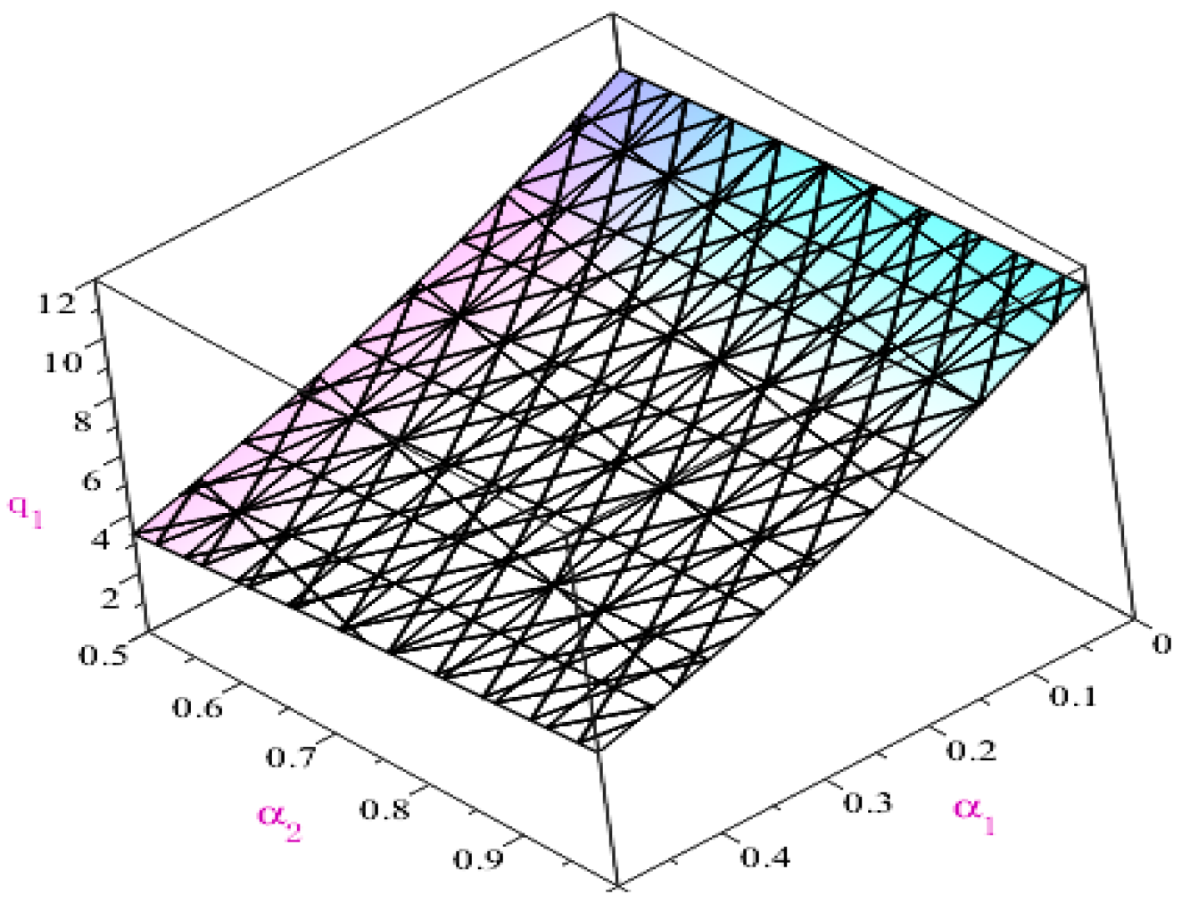
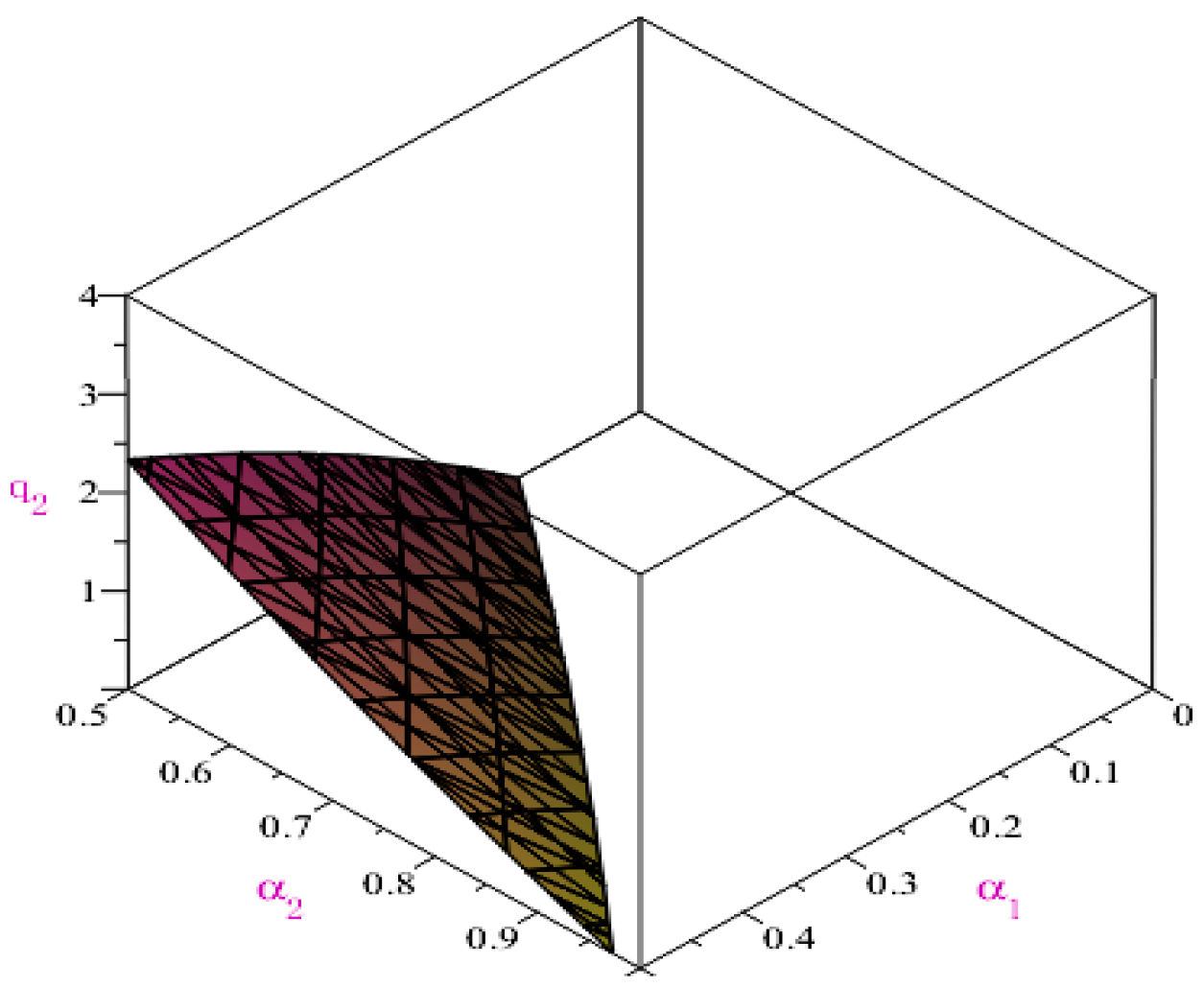
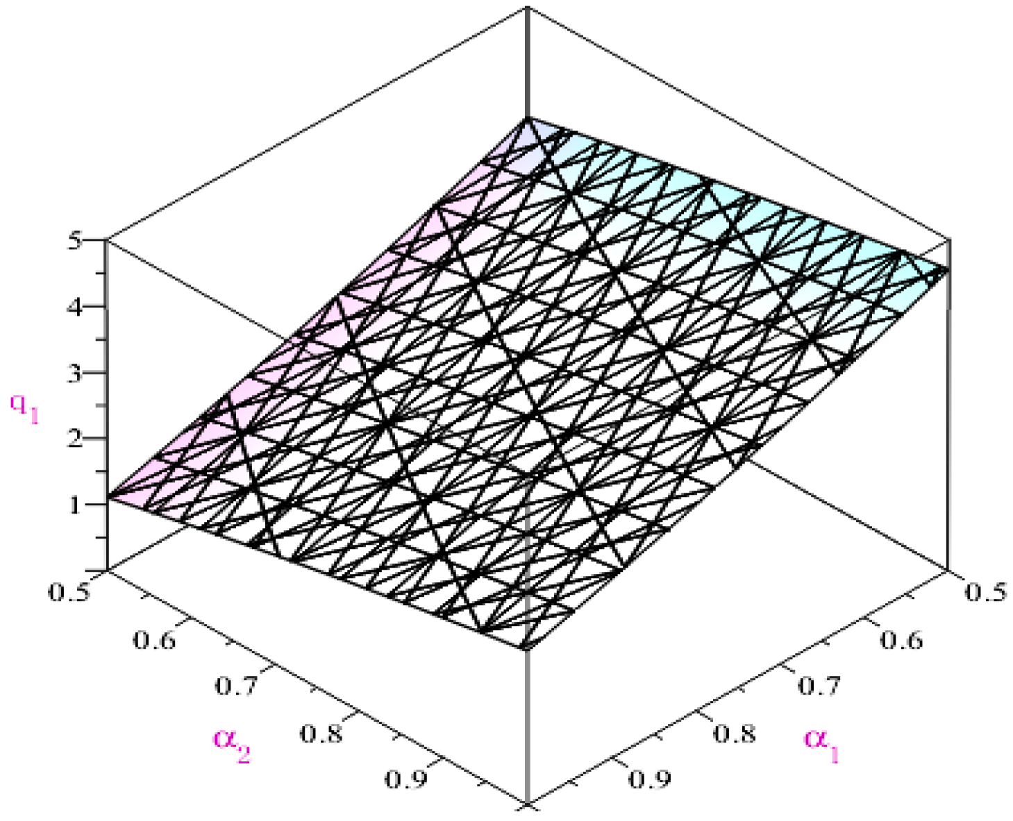
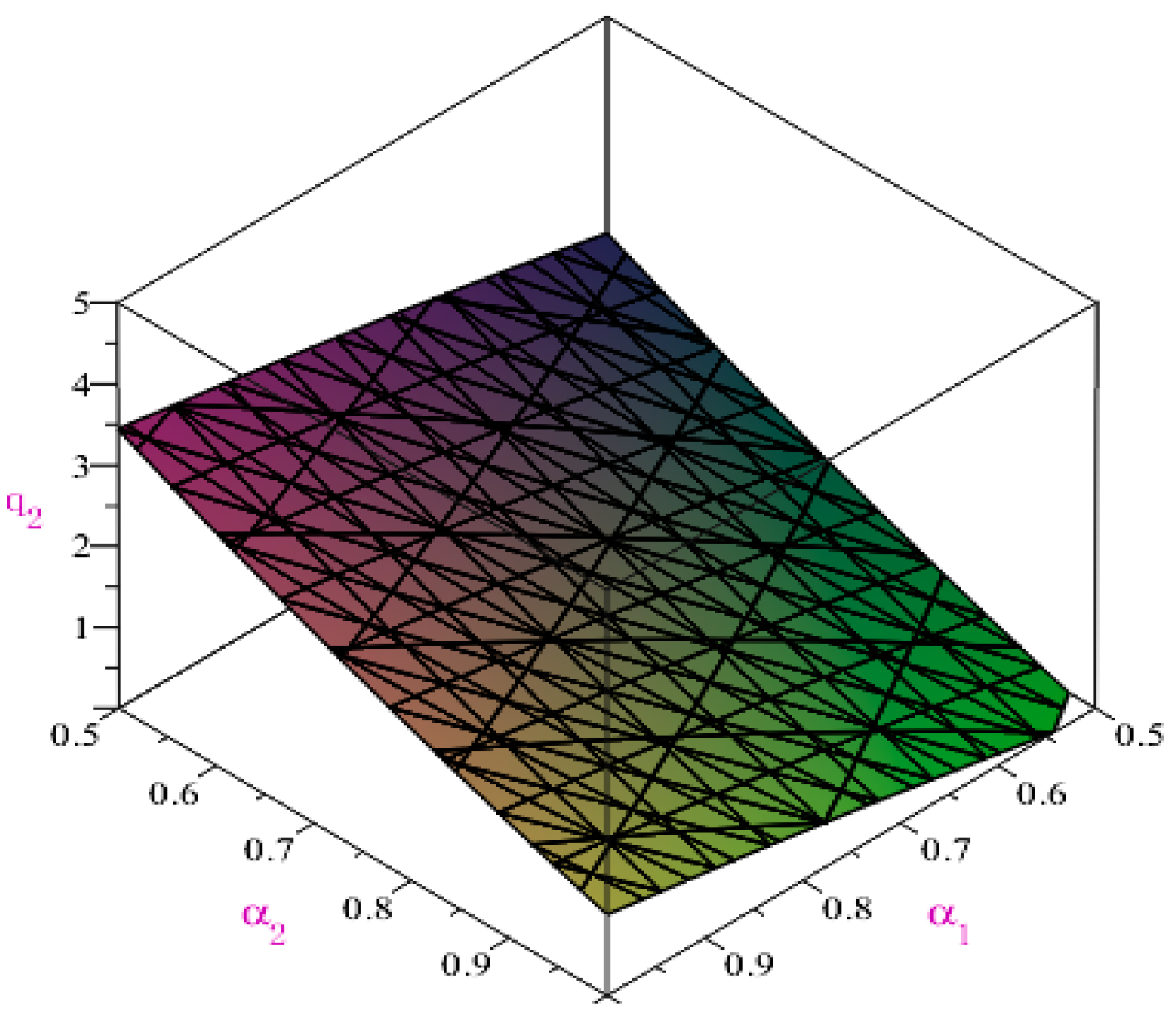
We discuss three scenarios as follows. (1) Given the risk aversion level of CDT, the risk aversion level of AG gradually increases. Let α₁ = 0.3 and α₂ be increasing. (2) Given the risk aversion level of AG, the risk aversion level of CDT gradually increases. Let α₂ = 0.8 and α₁ be increasing. (3) The levels of risk aversion of CDT and AG increase gradually. According to Equations (42), (47) and (48), $q_1^{*},q_2^{*},{\tilde{p}}_1{(q_1^{*},q_2^{*})}_{\sup }({\alpha }_1,{\alpha }_2) \mathrm{and} {\tilde{p}}_2{(q_1^{*},q_2^{*})}_{\sup }({\alpha }_1,{\alpha }_2)$ are shown in

Table 5. (α₁, α₂)-optimistic equilibrium quantity for Scenario II when AG’s risk aversion levels increase.

α1	α2	${\mathit{q}}_{\mathbf{1}}^{*}$	${\mathit{q}}_{\mathbf{2}}^{*}$	${\tilde{\mathit{p}}}_{\mathbf{1}}{({\mathit{q}}_{\mathbf{1}}^{*},{\mathit{q}}_{\mathbf{2}}^{*})}_{\mathbf{s}\mathbf{u}\mathbf{p}}({\mathit{\alpha }}_{\mathbf{1}},{\mathit{\alpha }}_{\mathbf{2}})$	${\tilde{\mathit{p}}}_{\mathbf{2}}{({\mathit{q}}_{\mathbf{1}}^{*},{\mathit{q}}_{\mathbf{2}}^{*})}_{\mathbf{s}\mathbf{u}\mathbf{p}}({\mathit{\alpha }}_{\mathbf{1}},{\mathit{\alpha }}_{\mathbf{2}})$
0.3	0.6	5.7669	0.6935	17.2851	16.3188
0.3	0.7	6.0281	0.1712	17.0553	15.8952
0.3	0.8	6.2706	0	17.1181	15.8230
0.3	0.9	6.4963	0	17.3168	15.9358
0.3	1.0	6.7071	0	17.5022	16.0485

,

Table 6. (α₁, α₂)-optimistic equilibrium quantity for Scenario II when CDT’s risk aversion levels increase.

α1	α2	${\mathit{q}}_{\mathbf{1}}^{*}$	${\mathit{q}}_{\mathbf{2}}^{*}$	${\tilde{\mathit{p}}}_{\mathbf{1}}{({\mathit{q}}_{\mathbf{1}}^{*},{\mathit{q}}_{\mathbf{2}}^{*})}_{\mathbf{s}\mathbf{u}\mathbf{p}}({\mathit{\alpha }}_{\mathbf{1}},{\mathit{\alpha }}_{\mathbf{2}})$	${\tilde{\mathit{p}}}_{\mathbf{2}}{({\mathit{q}}_{\mathbf{1}}^{*},{\mathit{q}}_{\mathbf{2}}^{*})}_{\mathbf{s}\mathbf{u}\mathbf{p}}({\mathit{\alpha }}_{\mathbf{1}},{\mathit{\alpha }}_{\mathbf{2}})$
0.1	0.8	9.1015	0	20.1171	18.9937
0.2	0.8	7.5825	0	18.6176	17.2924
0.3	0.8	6.2706	0	17.1181	15.8230
0.4	0.8	5.1261	0.2584	15.8614	14.8306
0.5	0.8	4.1190	0.7619	14.8810	14.2667

and

Table 7. (α₁, α₂)-optimistic equilibrium quantity for Scenario II when the risk aversion levels for CDT and AG increase.

α1	α2	${\mathit{q}}_{\mathbf{1}}^{*}$	${\mathit{q}}_{\mathbf{2}}^{*}$	${\tilde{\mathit{p}}}_{\mathbf{1}}{({\mathit{q}}_{\mathbf{1}}^{*},{\mathit{q}}_{\mathbf{2}}^{*})}_{\mathbf{s}\mathbf{u}\mathbf{p}}({\mathit{\alpha }}_{\mathbf{1}},{\mathit{\alpha }}_{\mathbf{2}})$	${\tilde{\mathit{p}}}_{\mathbf{2}}{({\mathit{q}}_{\mathbf{1}}^{*},{\mathit{q}}_{\mathbf{2}}^{*})}_{\mathbf{s}\mathbf{u}\mathbf{p}}({\mathit{\alpha }}_{\mathbf{1}},{\mathit{\alpha }}_{\mathbf{2}})$
0.1	0.6	8.5978	0	19.7344	18.5418
0.2	0.7	7.3310	0	18.4188	17.1272
0.3	0.8	6.2706	0	17.1181	15.8230
0.4	0.9	5.3519	0	15.8308	14.6082
0.5	1.0	4.5556	0	14.5022	13.4667

. The variation trend of CDT’s (α₁, α₂)-optimistic equilibrium quantity and the changes of the (α₁, α₂)-optimistic equilibrium quantity of CDT and AG are shown in Figure 3 and Figure 4, respectively.

According to Table 5 and Figure 3 and Figure 4, given α₁ (i.e., CDT’s risk aversion level), the equilibrium quantity of CDT increases gradually with α₂ (i.e., AG’s risk aversion level). For AG, only when α₁ (i.e., CDT’s risk aversion level) and α₂ (i.e., AG’s risk aversion level) meet certain intervals will AG engage in production activities, and its equilibrium quantity is negatively correlated with α₂.

According to Table 6 and Figure 3 and Figure 4, given α₂ (i.e., AG’s risk aversion level), the equilibrium quantity of CDT decreases with α₁ (i.e., CDT’s risk aversion level). For AG, if α₂ (i.e., AG’s risk aversion level) is sufficiently high, AG will not engage in productive activities. Only when α₁ (i.e., CDT’s risk aversion level) and α₂ (i.e., AG’s risk aversion level) meet certain intervals will they engage in production activities, and their equilibrium quantity will be positively correlated with α₁ (i.e., CDT’s risk aversion level).

According to Table 7 and Figure 3 and Figure 4, when α₁ (i.e., CDT’s risk aversion level) and α₂ (i.e., AG’s risk aversion level) increase simultaneously, the equilibrium quantity of CDT gradually decreases. When α₁ (i.e., CDT’s risk aversion level) and α₂ (i.e., AG’s risk aversion level) meet certain intervals and increase simultaneously, AG will engage in production activities and its equilibrium quantity will gradually decrease.

By Equations (47) and (48), if ${\alpha }_1\le 0.5$, $0.5<{\alpha }_2\le 1$, then the market-clearing price of CDT is higher than that of AG. That is, when the risk aversion level of CDT is small and the risk aversion level of AG is large, the market-clearing price of CDT is higher than the market-clearing price of AG.

4.2.3. Scenario III

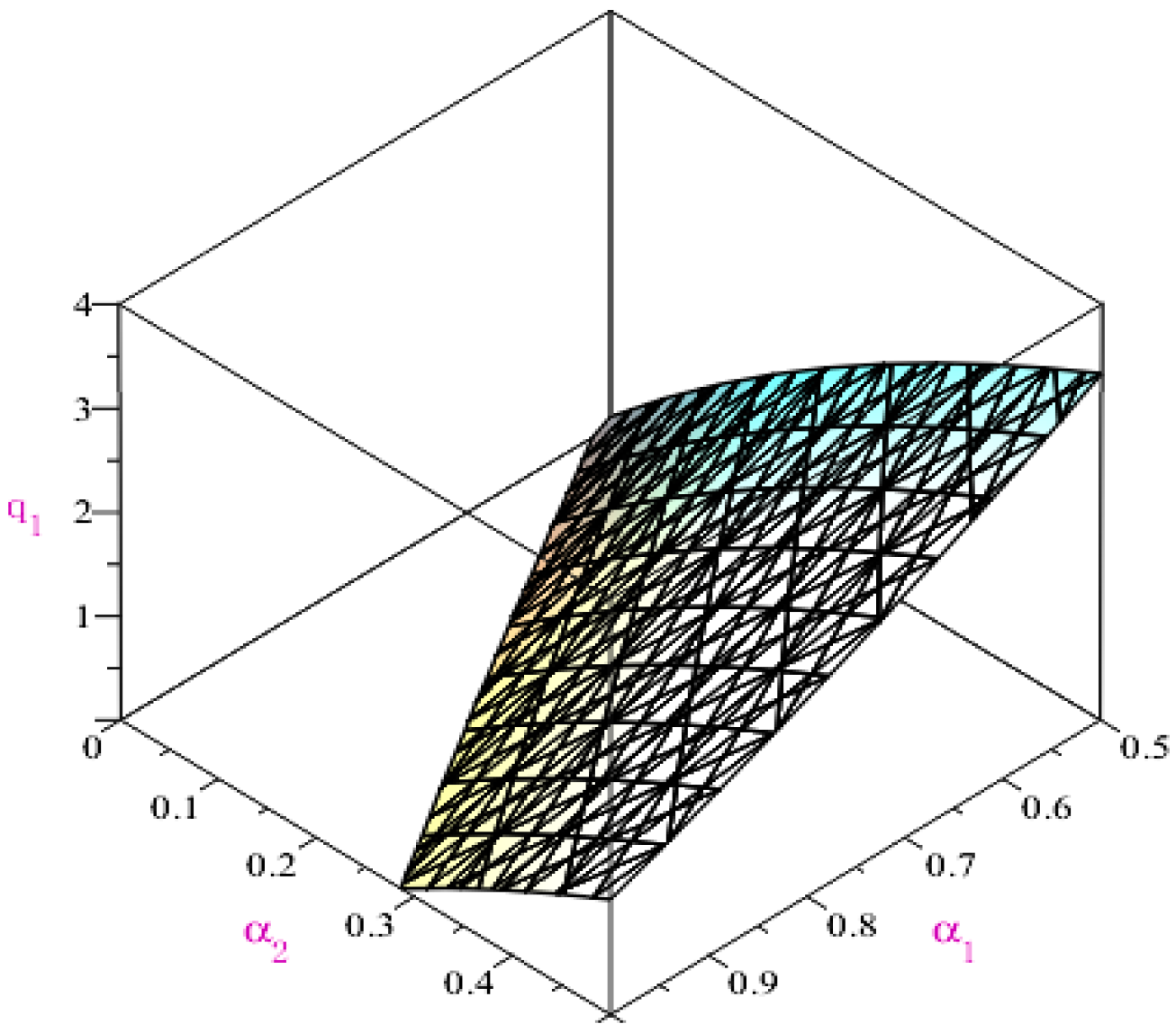
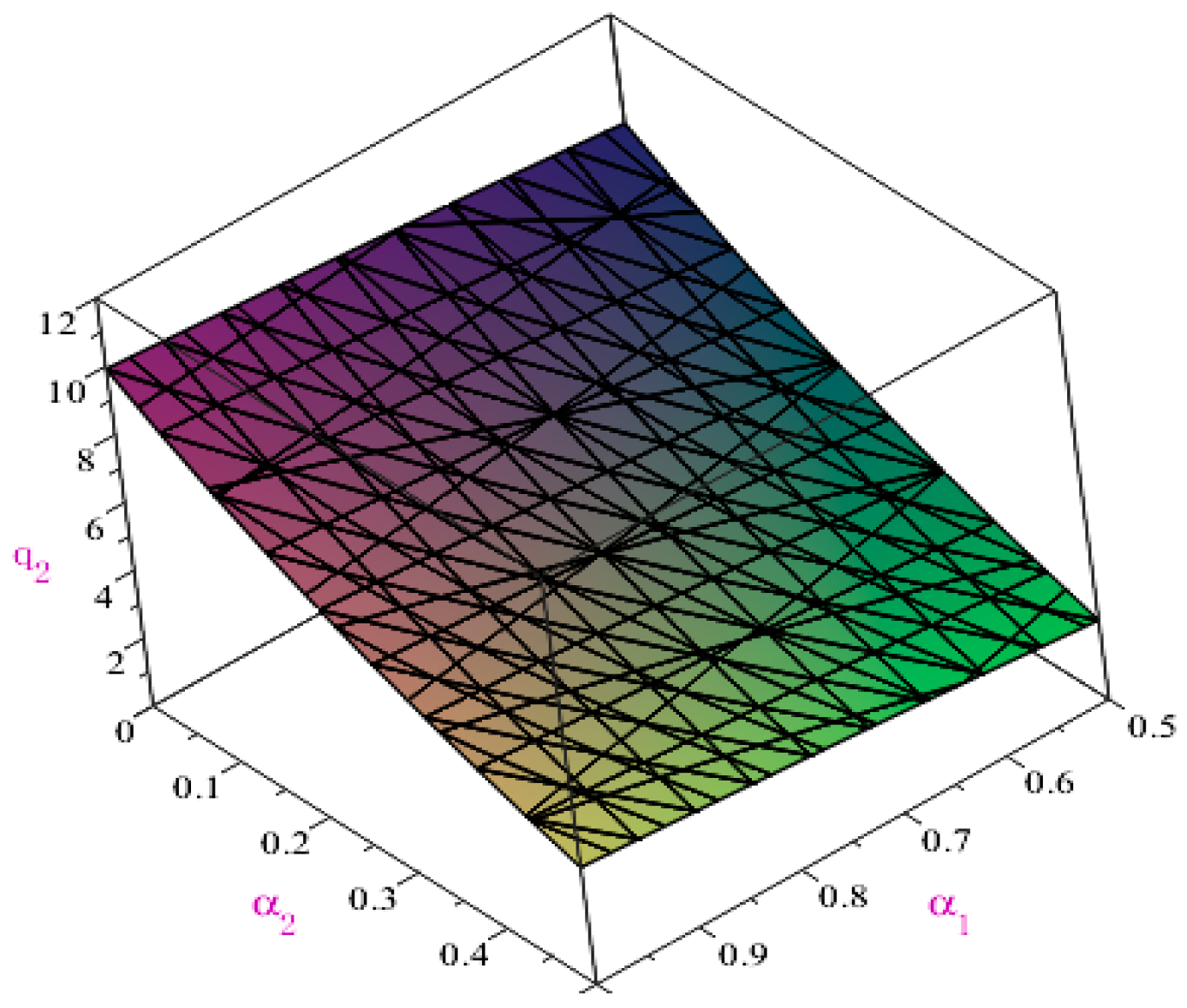
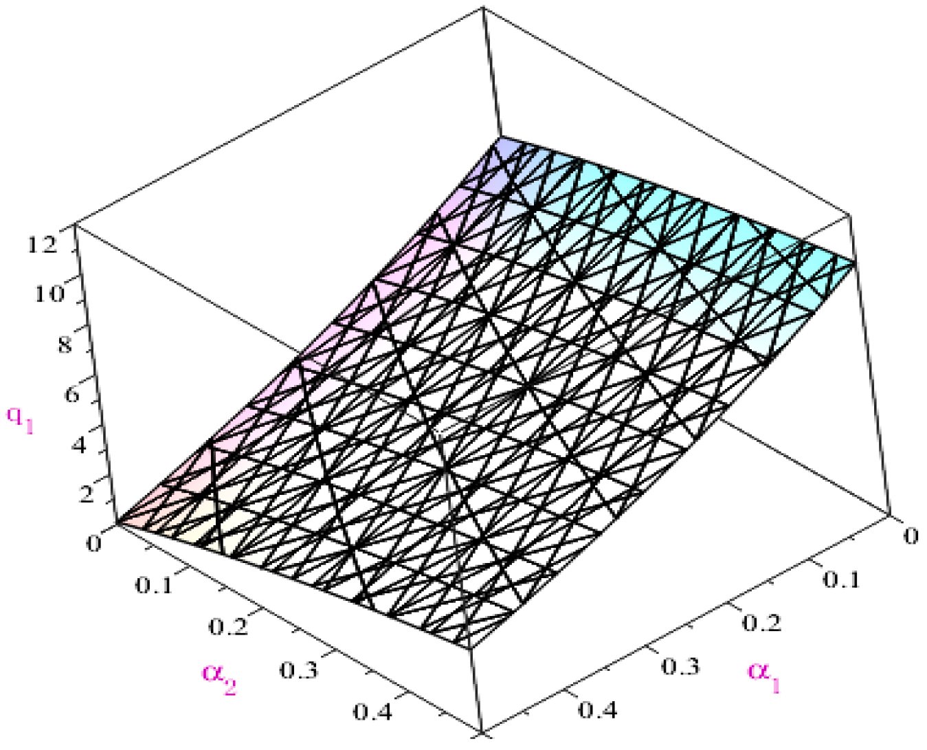
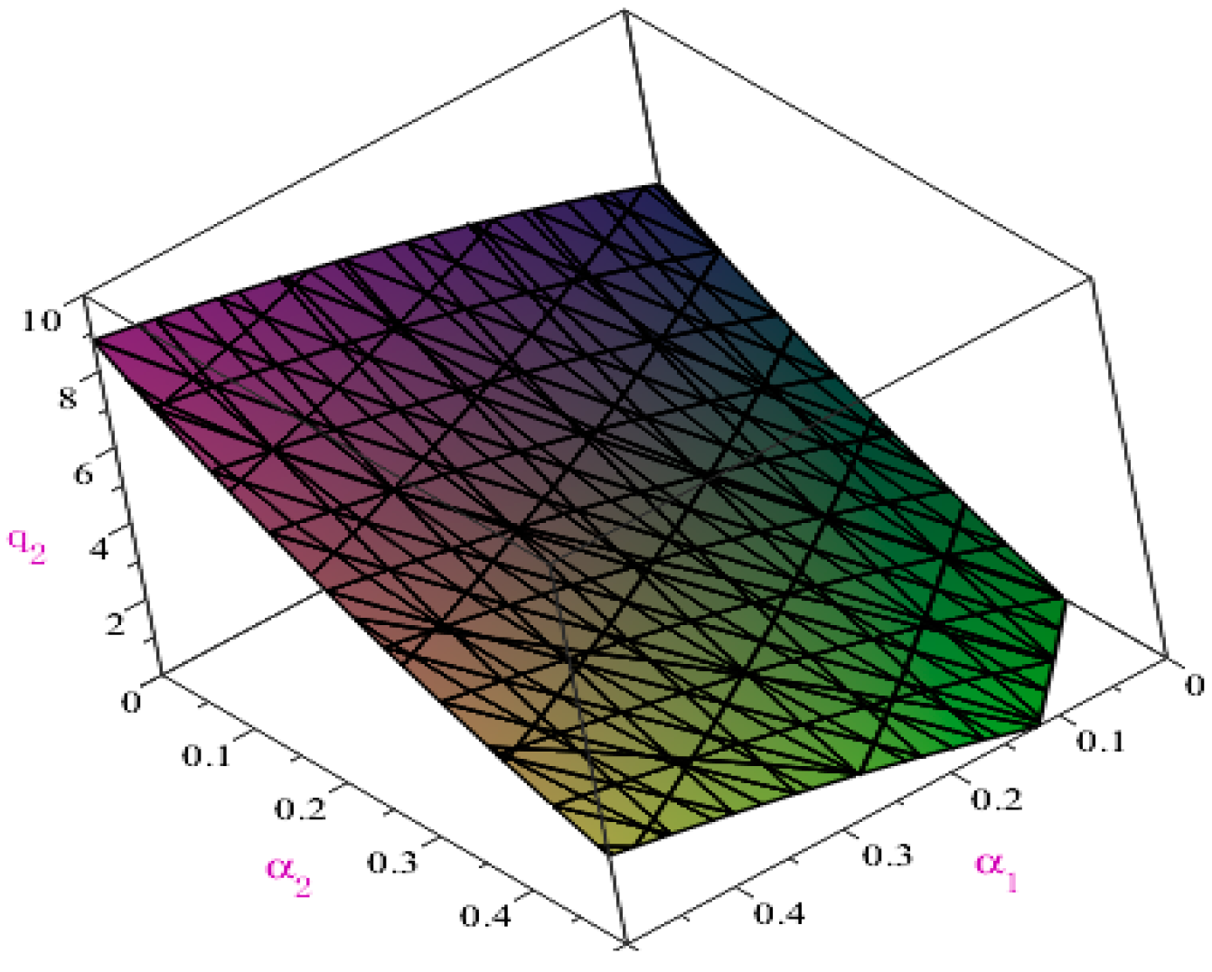
We discuss three scenarios as follows. (1) Given the risk aversion level of CDT, the risk aversion level of AG gradually increases. Let α₁ = 0.8 and α₂ be increasing. (2) Given the risk aversion level of AG, the risk aversion level of CDT gradually increases. Let α₂ = 0.3 and α₁ be increasing. (3) The levels of risk aversion of CDT and AG increase gradually. According to Equations (43), (49) and (50), $q_1^{*}, q_2^{*}, {\tilde{p}}_1{(q_1^{*},q_2^{*})}_{\sup }({\alpha }_1,{\alpha }_2) \mathrm{and} {\tilde{p}}_2{(q_1^{*},q_2^{*})}_{\sup }({\alpha }_1,{\alpha }_2)$ are shown in

Table 8. (α₁, α₂)-optimistic equilibrium quantity for Scenario III when AG’s risk aversion levels increase.

α1	α2	${\mathit{q}}_{\mathbf{1}}^{*}$	${\mathit{q}}_{\mathbf{2}}^{*}$	${\tilde{\mathit{p}}}_{\mathbf{1}}{({\mathit{q}}_{\mathbf{1}}^{*},{\mathit{q}}_{\mathbf{2}}^{*})}_{\mathbf{s}\mathbf{u}\mathbf{p}}({\mathit{\alpha }}_{\mathbf{1}},{\mathit{\alpha }}_{\mathbf{2}})$	${\tilde{\mathit{p}}}_{\mathbf{2}}{({\mathit{q}}_{\mathbf{1}}^{*},{\mathit{q}}_{\mathbf{2}}^{*})}_{\mathbf{s}\mathbf{u}\mathbf{p}}({\mathit{\alpha }}_{\mathbf{1}},{\mathit{\alpha }}_{\mathbf{2}})$
0.8	0.1	0	7.8195	17.5579	19.1429
0.8	0.2	0.2462	6.3647	16.2042	17.8210
0.8	0.3	0.8745	5.1082	15.5006	16.8648
0.8	0.4	1.4225	4.0122	14.8868	15.9086
0.8	0.5	1.9048	3.0476	14.3467	14.9524

,

Table 9. (α₁, α₂)-optimistic equilibrium quantity for Scenario III when CDT’s risk aversion levels increase.

α1	α2	${\mathit{q}}_{\mathbf{1}}^{*}$	${\mathit{q}}_{\mathbf{2}}^{*}$	${\tilde{\mathit{p}}}_{\mathbf{1}}{({\mathit{q}}_{\mathbf{1}}^{*},{\mathit{q}}_{\mathbf{2}}^{*})}_{\mathbf{s}\mathbf{u}\mathbf{p}}({\mathit{\alpha }}_{\mathbf{1}},{\mathit{\alpha }}_{\mathbf{2}})$	${\tilde{\mathit{p}}}_{\mathbf{2}}{({\mathit{q}}_{\mathbf{1}}^{*},{\mathit{q}}_{\mathbf{2}}^{*})}_{\mathbf{s}\mathbf{u}\mathbf{p}}({\mathit{\alpha }}_{\mathbf{1}},{\mathit{\alpha }}_{\mathbf{2}})$
0.6	0.3	1.7902	4.6504	16.2982	17.2677
0.7	0.3	1.3154	4.8878	15.8994	17.0588
0.8	0.3	0.8745	5.1082	15.5006	16.8648
0.9	0.3	0.4640	5.3135	15.1018	16.6841
1.0	0.3	0.0808	5.5052	14.7030	16.5156

and

Table 10. (α₁, α₂)-optimistic equilibrium quantity for Scenario III when the risk aversion levels for CDT and AG increase.

α1	α2	${\mathit{q}}_{\mathbf{1}}^{*}$	${\mathit{q}}_{\mathbf{2}}^{*}$	${\tilde{\mathit{p}}}_{\mathbf{1}}{({\mathit{q}}_{\mathbf{1}}^{*},{\mathit{q}}_{\mathbf{2}}^{*})}_{\mathbf{s}\mathbf{u}\mathbf{p}}({\mathit{\alpha }}_{\mathbf{1}},{\mathit{\alpha }}_{\mathbf{2}})$	${\tilde{\mathit{p}}}_{\mathbf{2}}{({\mathit{q}}_{\mathbf{1}}^{*},{\mathit{q}}_{\mathbf{2}}^{*})}_{\mathbf{s}\mathbf{u}\mathbf{p}}({\mathit{\alpha }}_{\mathbf{1}},{\mathit{\alpha }}_{\mathbf{2}})$
0.6	0.1	0.4345	7.3617	17.7080	19.1251
0.7	0.2	0.6871	6.1442	16.5779	18.0017
0.8	0.3	0.8745	5.1082	15.5006	16.8648
0.9	0.4	1.0120	4.2174	14.4661	15.7156
1.0	0.5	1.1111	3.4444	11.9222	14.5556

. The variation trend of CDT’s (α₁, α₂)-optimistic equilibrium quantity and the changes of the (α₁, α₂)-optimistic equilibrium quantities of CDT and AG are shown in Figure 5 and Figure 6, respectively.

According to Table 8 and Figure 5 and Figure 6, given α₁ (i.e., CDT’s risk aversion level), the equilibrium quantity of AG decreases with α₂ (i.e., AG’s risk aversion level). For CDT, the production of CDT will be carried out only when α₁ (i.e., CDT’s risk aversion level) and α₂ (i.e., AG’s risk aversion level) meet certain intervals, and its equilibrium production is positively correlated with α₂.

According to Table 9 and Figure 5 and Figure 6, given α₂ (i.e., AG’s risk aversion level), the equilibrium quantity of AG increases with α₁ (i.e., CDT’s risk aversion level). For CDT, the production of CDT will be carried out only when α₁ (i.e., CDT’s risk aversion level) and α₂ (i.e., AG’s risk aversion level) meet certain intervals, and its equilibrium production is negatively correlated with α₁.

According to Table 10 and Figure 5 and Figure 6, when α₁ (i.e., CDT’s risk aversion level) and α₂ (i.e., AG’s risk aversion level) increase simultaneously, the equilibrium quantity of AG gradually decreases. When α₁ and α₂ meet certain intervals and increase simultaneously, CDT will engage in production activities and its equilibrium quantity will gradually decrease.

It follows from Equations (49) and (50) that the market-clearing price of CDT is less than that of AG if $0.5<{\alpha }_1\le 1$, ${\alpha }_2\le 0.5$. That is, when the risk aversion level of CDT is high and the risk aversion level of AG is low, the market-clearing price of CDT is less than that of AG.

4.2.4. Scenario IV

We discuss three scenarios as follows. (1) Given the risk aversion level of CDT, the risk aversion level of AG gradually increases. Let α₁ = 0.8 and α₂ be increasing. (2) Given the risk aversion level of AG, the risk aversion level of CDT gradually increases. Let α₂ = 0.8 and α₁ be increasing. (3) The levels of risk aversion of CDT and AG increase gradually. According to Equations (45), (51) and (52), $q_1^{*}, q_2^{*}, {\tilde{p}}_1{(q_1^{*},q_2^{*})}_{\sup }({\alpha }_1,{\alpha }_2) \mathrm{and} {\tilde{p}}_2{(q_1^{*},q_2^{*})}_{\sup }({\alpha }_1,{\alpha }_2)$ are shown in

Table 11. (α₁, α₂)-optimistic equilibrium quantity for Scenario IV when AG’s risk aversion levels increase.

α1	α2	${\mathit{q}}_{\mathbf{1}}^{*}$	${\mathit{q}}_{\mathbf{2}}^{*}$	${\tilde{\mathit{p}}}_{\mathbf{1}}{({\mathit{q}}_{\mathbf{1}}^{*},{\mathit{q}}_{\mathbf{2}}^{*})}_{\mathbf{s}\mathbf{u}\mathbf{p}}({\mathit{\alpha }}_{\mathbf{1}},{\mathit{\alpha }}_{\mathbf{2}})$	${\tilde{\mathit{p}}}_{\mathbf{2}}{({\mathit{q}}_{\mathbf{1}}^{*},{\mathit{q}}_{\mathbf{2}}^{*})}_{\mathbf{s}\mathbf{u}\mathbf{p}}({\mathit{\alpha }}_{\mathbf{1}},{\mathit{\alpha }}_{\mathbf{2}})$
0.8	0.6	2.1868	2.4835	14.0308	14.4571
0.8	0.7	2.4480	1.9612	13.7383	13.9619
0.8	0.8	2.6905	1.4762	13.4667	13.4667
0.8	0.9	2.9163	1.0246	13.2138	12.9714
0.8	1.0	3.1270	0.6032	12.9778	12.4762

,

Table 12. (α₁, α₂)-optimistic equilibrium quantity for Scenario IV when CDT’s risk aversion levels increase.

α1	α2	${\mathit{q}}_{\mathbf{1}}^{*}$	${\mathit{q}}_{\mathbf{2}}^{*}$	${\tilde{\mathit{p}}}_{\mathbf{1}}{({\mathit{q}}_{\mathbf{1}}^{*},{\mathit{q}}_{\mathbf{2}}^{*})}_{\mathbf{s}\mathbf{u}\mathbf{p}}({\mathit{\alpha }}_{\mathbf{1}},{\mathit{\alpha }}_{\mathbf{2}})$	${\tilde{\mathit{p}}}_{\mathbf{2}}{({\mathit{q}}_{\mathbf{1}}^{*},{\mathit{q}}_{\mathbf{2}}^{*})}_{\mathbf{s}\mathbf{u}\mathbf{p}}({\mathit{\alpha }}_{\mathbf{1}},{\mathit{\alpha }}_{\mathbf{2}})$
0.6	0.8	3.6062	1.0183	14.4095	13.9795
0.7	0.8	3.1314	1.2557	13.9381	13.7136
0.8	0.8	2.6905	1.4762	13.4667	13.4667
0.9	0.8	2.2800	1.6814	12.9952	13.2368
1.0	0.8	1.8968	1.8730	12.5238	13.0222

and

Table 13. (α₁, α₂)-optimistic equilibrium quantity for Scenario IV when the risk aversion levels for CDT and AG increase.

α1	α2	${\mathit{q}}_{\mathbf{1}}^{*}$	${\mathit{q}}_{\mathbf{2}}^{*}$	${\tilde{\mathit{p}}}_{\mathbf{1}}{({\mathit{q}}_{\mathbf{1}}^{*},{\mathit{q}}_{\mathbf{2}}^{*})}_{\mathbf{s}\mathbf{u}\mathbf{p}}({\mathit{\alpha }}_{\mathbf{1}},{\mathit{\alpha }}_{\mathbf{2}})$	${\tilde{\mathit{p}}}_{\mathbf{2}}{({\mathit{q}}_{\mathbf{1}}^{*},{\mathit{q}}_{\mathbf{2}}^{*})}_{\mathbf{s}\mathbf{u}\mathbf{p}}({\mathit{\alpha }}_{\mathbf{1}},{\mathit{\alpha }}_{\mathbf{2}})$
0.6	0.6	3.1026	2.0256	14.9333	14.9333
0.7	0.7	2.8889	1.7407	14.2000	14.2000
0.8	0.8	2.6905	1.4762	13.4667	13.4667
0.9	0.9	2.5057	1.2299	12.7333	12.7333
1.0	1.0	2.3333	1.0000	12.0000	12.0000

. The variation trend of CDT’s (α₁, α₂)-optimistic equilibrium quantity and the changes of the (α₁, α₂)-optimistic equilibrium quantities of CDT and AG are shown in Figure 7 and Figure 8, respectively.

According to Table 11 and Figure 7 and Figure 8, given α₁ (i.e., CDT’s risk aversion level), the equilibrium quantity of CDT increases gradually with α₂ (i.e., AG’s risk aversion level), while the equilibrium quantity of AG will gradually decrease. According to Table 13 and Figure 7 and Figure 8, if α₁ and α₂ are increasing simultaneously, the equilibrium quantity of CDT and AG will decrease. In addition, it follows from Equations (51) and (52) that the market-clearing price for CDT and AG will be equal if they have the same confidence level (i.e., risk aversion level).

5. Conclusions

The extant research on the Cournot game model is mainly based on the assumption that the decision maker is completely rational. However, the decisions of the decision maker are more or less influenced by his own behavioral characteristics and psychological preferences in many real situations. In the fuzzy environment, this paper studies the Cournot game between two manufacturers with risk aversion. Based on credibility theory, this paper describes the risk aversion behavior of manufacturers by using the optimistic value criterion and constructs the fuzzy Cournot game model with risk aversion. The definition of optimistic equilibrium quantity and its existence theorem are shown. Finally, a case is used to illustrate the effectiveness and significance of the model proposed in this paper. The sensitivity of optimistic equilibrium quantity with respect to confidence level (or risk aversion levels) is analyzed, and the effect of manufacturers’ risk aversion levels on the market-clearing price is discussed. It is shown that manufacturers’ optimistic equilibrium quantity is positively related to the risk aversion levels of their competitors and negatively related to their own risk aversion levels if the two manufacturers show risk aversion preferences. It is also shown that the market-clearing price of a manufacturer with a higher risk aversion level is less than that of another with a lower risk aversion level.

In this paper, the Cournot game with risk aversion is considered under the fuzzy environment. The conclusions have stronger explanatory ability for the actual situation. However, the model constructed in this paper fails to address the case where two manufacturers show loss aversion, fairness concerns, reciprocal altruistic behavior, and so on. Therefore, the Cournot game with other behavior of bounded rationality will be an interesting exploration. In addition, our work focuses on the equilibrium quantity when the parameters in the credibilistic Cournot game are denoted by the triangular fuzzy numbers. However, it is still unknown whether the equilibrium quantity exists when the parameters in the credibilistic Cournot game are denoted by other fuzzy numbers, such as the interval fuzzy numbers, the trapezoidal fuzzy numbers, etc. Therefore, future research will focus on exploring the existence of the equilibrium quantity when the parameters of the credibilistic Cournot game are other fuzzy numbers.

References

1. Zadeh, L.A. Fuzzy sets. Inf. Control 1965, 8, 338–353. [Google Scholar] [CrossRef] [Green Version]
2. Yao, J.-S.; Wu, K. Consumer surplus and producer surplus for fuzzy demand and fuzzy supply. Fuzzy Sets Syst. 1999, 103, 421–426. [Google Scholar] [CrossRef]
3. Wu, K.; Yao, J.-S. Fuzzy inventory with backorder for fuzzy order quantity and fuzzy shortage quantity. Eur. J. Oper. Res. 2003, 150, 320–352. [Google Scholar] [CrossRef]
4. Ouyang, L.-Y.; Yao, J.-S. A minimax distribution free procedure for mixed inventory model involving variable lead time with fuzzy demand. Comput. Oper. Res. 2002, 29, 471–487. [Google Scholar] [CrossRef]
5. Yao, J.-S.; Wu, K. The best prices of two mutual complements in the fuzzy sense. Fuzzy Sets Syst. 2000, 111, 433–454. [Google Scholar] [CrossRef]
6. Yao, J.-S.; Chang, S.-C. Economic principle on profit in the fuzzy sense. Fuzzy Sets Syst. 2001, 117, 113–127. [Google Scholar] [CrossRef]
7. Yao, J.-S.; Shih, T.-S. Fuzzy revenue for fuzzy demand quantity based on interval-valued fuzzy sets. Comput. Oper. Res. 2002, 29, 1495–1535. [Google Scholar] [CrossRef]
8. Xu, R.; Zhai, X. Optimal models for single-period supply chain problems with fuzzy demand. Inf. Sci. 2008, 178, 3374–3381. [Google Scholar] [CrossRef]
9. Liang, G.S.; Lin, L.Y.; Liu, C.F. The optimum output quantity of a duopoly market under a fuzzy decision environment. Comput. Math. Appl. 2008, 56, 1176–1187. [Google Scholar] [CrossRef] [Green Version]
10. Wang, C.; Tang, W.; Zhao, R. Static Bayesian games with finite fuzzy types and the existence of equilibrium. Inf. Sci. 2008, 178, 4688–4698. [Google Scholar] [CrossRef]
11. Dang, J.-F.; Hong, I.-H. The Cournot game under a fuzzy decision environment. Comput. Math. Appl. 2010, 59, 3099–3109. [Google Scholar] [CrossRef] [Green Version]
12. Dang, J.-F.; Hong, I.-H.; Lin, J.-M. The Cournot production game with multiple firms under an ambiguous decision environment. Inf. Sci. 2014, 266, 186–198. [Google Scholar] [CrossRef]
13. Tan, C.; Liu, Z.; Wu, D.D.; Chen, X. Cournot game with incomplete information based on rank-dependent utility theory under a fuzzy environment. Int. J. Prod. Res. 2016, 56, 1789–1805. [Google Scholar] [CrossRef]
14. Driesen, B.; Perea, A.; Peters, H. Alternating offers bargaining with loss aversion. Math. Soc. Sci. 2012, 64, 103–118. [Google Scholar] [CrossRef] [Green Version]
15. Feng, Z.; Tan, C. Subgame Perfect Equilibrium in the Rubinstein Bargaining Game with Loss Aversion. Complexity 2019, 2019, 5108652. [Google Scholar] [CrossRef] [Green Version]
16. Gimpel, H. Loss Aversion and Reference-Dependent Preferences in Multi-Attribute Negotiations. Group Decis. Negot. 2007, 16, 303–319. [Google Scholar] [CrossRef]
17. Shalev, J. Loss Aversion and Bargaining. Theory Decis. 2002, 52, 201–232. [Google Scholar] [CrossRef]
18. Roth, A.E. Game-Theoretic Models of Bargaining; Cambridge University Press: Cambridge, UK, 1985. [Google Scholar]
19. Volij, O.; Winter, E. On risk aversion and bargaining outcomes. Games Econ. Behav. 2002, 41, 120–140. [Google Scholar] [CrossRef] [Green Version]
20. Feng, Z.; Tan, C.; Zhang, J.; Zeng, Q. Bargaining Game with Altruistic and Spiteful Preferences. Group Decis. Negot. 2021, 30, 277–300. [Google Scholar] [CrossRef]
21. Montero, M. Altruism, Spite and Competition in Bargaining Games. Theory Decis. 2008, 65, 125–151. [Google Scholar] [CrossRef]
22. Hyndman, K. Repeated bargaining with reference-dependent preferences. Int. J. Game Theory 2011, 40, 527–549. [Google Scholar] [CrossRef]
23. Kawamori, T. Bilateral bargaining with endogenous status quo. Econ. Lett. 2019, 185, 108699. [Google Scholar] [CrossRef]
24. Li, D. Bargaining with history-dependent preferences. J. Econ. Theory 2007, 136, 695–708. [Google Scholar] [CrossRef] [Green Version]
25. Goeree, J.K.; Holt, C.A.; Palfrey, T.R. Risk averse behavior in generalized matching pennies games. Games Econ. Behav. 2003, 45, 97–113. [Google Scholar] [CrossRef] [Green Version]
26. Sabater-Grande, G.; Georgantzis, N. Accounting for risk aversion in repeated prisoners’ dilemma games: An experimental test. J. Econ. Behav. Organ. 2002, 48, 37–50. [Google Scholar] [CrossRef]
27. Engelmann, D.; Steiner, J. The effects of risk preferences in mixed-strategy equilibria of games. Games Econ. Behav. 2007, 60, 381–388. [Google Scholar] [CrossRef] [Green Version]
28. Gao, J.; Yang, X. Credibilistic Bimatrix Game with Asymmetric Information: Bayesian Optimistic Equilibrium Strategy. Int. J. Uncertain. Fuzziness Knowl. Based Syst. 2013, 21, 89–100. [Google Scholar] [CrossRef]
29. Tan, C.; Feng, Z.; Li, C.; Yi, W. Optimal Bayesian equilibrium for n-person credibilistic non-cooperative game with risk aversion. J. Intell. Fuzzy Syst. 2017, 33, 741–751. [Google Scholar] [CrossRef]
30. Gao, J.; Liu, Z.-Q.; Shen, P. On characterization of credibilistic equilibria of fuzzy-payoff two-player zero-sum game. Soft Comput. 2009, 13, 127–132. [Google Scholar] [CrossRef]
31. Feng, Z.; Tan, C. Credibilistic Bimatrix Games with Loss Aversion and Triangular Fuzzy Payoffs. Int. J. Fuzzy Syst. 2020, 22, 1635–1652. [Google Scholar] [CrossRef]
32. Liu, B.; Liu, Y.-K. Expected value of fuzzy variable and fuzzy expected value models. IEEE Trans. Fuzzy Syst. 2002, 10, 445–450. [Google Scholar] [CrossRef]
33. Liu, B. Uncertainty Theory; Springer: Berlin/Heidelberg, Germany, 2007. [Google Scholar]
34. Gao, J.; Liu, B. New primitive chance measures of fuzzy random event. Int. J. Fuzzy Syst. 2001, 3, 527–531. [Google Scholar]
35. Dubois, D.; Prade, H. Fuzzy Sets and Systems: Theory and Applications; Academic Press: New York, NY, USA, 1980. [Google Scholar]
36. Wu, Q. Fuzzy robust ν-support vector machine with penalizing hybrid noises on symmetric triangular fuzzy number space. Expert Syst. Appl. 2011, 38, 39–46. [Google Scholar] [CrossRef]
37. He, Y.; Zhou, D.; Wang, Q. Study on priority method for triangular fuzzy number complementary judgment matrix based on possibility degree. Oper. Res. Manag. Sci. 2009, 18, 65–68. [Google Scholar]
38. Chen, X.; Huang, Z.L.; Luo, J. Approach for triangular fuzzy number-based uncertain multi-attribute decision making based on relative similarity degree relation. Control Decis. 2016, 31, 2232–2240. [Google Scholar]
Figure 1. Changes of q 1 * with α1 and α2 ( α 1 0.5 , α 2 0.5 ).
Mathematics 11 01029 g001
Figure 2. Changes of q 2 * with α1 and α2 ( α 1 0.5 ,   α 2 0.5 ).
Mathematics 11 01029 g002
Figure 3. Changes of q 1 * with α1 and α2 ( α 1 0.5 ,   0.5 < α 2 1 ).
Mathematics 11 01029 g003
Figure 4. Changes of q 2 * with α1 and α2 ( α 1 0.5 ,   0.5 < α 2 1 ).
Mathematics 11 01029 g004
Figure 5. Changes of q 1 * with α1 and α2 ( 0.5 < α 1 1 ,   α 2 0.5 ).
Mathematics 11 01029 g005
Figure 6. Changes of q 2 * with α1 and α2 ( 0.5 < α 1 1 ,   α 2 0.5 ).
Mathematics 11 01029 g006
Figure 7. Change of q 1 * with α1 and α2 ( 0.5 < α 1 1.0 ,   0.5 < α 2 1.0 ).
Mathematics 11 01029 g007
Figure 8. Change of q 2 * with α1 and α2 ( 0.5 < α 1 1.0 ,   0.5 < α 2 1.0 ).
Mathematics 11 01029 g008