Numerical Simulation of Heat Transfer and Spread of Virus Particles in the Car Interior

Abstract

The epidemic caused by the coronavirus infection SARS-CoV-2 at the beginning of 2022 affected approximately 500 million people in all countries. The source of infection is the particles of the virus, which, when breathing, talking, and coughing, are released with the respiratory droplets and aerosol dust of an infected person. Actions aimed at combating and minimizing the consequences of coronavirus infection led to taking measures in scientific areas to investigate the processes of the spread of viral particles in the air, in ventilation, and air conditioning systems of premises and transport, filtration through masks, the effect of partitions, face shields, etc. The article presents a mathematical model of the spread of viral particles in technological transport. Air intake diverters and the operator’s respiratory tract are the sources of the virus. The Euler–Lagrange approach was used to simulate liquid droplets in a flow. Here, the liquid phase is considered as a continuous medium using Navier–Stokes equations, the continuity equation, the energy equation, and the diffusion equation. Accounting for diffusion makes it possible to explicitly model air humidity and is necessary to consider the evaporation of droplets (changes in the mass and size of particles containing the virus). Liquid droplets are modeled using the discrete-phase model (DPM), in which each particle is tracked in a Lagrange coordinate system. The DPM method is effective, since the volume fraction of particles is small relative to the total volume of the medium, and the interaction of particles with each other can be neglected. In this case, the discrete and continuous phases are interconnected through the source terms in the equations. The averaged RANS equations are solved numerically using the k-ω turbulence model in the Ansys Fluent package. The task was solved in a static form and in the time domain. For a non-stationary problem, the stabilization time of the variables is found. The simulation results are obtained in the form of fields of pressures, velocities, temperatures and air densities, and the field of propagation of particles containing the virus. Various regimes were studied at various free flow rates and initial velocities of droplets with viral particles. The results of trajectories and velocities of particles, and particle concentrations depending on time, size, and on the evaporability of particles are obtained.

1. Introduction

One of the urgent tasks of thermal comfort and maintaining safe vehicle operating conditions (HVAC) is the task of maintaining comfortable temperatures, speed, and air humidity in the area of the machine operator (Figure 1). Creating a microclimate in the cab is the most essential goal of ensuring optimal conditions for human HVAC operation.

The factors that provide a comfortable microclimate and the theoretical foundations for modeling the microclimate in cabins based on the balance equations of heat flows are presented in [1,2,3,4,5], “the processes of convective heat exchange with the environment are described” [6,7,8,9,10].

Many analytical works relate to the actual problem of finding the heat transfer coefficients from the Nusselt criterion for harvesting machines [11], SUV vehicles [12,13,14,15,16], building elements [17], machinery cabins [18,19,20,21,22], and engineering systems [23,24,25]. This approach allows only internal regions to be considered, and thermal boundary conditions are modeled using heat transfer coefficients. This method makes it possible to obtain sufficiently accurate solutions only in the absence of large flow gradients along the walls inside and outside the domain.

The methods of computational fluid dynamics make it possible to obtain the solution of hydrodynamic equations in numerical form, taking into account complex boundary conditions. Thus, in [26,27,28,29,30,31] the results of numerical studies and the values of heat transfer coefficients for various tubular heat exchangers, in evaporators, coolers, and other surfaces are presented. In papers [32,33,34,35,36], different models of turbulence are considered depending on the viscosity and flow parameters, as well as the roughness of the domain walls. New numerical approaches for flow and engineering problems are discussed in [37,38]. The papers [39,40,41,42,43,44,45] present the results of a CFD analysis of thermal and hydrodynamic characteristics in various vehicles and consider optimization issues for various cab configurations and geometries. The results of these works were obtained based on the numerical solution mainly by the RANS Navier–Stokes equations, without taking into account air humidity and the particle motion model.

The epidemic caused by the coronavirus infection SARS-CoV-2 at the beginning of 2022 affected approximately 500 million people in all countries. The source of infection is the particles of the virus, which, when breathing, talking, and coughing, are released with the respiratory droplets and aerosol dust of an infected person. Measures aimed at combating and minimizing the consequences of coronavirus infection led to the need for a number of scientific studies to study the processes of the spread of viral particles in the air, in ventilation, and in air conditioning systems of premises and transport, as well as the filtration through masks, and the effect of partitions and face shields, etc.

The CFD approach to the study of the spread of viral particles was used to simulate the transmission of the virus in urban public places [46,47], considering different landscape designs and air speeds, in rooms with different partitions [48,49,50,51,52], risks assessment [53,54,55], and construction drainage pipes [56]. Options for optimizing ventilation and air conditioning systems are considered, including the spread of a part of the virus in buildings [57], buses and trains [58,59], and in two-phase flow systems [60,61,62,63]. The studies under consideration present models of particle motion in relatively large spaces. The results were obtained numerically by solving the averaged Navier–Stokes equations in software packages. The focus is on human-to-human transmission of viruses. However, the presented works did not simulate the movement of particles in technological transport, which are usually single-seated, and the main attention should be paid to the effective removal of viruses from the cabin.

This study is part of a larger effort to develop a new type of cab for special vehicles with improved energy efficiency and driver safety. These cabins, as a rule, are single-seated, and are used for agricultural, road, and other special equipment. Previously, in [22], a method was developed for obtaining heat transfer coefficients through a multilayer wall and cabin windows, and comparisons were made with applied theories.

The purpose of this article is to develop a numerical method for calculating the spread of pathogen particles considering the volatility of droplets, based on Navier–Stokes equations using the turbulence approach, energy and diffusion models, and a discrete-phase formula for modeling particles. The internal and domain of cabin air are considered and heat exchange with the environment is carried out through heat transfer coefficients. Ansys Fluent was used as a software for numerical analysis of the computer fluid dynamics. This method allows us to obtain fields of all air characteristics, trajectories, and particle sizes, considering their evaporation at any time.

The problem was solved in a static formulation and in the time domain. The fields of pressures, velocities, air distribution densities, and the distribution fields of particles containing coronavirus were calculated. Various rates and sources of entry of pathogen particles were studied.

The significance of this work lies in the following:

In the field of theoretical research, the resulting numerical model makes it possible to determine the trajectories, velocities, and temperature and humidity characteristics of air flows and particles in the air (viruses), which reduces the time for creating air conditioning devices in machines.

In the practical field, results have been obtained that allow manufacturers to design improved air conditioning devices to create a comfortable and safe environment for the operator.

2. Materials and Methods

2.1. Problem Statement of Simulation Liquid Droplets in a Flow

The assumption of the Euler–Lagrange approach is to simulate liquid droplets in a flow. The liquid phase is considered as a continuous continuum using the Navier–Stokes Equation (1) together with the continuity Equation (2) [3,4].

$$\frac{\partial \mathit{u}}{\partial t}+\left(\mathit{u}·\nabla \right)\mathit{u}=\mathit{X}-\frac{1}{\rho }\nabla p+\eta \Delta \mathit{u}+\frac{1}{3}\eta \nabla \nabla ·\mathit{u},$$

(1)

$$\frac{\partial \rho }{\partial t}+\nabla ·\left(\rho \mathit{u}\right)=0,$$

(2)

Here $\mathit{u}=\mathit{u}\left(x,y,z,t\right)$ is medium velocity in Euler variables; $p=p\left(x,y,z,t\right)$ is pressure; $\rho =\rho \left(x,y,z,t\right)$ is density; $\eta =\frac{\mu }{\rho }, \mu \mathrm{and}\eta$ dynamic and kinematic viscosities, respectively, μ is assumed to be constant; and $\mathit{X}=\mathit{X}\left(x,y,z,t\right)$ − body forces.

To consider the mass amount of water vapor in the air, energy Equation (3) is used to take into account temperature, considering diffusion and mass transfer Equations (4) and (5) [6,7,8,9,10]:

$$\frac{\partial T}{\partial t}+\mathit{u}\nabla T=\frac{\lambda }{{\mathrm{c}}_{\rho }\rho }\Delta T-\nabla ·{\displaystyle \sum }_{i=1}^n{\mathit{J}}_i+\varphi ,$$

(3)

$$\frac{\partial \rho Y_i}{\partial t}+\nabla ·\left(\rho \mathit{u}{Y}_i\right)=\nabla ·{\mathit{J}}_i+S_i, i=1\dots N-1,$$

(4)

$${\displaystyle \sum }_{i=1}^n{Y}_i=1.$$

(5)

Here, $T=T\left(x,y,z,t\right)$ is temperature; λ and ${\mathrm{c}}_{\rho }$ are thermal conductivity and specific heat capacity, they are considered constant; ϕ and S_i are internal sources of heat and diffusion; Y_i is local mass fraction of i substance; and ${\mathit{J}}_i$ is diffuse flow of the i substance, which occurs due to the gradient of concentrations, temperature, and pressure, and the turbulent case is written as follows:

$${\mathit{J}}_i=\left(\mathsf{\rho }{D}_{i,m}+\frac{{\mu }_t}{S{c}_t}\right)\nabla Y_i+D_{i,T}\frac{\nabla T}{T}+D_{i,p}\frac{\nabla p}{p}.$$

(6)

Here, $S{c}_t$ is the turbulent Schmidt number; ${\mu }_t$ is the turbulent viscosity; $D_{i,m}$ are the mass diffusion coefficients; $D_{i,T}$ are the thermal diffusion coefficients (thermal diffusion coefficients); and $D_{i,p}$ are the barotropic diffusions of the i-th substance. The last barotropic term in (6) is considered in the presence of a large pressure gradient.

Diffusion coefficients characterize the diffusion rate, which is equal to the amount of a substance passing per unit of time through a section of a unit area, caused by a gradient of concentration, temperature, and pressure, respectively.

The Mendeleev–Clapeyron relation (7) is used as the ideal gas law [3].

$$p=\frac{\rho TR}{M},$$

(7)

where R and M are the gas constant and the molar mass, respectively.

2.2. Particles Motion Simulation by the Discrete Phase Model (DPM)

To simulate liquid drops, the discrete phase model (DPM) [29,56] was applied, in which every particle was tracked in a Lagrangian frame of reference.

The DPM method is efficient enough at a volume fraction of particles of no more than 0.1 of the liquid, so that the interaction of particles with each other can be neglected. In this assumption, the discrete and continuous phases are interconnected through source terms in the equations.

The main assumption of the particle motion model is described by the following equations:

The balance of power equation:

$$\frac{m_{p}d{\mathit{u}}_p}{dt}={\mathit{F}}_p^d+{\mathit{F}}_p^o,$$

(8)

Here, $m_p$ is the mass of the particle; ${\mathit{u}}_p$ is the velocity vector of the particle; ${\mathit{F}}_p^o$ are additional forces, in particular, gravitational force, lifting force, etc.; and ${\mathit{F}}_p^d$ is the force of the particle resistance of interaction with the liquid phase.

The balance of power equation:

$${\mathit{F}}_p^d=m_p\frac{\mathit{u}-{\mathit{u}}_p}{{\tau }_r},$$

(9)

$${\tau }_r=\frac{{\rho }_p{d}_p^2}{18\mu }\frac{24}{C_{d}Re},$$

(10)

$$Re=\frac{\rho d_p\left|{\mathit{u}}_p-\mathit{u}\right|}{\mu },$$

(11)

Here, µ is the fluid dynamic viscosity; d_p is the particle diameter; Re is the Reynolds number; and C_d is aerodynamic drag coefficient, and in the case of spherical drops can be represented as:

$$C_d=a_1+\frac{a_2}{Re}+\frac{a_3}{R{e}^2},$$

(12)

Here a_i are constants [60].

To simulate the rotation of a particle, the momentum balance equation is used:

$$I_p\frac{d{\mathit{\omega }}_p}{dt}=\frac{\rho }{2}{\left(\frac{d_p}{2}\right)}^5{C}_{\omega }\left|\Omega \right|\Omega ,$$

(13)

$$\Omega =\frac{1}{2}\nabla \times \mathit{u}-{\mathit{\omega }}_p,$$

(14)

where I_p is a moment of inertia of the particle; ${\mathit{\omega }}_p$ is a vector of the angular velocity of the particle; Ω is the relative angular velocity; and $C_{\omega }$ is the coefficient of aerodynamic resistance to rotation [58]:

$$C_{\omega }=\frac{6.45}{\sqrt{R{e}_{\omega }}}+\frac{32.1}{R{e}_{\omega }},$$

(15)

$$R{e}_{\omega }=\frac{\rho \Omega d_p^2}{4\mu }.$$

(16)

To consider the evaporation of a drop, the following equation is used [58]:

$$\frac{d{m}_p}{dt}=h_p{A}_p\rho \ln \left(1+B_m\right),$$

(17)

Here, h_p is the heat transfer coefficient; A_p is the surface area of the particle; and B_p is determined by the formula:

$$B_p=\frac{Y_i^s-Y_i^{out}}{1-Y_i^s},$$

(18)

Here, $Y_i^s$ is the mass fraction of vapor on the particle surface and $Y_i^{out}$ is the mass fraction of vapor in the continuum.

The energy equation for modeling heat transfer between a drop and a medium is written in the following form:

$$m_p{c}_p^p\frac{d{T}_p}{dt}=h_p\left(T_{out}-T_p\right),$$

(19)

Here, $c_p^p$ is the heat capacity of the particle; T_out is the temperature of the medium; and T_p is the temperature of the particle.

2.3. Boundary Conditions

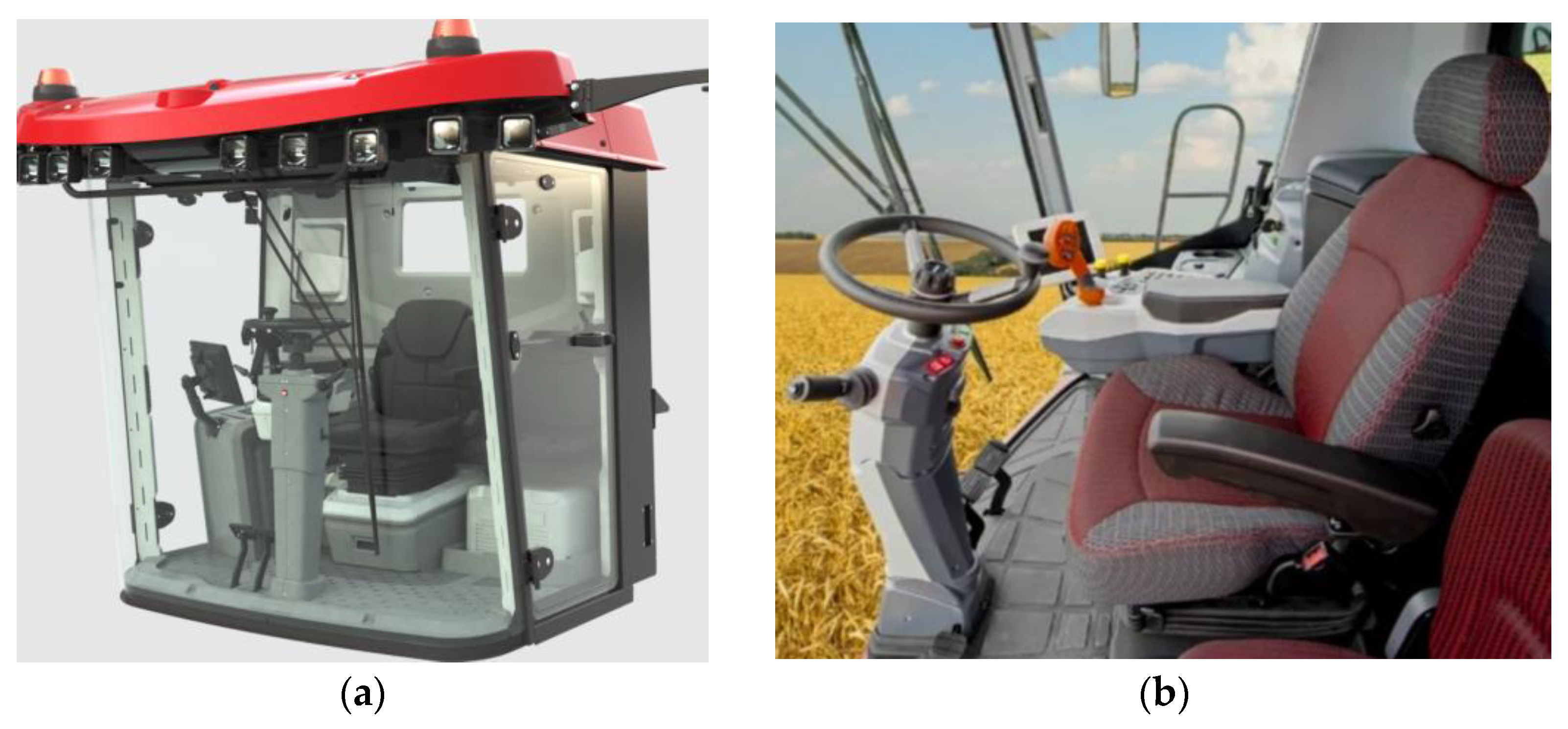
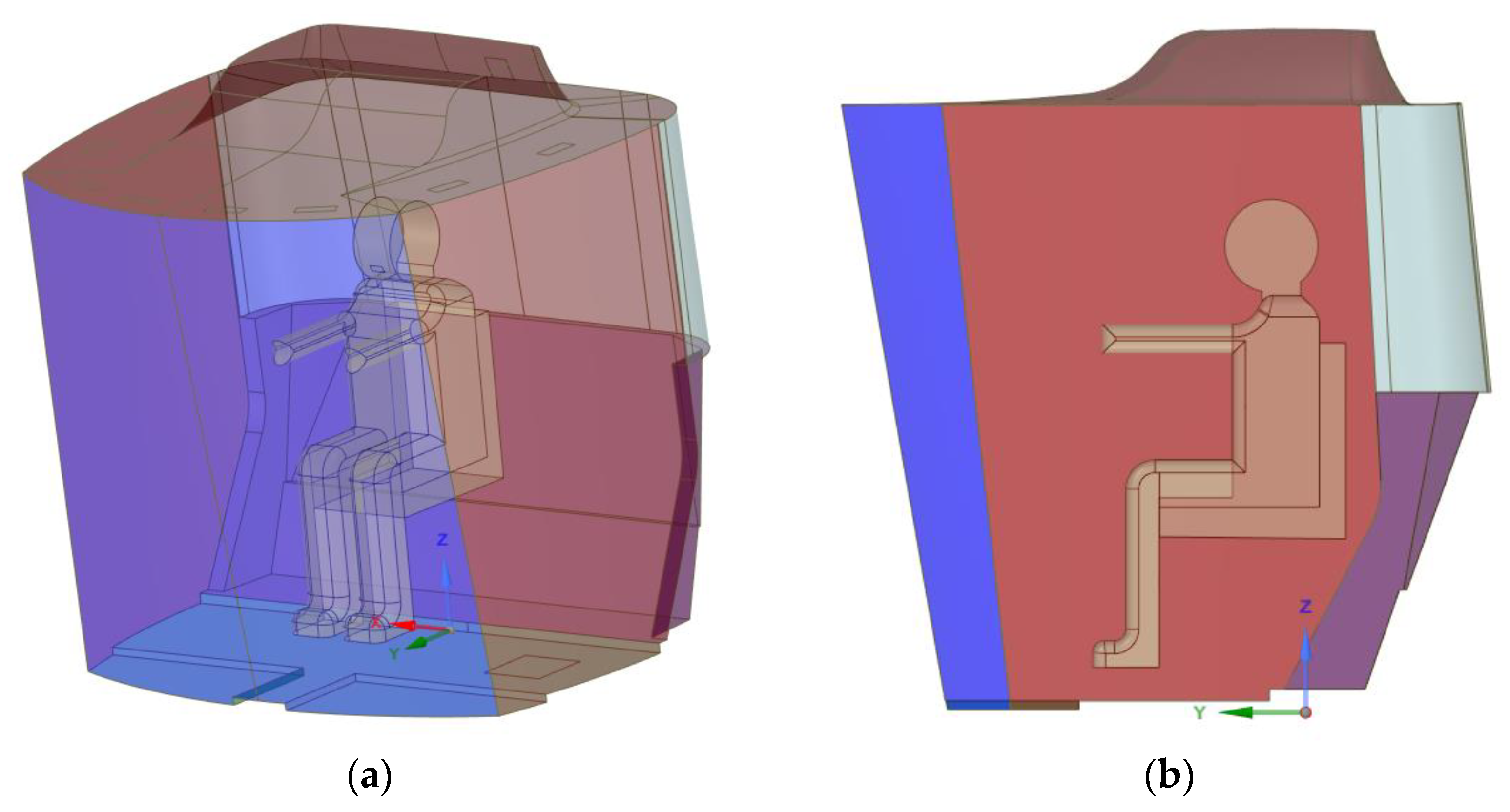
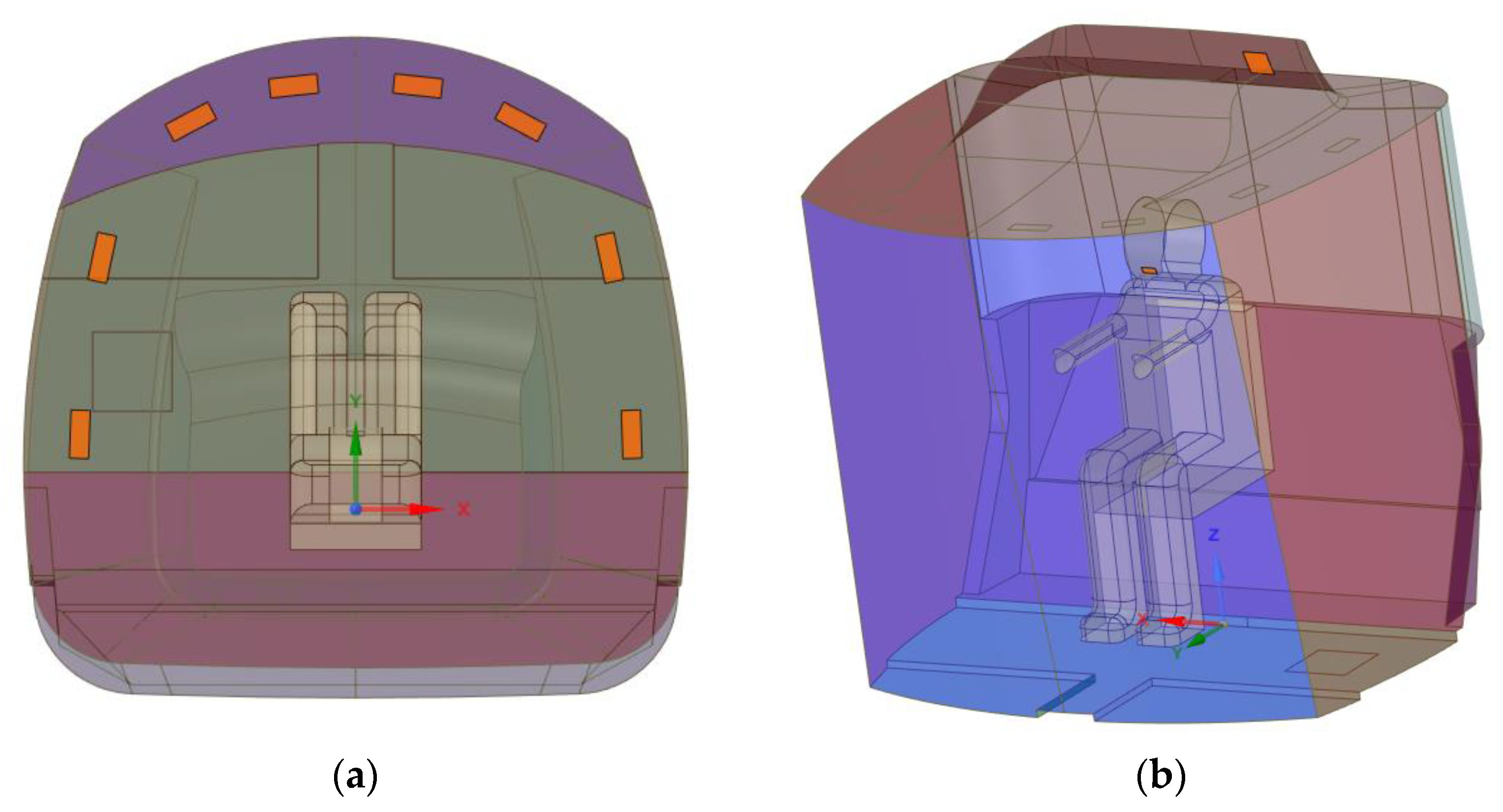
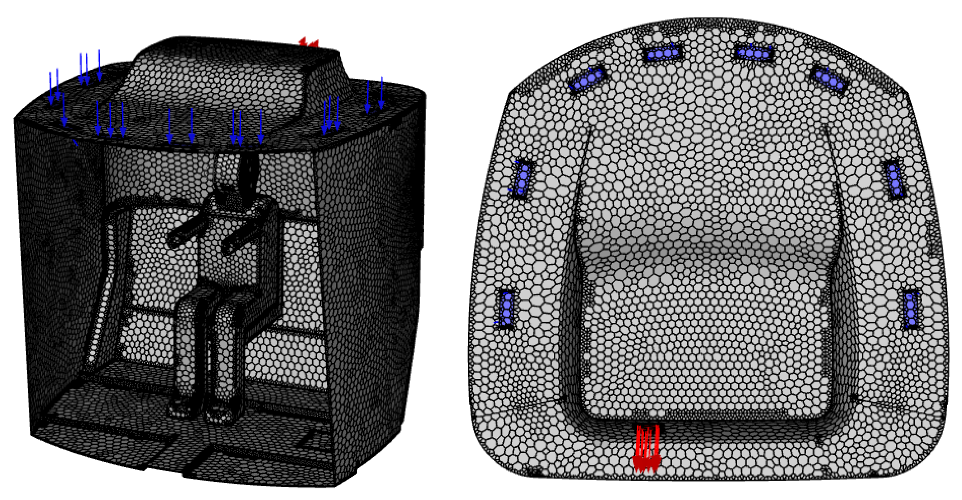
Along the boundaries of the rigid body region Ω, the conditions for zero velocities are set:

$${\mathit{u}}_n{|}_{\mathsf{\Omega }}=0, {\mathit{u}}_{\tau }{|}_{\mathsf{\Omega }}=0,$$

(20)

Here, u_n and u_τ are the normal and tangential components of the velocity vector u.

Velocity profiles (values) are set at the input:

$$\mathit{u}={\mathit{u}}^{*}.$$

(21)

Pressure values are set at the outlet:

$$p=p^{*}$$

(22)

In the numerical simulation, equations take into account the pressure relative to the reference atmospheric pressure [29,33,64,65,66,67].

Additionally, “artificial” boundary conditions are added at the outputs in the form of equality of velocity profiles or velocity derivatives in some directions, since Equation (1) contains second derivatives of velocity.

For the equation of energy and diffusion at the boundary, inlets and outlets Ω, the values of temperatures, heat fluxes, or convective heat transfer (23) are set:

$$T{|}_{\mathsf{\Omega }}=T^{*},-\lambda \frac{\partial T}{\partial n}{|}_{\mathsf{\Omega }}=q^{*}=-\alpha \left(T-T_{out}\right).$$

(23)

For diffusion, the boundary conditions are set similarly to thermal boundary conditions (23) in the form of values of concentrations, fluxes, or convective exchange at the boundaries:

$$Y_i{|}_{\mathsf{\Omega }}=Y_i{}^{*},-\frac{\partial Y_i}{\partial n}{|}_{\mathsf{\Omega }}={\mathit{J}}_i{}^{*}.$$

(24)

For particles at the inputs, the velocities, temperatures, and mass flow of particles of a certain size are set.

On the walls in this work, for particles, the boundary condition of the “trap” is set when the particle is removed from the calculation when it touches the wall.

To solve non-stationary equations in a dynamic statement, the initial values of all variables are given.

Therefore, Equations (1)–(19) together with the boundary and initial conditions (20)–(24) form a closed boundary value task of differential equations for velocities u, pressure p, temperature T, and concentrations Y_i, and coordinates and masses (diameters) of particles.

For the boundary conditions of the driver’s body surface for velocities, the standard no-slip conditions (equal to zero velocities) were used, as for ordinary walls. To simulate particles when they hit the human body, the “trap” boundary condition was used, i.e., particles were removed from the calculation.

2.4. Geometry

Figure 2 shows a diagram of a typical tractor cab. Air enters the cabin through deflectors on the roof at a given speed, temperature, and humidity, and characteristics for pathogen particles (Figure 3a). The outlet at the top rear of the cabin is set to zero relative pressure (Figure 3b). Additionally, the oral cavity of the driver can be taken into account as sources of viruses (Figure 3b).

3. Results

3.1. Numerical Analysis

To implement the numerical method for solving the equations of hydrodynamics, the fields of quantities are averaged according to Reynolds [29,33,64,65,66,67]:

$$f=\overline{f}+f^{\prime },$$

(25)

Here, $\overline{f}=\frac{1}{T}{{\displaystyle \int }}_{t-T/2}^{t+T/2}f\left(\tau \right)d\tau ,\mathrm{a}{f}^{\prime }$ is an oscillation component.

After substituting the averaged fields into the basic equations, systems of differential equations are obtained with respect to the averaged fields, as well as with respect to additional new turbulence parameters (RANS). To obtain a numerical solution for the RANS equations, Ansys Fluent is used using the k-ω turbulence model, as it is the most universal one [29,33,64,65,66,67].

The RANS approach for these flow velocities gives fairly accurate results at a relatively small grid resolution and time step and allows us to obtain a solution at lower computational costs than, for example, the LES approach [29].

The equations are solved by the finite volume method, using a pressure-based solver and the coupled method to couple velocity and pressure [29].

Figure 4 shows a finite volume mesh of 308,944 polyhedral cells and 1,008,693 nodes with six near-wall layers to account for the gradient of edge effects.

The minimum cell area is 2.1 × 10⁻⁷ m², the maximum is 2.7 × 10⁻³ m².

The mesh orthogonality is 0.16, which is sufficient for similar problems [29].

The value of the minimum residuals for the parameters of the problem is 1 × 10⁻⁴.

3.2. Task Parameters

Cabin wall is a multilayer structure with the following thermal conductivity coefficients:

Based on Formulas (26)–(28) and

Table 1. Composite wall options.

Material of the Wall	Coefficient of Thermal Conductivity, W/(m·K)	Thickness, m
Steel	58	0.002
Bituminous mastic layer	0.27	0.0042
Cast polyurethane	0.32	0.025

, the heat transfer coefficient for the walls is 5.6 W/(m²·K) and the thickness is 0.0312 m.

$$R={{\displaystyle \sum }}^{}\frac{{\delta }_i}{{\lambda }_i}+\frac{1}{{\alpha }_{out}},$$

(26)

$${\alpha }_{out}=5+3.4u^{\prime },$$

(27)

$$\alpha =\frac{1}{R}.$$

(28)

Here, R is the coefficient of thermal resistance, δ_i and λ_i are the thickness and thermal conductivity of the i-th wall, α is the thermal conductivity coefficient for the walls, and α_out are the external heat transfer coefficients of the medium. For Formula (27), the applied Yurgens formula [22] for the external velocity is used u’ = 2 m/s.

The front wall is made of laminated glass and the heat transfer coefficient is 10.9 W/(m²·K) for thickness 6 mm.

The bottom wall (floor) is thermally insulated.

Boundary conditions and air parameters are given in

Table 2. Boundary conditions and environment parameters.

Num	Title		Value
1	Incoming flow temperature, °C		30
2	Air speed in deflectors, m/s		1
3	Cabin air flow temperature, °C		14
4	Average temperature on the human surface, °C		25
5	Thermal conductivity of water vapor (H2O), W/(m2∙K)		0.0261
6	Molar mass of water vapor (H2O), kg/kmol		18.01
7	Heat capacity of water vapor (H2O), J/(kg∙K)		2014
8	Thermal conductivity of air, W/(m2∙K)		0.0242
9	Molar mass of air, kg/kmol		28.966
10	Heat capacity of air, J/(kg∙K)		1006.43
11	Mass fraction of water vapor (H2O), YH2O	Cabin inlet	0.0091
12		Cabin outlet	0.0091

.

The decrease in the mass fraction of water vapor in cold air due to condensation on the air conditioner evaporator, as well as the driver’s breathing, were not taken into account.

The value of relative humidity is determined by the formula:

$$\phi =\frac{p_{H2O}}{p_{H2O }^{*}}·100\%,$$

(29)

where $p_{H2O}$ is the partial pressure of water vapor and $p_{H2O}^{*}$ is the equilibrium pressure of saturated vapor.

The equilibrium pressure of saturated vapor can be represented by the Arden Buck formula for positive and negative temperatures, respectively [37]:

$$p_{H2O }^{*}=6.1121e^{\left[\frac{\left(18.678-\frac{T}{234.5}\right)·T}{257.14+T}\right]}·100,$$

(30)

$$p_{H2O }^{*}=6.1115e^{\left[\frac{\left(23.036-\frac{T}{333.7}\right)·T}{279.82+T}\right]}·100,$$

(31)

Here, T is the temperature in degrees Celsius.

Using the Mendeleev–Clapeyron law (7) for a fixed temperature, relative humidity can be expressed in terms of mass fractions of water vapor. Thus, for the mass fractions shown in Table 2 and the temperature of 14 °C, the relative humidity is 92.2%.

To solve the equations considering particles, it is necessary to unambiguously know the initial particle diameters of respiratory bioaerosols, the velocities, and the number of particles. At the same time, the range of particle sizes can differ significantly depending on external conditions, and the study of this issue is the topic of separate studies. In this paper, the particle size is in the range of 2 to 2000 microns according to the Rosin–Rammler distribution [29] (

Table 3. Particle parameters.

Num	Name of Injection	Deflectors	Driver’s Mouth/Cough
1	Minimum diameter value, µm	2	2
2	Maximum value of diameter, microns	2000	2000
3	Average value of diameter, microns	1000	1000
4	Initial speed, m/s	1	5
6	Mass of particles, kg/s	0.01	0.001

, Figure 5).

The no-slip condition was set on the walls of the cabin for drops.

3.3. Numerical Results

At the beginning, a non-stationary task was solved and fields of the main quantities were determined. The initial temperature inside the cabin was set to 30 °C and the mass fraction of water vapor was set to 0.0091, which corresponds to a relative humidity of 34.7%.

The time for the process to reach a stable regime was approximately 250 s. The average temperature in the cabin after 250 s was 20.2 °C and in front of the driver’s face was 20 °C, Figure 6. The average humidity in the cabin was 61.8% and in front of the driver’s face was 62.5, Figure 7.

Figure 8, Figure 9, Figure 10 and Figure 11 show the fields of velocities, pressures, temperatures, densities, and air humidity. The lines reflect the velocity trajectories, the colors reflect the values of the corresponding fields.

The fields of velocities and temperatures are unevenly distributed over the cabin volume. The minimum air temperature is 14 °C, the maximum above the walls is 29 °C. Relative humidity values in the cabin are in the range of 38.3–92.3%.

The position of the deflectors and the vertical direction of the flows cause active airflow and a relatively low temperature on the windshield.

Numerical simulation allows us to perform a series of virtual tests and choose the optimal configuration of deflectors and airflow parameters on them.

The results for the particles are shown in the following graphs below for a stabilized flow (Figure 12 and Figure 13). The colors on the value scale correspond to the size of the particle diameters. For the left graphs, the evaporation of droplets was taken into account, for the right, it was not taken into account, which corresponds with the behavior of pathogen particles in the solid state, and not in the form of aerosol droplets.

4. Discussion

From the results of the particle trajectories in Figure 12 and Figure 13, the following patterns can be noted:

➢

“Large” droplets, with a diameter greater than approximately 400 μm, hit the wall and are removed from the calculation in accordance with the sticking condition on the walls of the cabin.

➢

“Small” droplets with a diameter of more than 400 μm, in the case of taking into account the volatility of droplets, evaporate almost instantly.

If the volatility of droplets is not taken into account, “small” droplets propagate through the cabin along the streamline of air velocities, which corresponds to the behavior of pathogen particles in the solid state, and not in the form of aerosol droplets.

To analyze the particle removal rate in this case, a numerical experiment was carried out and the aerosol injection time was 0.1 with a mass of 0.01 kg/s and the distribution shown in Figure 5.

Visually, the results are presented in Figure 14. The dependences of the mass concentration and the number of particles (the number of parcels [29]) are presented in Figure 15 and Figure 16.

After 50 s, the number of particles was 10% of the maximum value and the mass fraction of particles was less than 1% after 0.2 s. This discrepancy between the mass and the quantity in part is explained by the settling of large drops on the walls of the cabin (Figure 15 and Figure 16).

The numerical results in the fields of velocities, pressures, and densities of this study were compared with the results of [22], where a study was also carried out using RANS equations without moisture and particles but taking into account the total external air domain. Figure 17 shows the temperature values in the central part of the cabin from time to time for these incoming flows specified in [22]. As can be seen from the graph, the temperature differs slightly, and the differences are probably due to the humidity in the current model.

5. Conclusions

In this study, numerical–analytical modeling of the thermal state of the vehicle interior is performed, taking into account air diffusion.

A model is also presented, which is a mathematical model of the spread of viral particles in the passenger compartment, the source of which can be air intake deflectors, as well as the operator’s respiratory tract.

• The mathematical model is implemented on the basis of the Navier–Stokes hydrodynamic equations for an ideal gas together with a discrete-element model for modeling particles with a virus in the air. The Euler–Lagrange approach is used to simulate liquid droplets in a flow. In this case, the liquid phase is considered as a continuous medium using the Navier–Stokes equations, the continuity equation, the energy equation, and the diffusion equation. Accounting for diffusion makes it possible to explicitly model air humidity and is necessary, among other things, to consider the evaporation of droplets (changes in the mass and size of particles containing the virus). The discrete-phase DPM model is used to simulate liquid drops.
• The validation of the proposed model was carried out at the stage of debugging the program in comparison with the known theoretical models of a stable flow. The results were obtained on a grid with an orthogonality of 0.16 and minimal residuals of 1 × 10⁻⁴. In addition, the comparison with previous studies of other researchers was made.
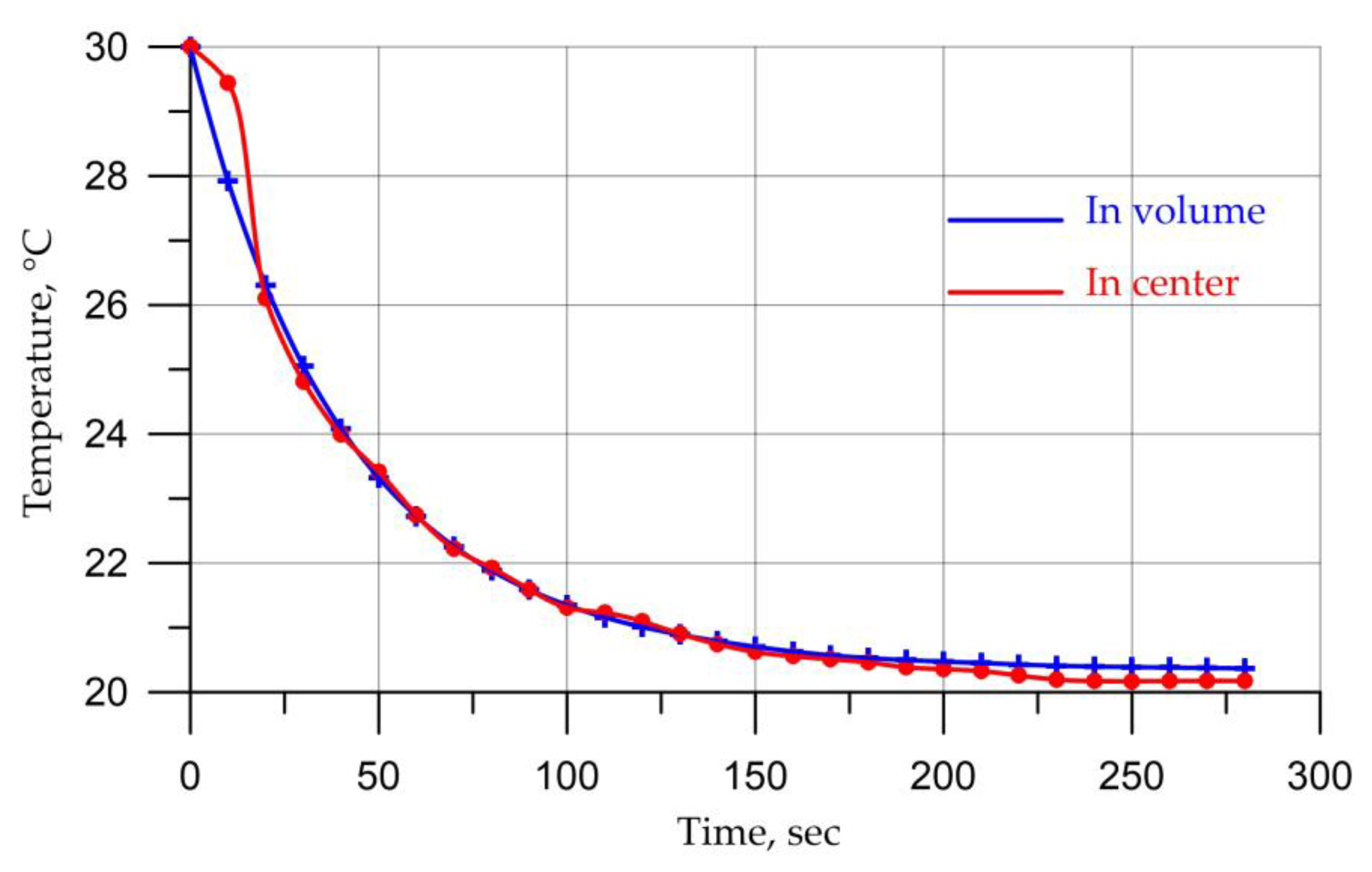
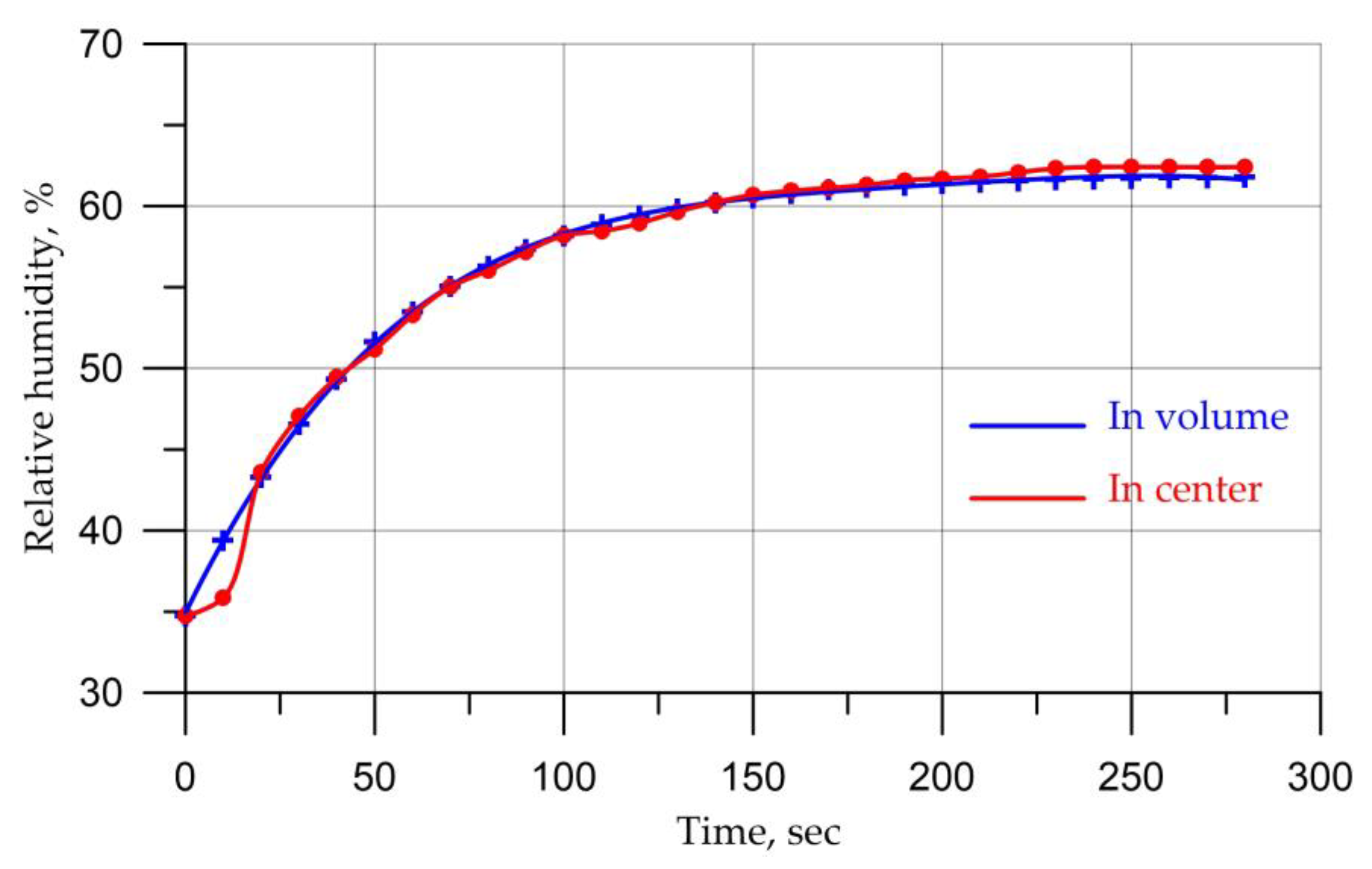
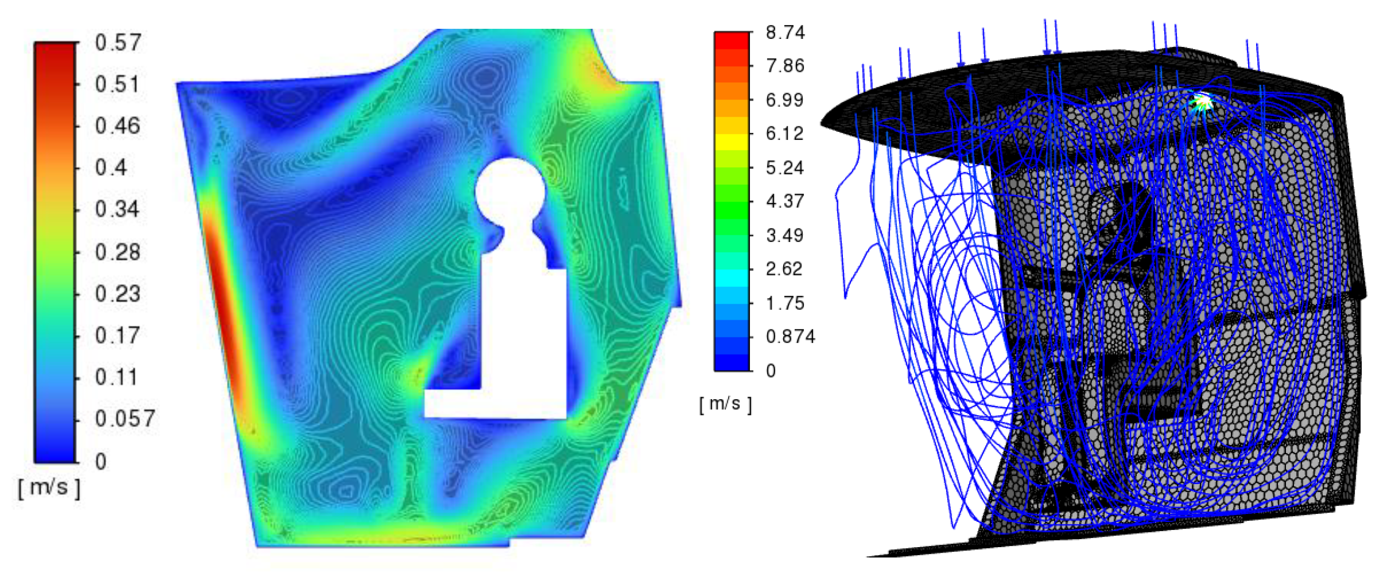
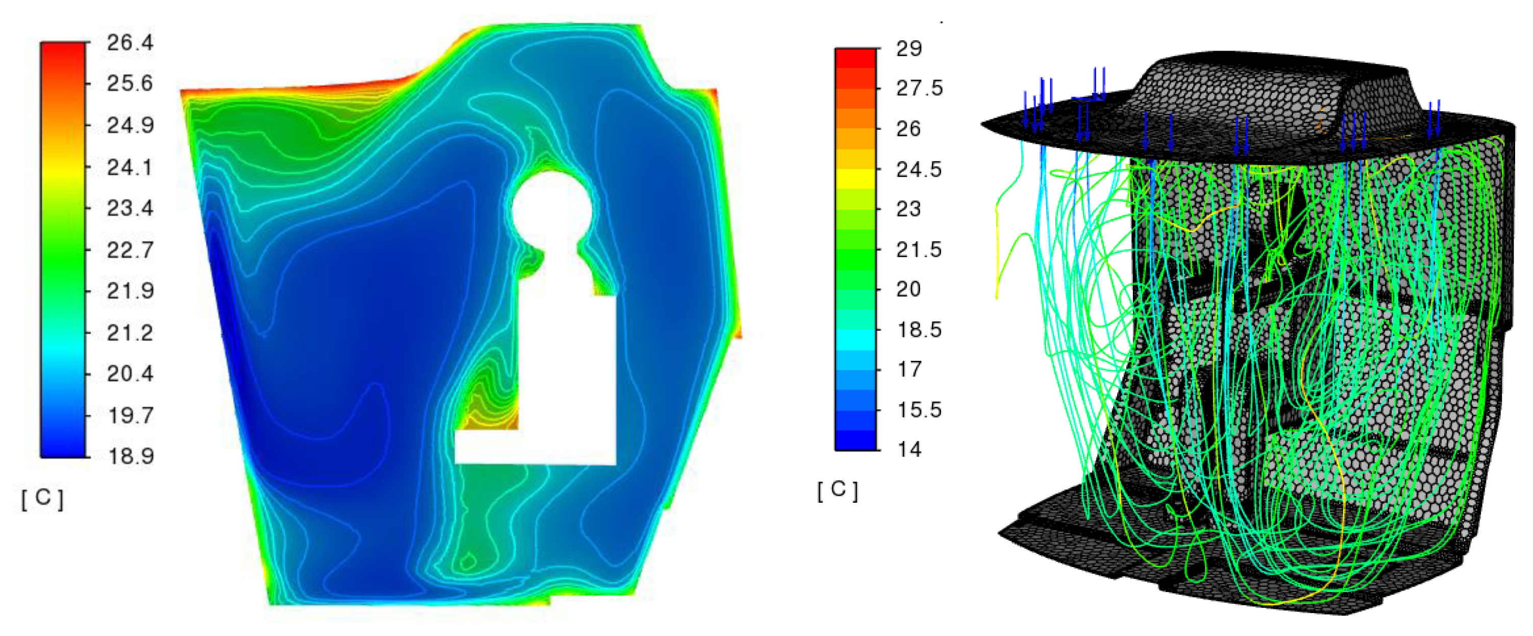
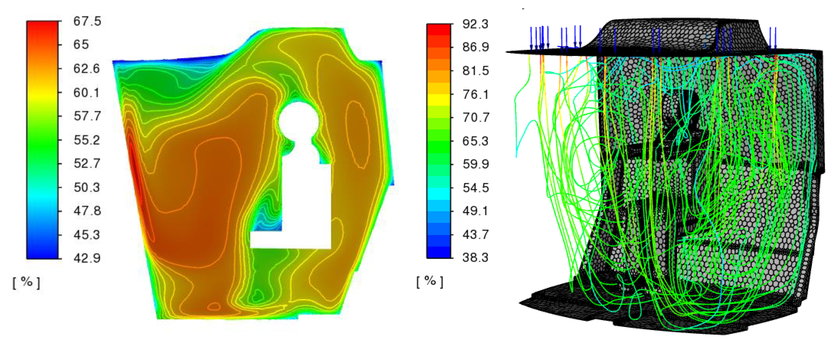
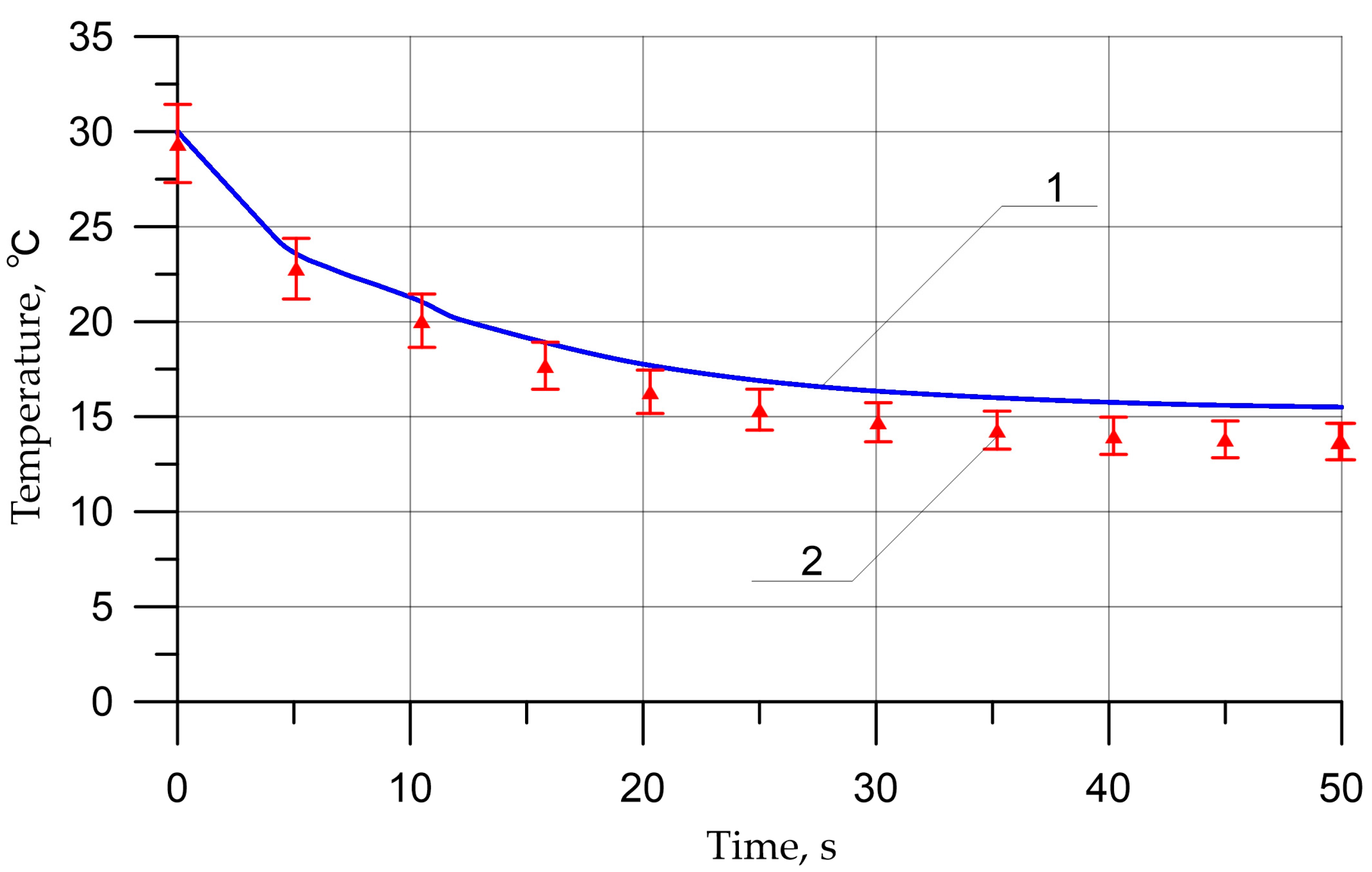
• In the work, the simulation of the fields of velocities, pressures, temperatures, and humidity in the time domain for various modes was performed. Field stabilization times were found.
• To simulate droplets containing a virus, a discrete-phase DPM model was used, for which the discrete and continuous phases are interconnected through the initial terms in the equations. The following regularities were found:
• “Large” drops, with a diameter greater than approximately 400 microns, hit the wall and were removed from the calculation in accordance with the sticking condition on the walls of the cabin.
• “Small” droplets, with a diameter of more than 400 microns, in the case of taking into account the evaporation of droplets, evaporate almost instantly.
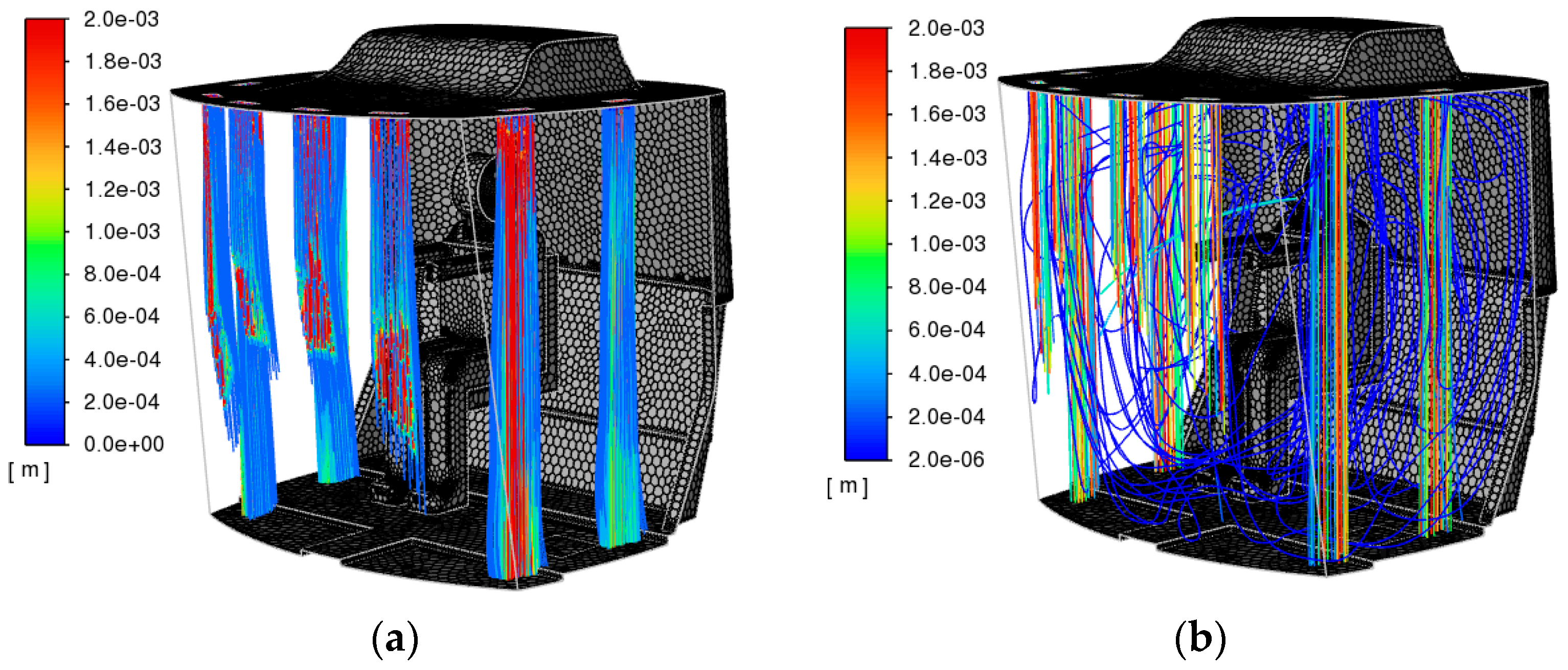
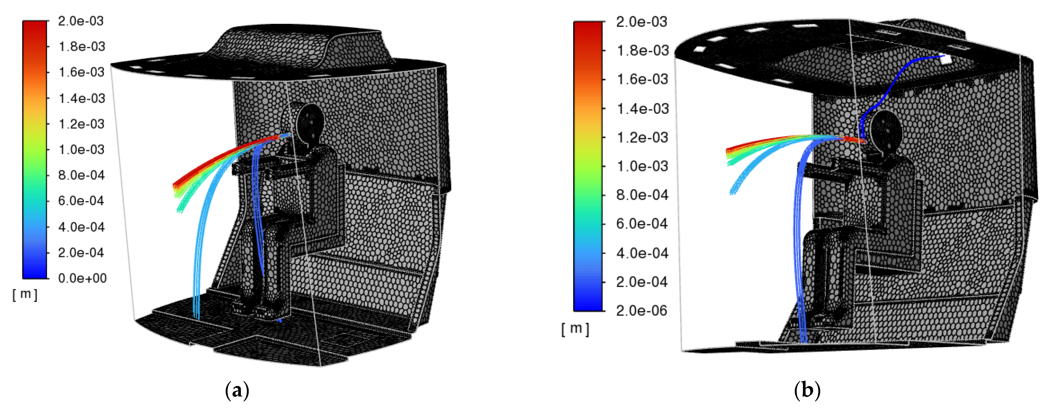
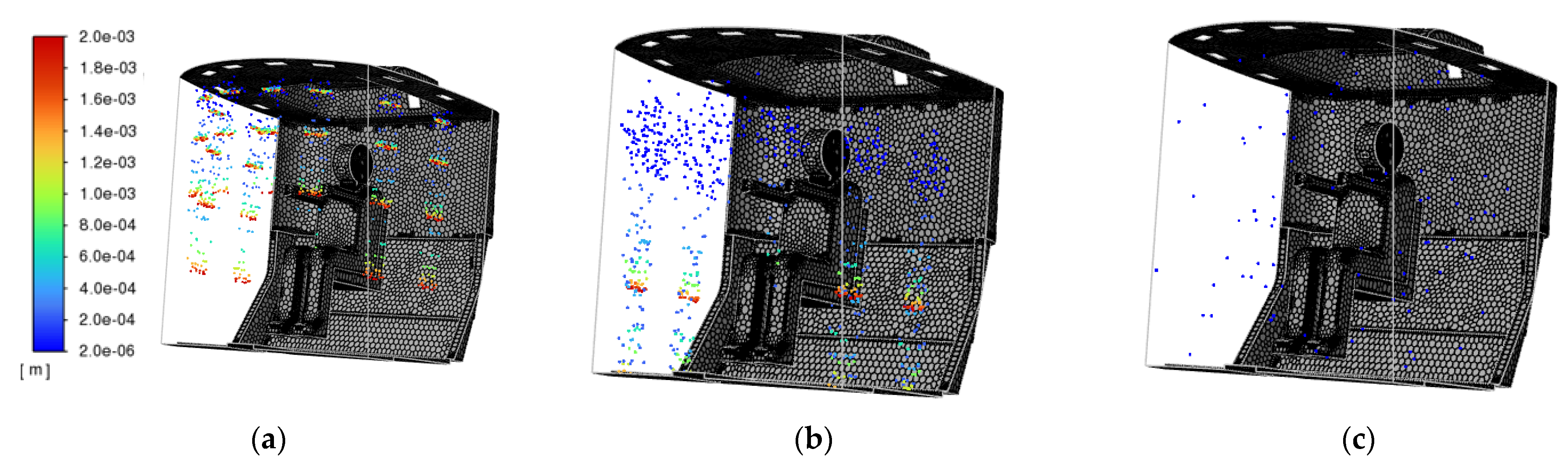
• “Small” droplets, with a diameter of more than 400 μm, in the case of non-evaporability of droplets, propagate through the cabin along the streamline of air velocities, and the dependences of concentrations and the number of particles in the cabin on time are plotted.
• In this work, only one value of air humidity was considered: “non-evaporable” particles. It is also quite interesting to study the influence of the humidity value on the evaporation of particles, and therefore on their behavior in the volume of the cabin. In addition, the question of the influence of the airflow directions of the air deflectors of the climate system and the internal equipment of the cabin remains unexplored. These studies, field tests and comparison of the results are planned to be carried out in subsequent works.

This fact confirms the need for further study of the nature of the spread of viruses and pathogens in respiratory droplets and in solid states.

This approach is universal and can be used to simulate the thermal state, considering the humidity of cabins and the climatic equipment of any configuration.

The presented model makes it possible to study the spread of pathogens that are inside respiratory droplets or in solid form, and to predict the time of removal of pathogens from the cockpit.

References

1. Mikhailov, M.V.; Guseva, S.V. Microclimate in the Cabins of Mobile Vehicles; Engineering: Moscow, Russia, 1977; 230p. [Google Scholar]
2. Panfilov, I.A.; Soloviev, A.N.; Matrosov, A.A.; Meskhi, B.C.; Polushkin, O.O.; Rudoy, D.V.; Pakhomov, V.I. Finite element sim-ulation of airflow in a field cleaner. IOP Conf. Ser. Mater. Sci. Eng. 2020, 1001, 012060. [Google Scholar] [CrossRef]
3. Loitsyansky, L.G. Mechanics of Liquid and Gas: Studies for Universities, 7th ed.; ISPR: Rawalpindi, Pakistan; Drofa: Moscow, Russia, 2003.
4. Bhagat, R.K.; Davies Wykes, M.S.; Dalziel, S.B.; Linden, P.F. Effects of ventilation on the indoor spread of COVID-19. J. Fluid Mech. 2020, 903, F1. [Google Scholar] [CrossRef] [PubMed]
5. Meskhi, B.; Rudoy, D.; Lachuga, Y.; Pakhomov, V.; Soloviev, A.; Matrosov, A.; Panfilov, I.; Maltseva, T. Finite Element and Applied Models of the Stem with Spike Deformation. Agriculture 2021, 11, 1147. [Google Scholar] [CrossRef]
6. Fabregat, A.; Gisbert, F.; Vernet, A.; Dutta, S.; Mittal, K.; Pallarès, J. Direct numerical simulation of the turbulent flow generated during a violent expiratory event. Phys. Fluids 2021, 33, 035122. [Google Scholar] [CrossRef]
7. Katre, P.; Banerjee, S.; Balusamy, S.; Sahu, K.C. Fluid dynamics of respiratory droplets in the context of COVID-19: Airborne and surfaceborne transmissions. Phys. Fluids 2021, 33, 081302. [Google Scholar] [CrossRef] [PubMed]
8. Baehr, H.D.; Kabelac, S. Thermodynamik; Springer: Berlin/Heidelberg, Germany, 2012; 667p. [Google Scholar] [CrossRef]
9. Bazarov, I.P. Thermodynamics; Higher School: Moscow, Russia, 1983; 341p. [Google Scholar]
10. Kuzovlev, V.A. Technical Thermodynamics and Basics of Heat Transfer, 2nd ed.; Higher School: Moscow, Russia, 1983; 335p. [Google Scholar]
11. Soloviev, A.N.; Oganesyan, P.A.; Skaliukh, A.S.; Duong, L.V.; Gupta, V.K.; Panfilov, I.A. Comparison between applied theory and final element method for energy harvesting non-homogeneous piezoelements modeling. In Advanced Materials; Springer Proceedings in Physics; Springer: Cham, Switzerland, 2017; Volume 193, pp. 473–484. [Google Scholar] [CrossRef]
12. Karthick, L.; Prabhu, D.; Rameshkumar, K.; Prabhu, T.; Jagadish, C.A. CFD analysis of rotating diffuser in a SUV vehicle for improving thermal comfort. Mater. Today Proc. 2022, 52, 1014–1025. [Google Scholar] [CrossRef]
13. Hemmati, S.; Doshi, N.; Hanover, D.; Morgan, C.; Shahbakhti, M. Integrated cabin heating and powertrain thermal energy management for a connected hybrid electric vehicle. Appl. Energy 2021, 283, 116353. [Google Scholar] [CrossRef]
14. Panfilov, I.A.; Ustinov, Y.A. Harmonic vibrations and waves in a cylindrical helically anisotropic shell. Mech. Solids 2012, 47, 195–204. [Google Scholar] [CrossRef]
15. Bandi, P.; Manelil, N.P.; Maiya, M.P.; Tiwari, S.; Thangamani, A.; Tamalapakula, J.L. Influence of flow and thermal characteristics on thermal comfort inside an automobile cabin under the effect of solar radiation. Appl. Therm. Eng. 2022, 203, 117946. [Google Scholar] [CrossRef]
16. Tan, L.; Yuan, Y. Computational fluid dynamics simulation and performance optimization of an electrical vehicle Air-conditioning system. Alex. Eng. J. 2022, 61, 315–328. [Google Scholar] [CrossRef]
17. Beskopylny, A.; Kadomtseva, E.; Strelnikov, G. Numerical study of the stress-strain state of reinforced plate on an elastic foundation by the Bubnov-Galerkin method. IOP Conf. Ser. Earth Environ. Sci. 2017, 90, 012017. [Google Scholar] [CrossRef]
18. Singh, S.; Abbassi, H. 1D/3D transient HVAC thermal modeling of an off-highway machinery cabin using CFD-ANN hybrid method. Appl. Therm. Eng. 2018, 135, 406–417. [Google Scholar] [CrossRef]
19. Chang, T.-B.; Sheu, J.-J.; Huang, J.-W.; Lin, Y.-S.; Chang, C.-C. Development of a CFD model for simulating vehicle cabin indoor air quality. Transp. Res. Part D Transp. Environ. 2018, 62, 433–440. [Google Scholar] [CrossRef]
20. Ahmed Mboreha, C.; Jianhong, S.; Yan, W.; Zhi, S.; Yantai, Z. Investigation of thermal comfort on innovative personalized ventilation systems for aircraft cabins: A numerical study with computational fluid dynamics. Therm. Sci. Eng. Prog. 2021, 26, 101081. [Google Scholar] [CrossRef]
21. Oh, J.; Choi, K.; Son, G.; Park, Y.-J.; Kang, Y.-S.; Kim, Y.-J. Flow analysis inside tractor cabin for determining air conditioner vent location. Comput. Electron. Agric. 2020, 169, 105199. [Google Scholar] [CrossRef]
22. Beskopylny, A.N.; Panfilov, I.; Meskhi, B. Modeling of Flow Heat Transfer Processes and Aerodynamics in the Cabins of Vehicles. Fluids 2022, 7, 226. [Google Scholar] [CrossRef]
23. Kaewbumrung, M.; Charoenloedmongkhon, A. Numerical Simulation of Turbulent Flow in Eccentric Co-Rotating Heat Transfer. Fluids 2022, 7, 131. [Google Scholar] [CrossRef]
24. Abdel Aziz, S.S.; Saber Salem Said, A.-H. Numerical Investigation of Flow and Heat Transfer over a Shallow Cavity: Effect of Cavity Height Ratio. Fluids 2021, 6, 244. [Google Scholar] [CrossRef]
25. Lahaye, D.; Nakate, P.; Vuik, K.; Juretić, F.; Talice, M. Modeling Conjugate Heat Transfer in an Anode Baking Furnace Using OpenFoam. Fluids 2022, 7, 124. [Google Scholar] [CrossRef]
26. Beskopylny, A.; Chukarin, A.; Meskhi, B.; Isaev, A. Modeling of Vibroacoustic Characteristics of Plate Structures of Vehicles during Abrasive Processing. Transp. Res. Procedia 2021, 54, 39–46. [Google Scholar] [CrossRef]
27. Lv, X.; Wu, W.-T.; Lv, J.; Mao, K.; Gao, L.; Li, Y. Study on the Law of Pseudo-Cavitation on Superhydrophobic Surface in Turbulent Flow Field of Backward-Facing Step. Fluids 2021, 6, 200. [Google Scholar] [CrossRef]
28. Vlasov, M.N.; Merinov, I.G. Application of an Integral Turbulence Model to Close the Model of an Anisotropic Porous Body as Applied to Rod Structures. Fluids 2022, 7, 77. [Google Scholar] [CrossRef]
29. ANSYS Inc. Fluent User’s Guide: Release 2022 R1 January 2022; ANSYS Inc.: Canonsburg, PA, USA, 2022; Available online: http://www.pmt.usp.br/academic/martoran/notasmodelosgrad/ANSYS%20Fluent%20Users%20Guide.pdf (accessed on 27 December 2022).
30. Caccavale, P.; Mele, B.; Brandizzi, M.; Ruocco, G. Fully Coupled Fluid–Structure Interaction with Heat Transfer Effects in an Adaptive NACA Airfoil. Fluids 2023, 8, 39. [Google Scholar] [CrossRef]
31. Xu, X.; Huang, X.; Bi, D.; Zhou, M. A Combined Artificial-Intelligence Aerodynamic Design Method for a Transonic Compressor Rotor Based on Reinforcement Learning and Genetic Algorithm. Appl. Sci. 2023, 13, 1026. [Google Scholar] [CrossRef]
32. Zhang, M.; Hao, S.; Hou, A. Study on the Intelligent Modeling of the Blade Aerodynamic Force in Compressors Based on Machine Learning. Mathematics 2021, 9, 476. [Google Scholar] [CrossRef]
33. Pope, S. Turbulent Flows; Cambridge University Press: Cambridge, UK, 2000; 771p. [Google Scholar] [CrossRef]
34. Habchi, C.; Oneissi, M.; Russeil, S.; Bougeard, D.; Lemenand, T. Comparison of eddy viscosity turbulence models and stereoscopic PIV measurements for a flow past rectangular-winglet pair vortex generator. Chem. Eng. Process.-Process Intensif. 2021, 169, 108637. [Google Scholar] [CrossRef]
35. Bauer, J.; Tyacke, J. Comparison of low Reynolds number turbulence and conjugate heat transfer modelling for pin-fin roughness elements. Appl. Math. Model. 2022, 103, 696–713. [Google Scholar] [CrossRef]
36. Erb, A.; Hosder, S. Analysis and comparison of turbulence model coefficient uncertainty for canonical flow problems. Comput. Fluids 2021, 227, 105027. [Google Scholar] [CrossRef]
37. Sukhinov, A.; Belova, Y.; Chistyakov, A.; Beskopylny, A.; Meskhi, B. Mathematical Modeling of the Phytoplankton Populations Geographic Dynamics for Possible Scenarios of Changes in the Azov Sea Hydrological Regime. Mathematics 2021, 9, 3025. [Google Scholar] [CrossRef]
38. Lyapin, A.; Beskopylny, A.; Meskhi, B. Structural Monitoring of Underground Structures in Multi-Layer Media by Dynamic Methods. Sensors 2020, 20, 5214. [Google Scholar] [CrossRef]
39. Broatch, A.; Olmeda, P.; Plá, B.; Dreif, A.; Onorati, A.; Marinoni, A. Numerical assessment of integrated thermal management systems in electrified powertrains. Appl. Therm. Eng. 2023, 221, 119822. [Google Scholar] [CrossRef]
40. Steinstraeter, M.; Buberger, J.; Minnerup, K.; Trifonov, D.; Horner, P.; Weiss, B.; Lienkamp, M. Controlling cabin heating to improve range and battery lifetime of electric vehicles. eTransportation 2022, 13, 100181. [Google Scholar] [CrossRef]
41. Lei, S.; Xin, S.; Liu, S. Separate and integrated thermal management solutions for electric vehicles: A review. J. Power Sources 2022, 550, 232133. [Google Scholar] [CrossRef]
42. Beskopylny, A.N.; Meskhi, B.; Stel’makh, S.A.; Shcherban’, E.M.; Mailyan, L.R.; Veremeenko, A.; Akopyan, V.; Shilov, A.V.; Chernil’nik, A.; Beskopylny, N. Numerical Simulation of the Bearing Capacity of Variotropic Short Concrete Beams Reinforced with Polymer Composite Reinforcing Bars. Polymers 2022, 14, 3051. [Google Scholar] [CrossRef]
43. Chang, T.; Lin, Y.; Hsu, Y. CFD simulations of effects of recirculation mode and fresh air mode on vehicle cabin indoor air quality. Atmos. Environ. 2023, 293, 119473. [Google Scholar] [CrossRef]
44. Beskopylny, A.N.; Stel’makh, S.A.; Shcherban’, E.M.; Mailyan, L.R.; Meskhi, B.; Efremenko, I.; Varavka, V.; Beskopylny, N.; Dotsenko, N. Modeling and Experimental Verification of the Performance of Polymer Composite Reinforcing Bars of Different Types in Concrete of Different Density. Polymers 2022, 14, 1756. [Google Scholar] [CrossRef] [PubMed]
45. Shcherban’, E.M.; Stel’makh, S.A.; Beskopylny, A.; Mailyan, L.R.; Meskhi, B.; Shuyskiy, A.; Beskopylny, N.; Dotsenko, N. Mathematical Modeling and Experimental Substantiation of the Gas Release Process in the Production of Non-Autoclaved Aerated Concrete. Materials 2022, 15, 2642. [Google Scholar] [CrossRef]
46. Hassan, A.M.; Megahed, N.A. COVID-19 and urban spaces: A new integrated CFD approach for public health opportunities. Build. Environ. 2021, 204, 108131. [Google Scholar] [CrossRef] [PubMed]
47. Motamedi, H.; Shirzadi, M.; Tominaga, Y.; Mirzaei, P.A. CFD modeling of airborne pathogen transmission of COVID-19 in confined spaces under different ventilation strategies. Sustain. Cities Soc. 2022, 76, 103397. [Google Scholar] [CrossRef]
48. Faleiros, D.E.; van den Bos, W.; Botto, L.; Scarano, F. TU Delft COVID-app: A tool to democratize CFD simulations for SARS-CoV-2 infection risk analysis. Sci. Total Environ. 2022, 826, 154143. [Google Scholar] [CrossRef]
49. Alrebi, O.F.; Obeidat, B.; Abdallah, I.A.; Darwish, E.F.; Amhamed, A. Airflow dynamics in an emergency department: A CFD simulation study to analyse COVID-19 dispersion. Alex. Eng. J. 2022, 61, 3435–3445. [Google Scholar] [CrossRef]
50. Mirzaie, M.; Lakzian, E.; Khan, A.; Warkiani, M.E.; Mahian, O.; Ahmadi, G. COVID-19 spread in a classroom equipped with partition—A CFD approach. J. Hazard. Mater. 2021, 420, 126587. [Google Scholar] [CrossRef] [PubMed]
51. Bahramian, A.; Mohammadi, M.; Ahmadi, G. Effect of indoor temperature on the velocity fields and airborne transmission of sneeze droplets: An experimental study and transient CFD modeling. Sci. Total Environ. 2023, 858, 159444. [Google Scholar] [CrossRef] [PubMed]
52. Sarhan, A.A.R.; Naser, P.; Naser, J. Aerodynamic Prediction of Time Duration to Becoming Infected with Coronavirus in a Public Place. Fluids 2022, 7, 176. [Google Scholar] [CrossRef]
53. Li, R.; Liu, G.; Xia, Y.; Bantserova, O.L.; Li, W.; Zhu, J. Pollution Dispersion and Predicting Infection Risks in Mobile Public Toilets Based on Measurement and Simulation Data of Indoor Environment. Processes 2022, 10, 2466. [Google Scholar] [CrossRef]
54. Ren, J.; Duan, S.; Guo, L.; Li, H.; Kong, X. Effects of Return Air Inlets’ Location on the Control of Fine Particle Transportation in a Simulated Hospital Ward. Int. J. Environ. Res. Public Health 2022, 19, 11185. [Google Scholar] [CrossRef] [PubMed]
55. Al-Rawi, M.; Al-Jumaily, A.M.; Lazonby, A. Did You Just Cough? Visualization of Vapor Diffusion in an Office Using Computational Fluid Dynamics Analysis. Int. J. Environ. Res. Public Health 2022, 19, 9928. [Google Scholar] [CrossRef]
56. Cheng, C.-L.; Lin, Y.-Y. CFD Numerical Simulation in Building Drainage Stacks as an Infection Pathway of COVID-19. Int. J. Environ. Res. Public Health 2022, 19, 7475. [Google Scholar] [CrossRef]
57. Rahvard, A.J.; Karami, S.; Lakzian, E. Finding the proper position of supply and return registers of air condition system in a conference hall in term of COVID-19 virus spread. Int. J. Refrig. 2023, 145, 78–89. [Google Scholar] [CrossRef]
58. Goodson, M.; Feaster, J.; Jones, A.; McGowan, G.; Agricola, L.; Timms, W.; Uddin, M. Modeling Transport of SARS-CoV-2 Inside a Charlotte Area Transit System (CATS) Bus. Fluids 2022, 7, 80. [Google Scholar] [CrossRef]
59. Wang, Z.; Galea, E.R.; Grandison, A.; Ewer, J.; Jia, F. A coupled Computational Fluid Dynamics and Wells-Riley model to predict COVID-19 infection probability for passengers on long-distance trains. Saf. Sci. 2022, 147, 105572. [Google Scholar] [CrossRef]
60. Morsi, S.A.; Alexander, A.J. An Investigation of Particle Trajectories in Two-Phase Flow Systems. J. Fluid Mech. 1972, 55, 193–208. [Google Scholar] [CrossRef]
61. Dennis, S.C.R.; Singh, S.N.; Ingham, D.B. The steady flow due to a rotating sphere at low and moderate Reynolds numbers. J. Fluid Mech. 1980, 101, 257–279. [Google Scholar] [CrossRef]
62. Miller, R.S.; Harstad, K.; Bellan, J. Evaluation of Equilibrium and Non-Equilibrium Evaporation Models for Many Droplets Gas-Liquid Flow Simulations. Int. J. Multiph. Flow 1998, 24, 1025–1055. [Google Scholar] [CrossRef]
63. Sazhin, S.S. Advanced Models of Fuel Droplet Heating and Evaporation. Prog. Energy Combust. Sci. 2006, 32, 162–214. [Google Scholar] [CrossRef]
64. Couto, N.; Bergada, J.M. Aerodynamic Efficiency Improvement on a NACA-8412 Airfoil via Active Flow Control Implementation. Appl. Sci. 2022, 12, 4269. [Google Scholar] [CrossRef]
65. Klein, M.; Trummler, T.; Urban, N.; Chakraborty, N. Multiscale Analysis of Anisotropy of Reynolds Stresses, Subgrid Stresses and Dissipation in Statistically Planar Turbulent Premixed Flames. Appl. Sci. 2022, 12, 2275. [Google Scholar] [CrossRef]
66. Yang, X.; Yang, L. An Elliptic Blending Turbulence Model-Based Scale-Adaptive Simulation Model Applied to Fluid Flows Separated from Curved Surfaces. Appl. Sci. 2022, 12, 2058. [Google Scholar] [CrossRef]
67. Ghoroghi, A.; Rezgui, Y.; Wallace, R. Impact of ventilation and avoidance measures on SARS-CoV-2 risk of infection in public indoor environments. Sci. Total Environ. 2022, 838, 156518. [Google Scholar] [CrossRef]
Figure 1. Combine harvester cab: (a) outside view and (b) inside view.
Mathematics 11 00784 g001
Figure 2. General view: (a) axonometry; (b) side view.
Mathematics 11 00784 g002
Figure 3. General scheme: (a) circuit inputs and (b) circuit output.
Mathematics 11 00784 g003
Figure 4. Mesh of finite volumes.
Mathematics 11 00784 g004
Figure 5. Distribution of particles at the entrances.
Mathematics 11 00784 g005
Figure 6. Average temperature.
Mathematics 11 00784 g006
Figure 7. Average relative humidity.
Mathematics 11 00784 g007
Figure 8. Relative pressure, Pa.
Mathematics 11 00784 g008
Figure 9. Velocity field m/s.
Mathematics 11 00784 g009
Figure 10. Temperature, °C.
Mathematics 11 00784 g010
Figure 11. Relative humidity °C.
Mathematics 11 00784 g011
Figure 12. Trajectories and diameters of pathogen particles for deflectors, the colors on the value scale correspond to the size of particle diameters (a) with volatility and (b) without volatility.
Mathematics 11 00784 g012
Figure 13. Trajectories and particle diameters of pathogens during the driver’s cough, the colors on the value scale correspond to the particle diameter size (a) with volatility and (b) without volatility.
Mathematics 11 00784 g013
Figure 14. Trajectories and diameters of pathogen particles for deflectors versus time, the colors on the scale of values correspond to the size of particle diameters: (a) time 0.4 s; (b) time 1.2 s; (c) time 127 s.
Mathematics 11 00784 g014
Figure 15. Particle concentration over time.
Mathematics 11 00784 g015
Figure 16. Number of particles over time.
Mathematics 11 00784 g016
Figure 17. Temperature in the central part of the cabin: 1—previous solution [22]; 2—new results.
Mathematics 11 00784 g017