Characteristic, C-Characteristic and Positive Cones in Hyperfields

Abstract

We study the notions of the positive cone, characteristic and C-characteristic in (Krasner) hyperfields. We demonstrate how these interact in order to produce interesting results in the theory of hyperfields. For instance, we provide a criterion for deciding whether certain hyperfields cannot be obtained via Krasner’s quotient construction. We prove that any positive integer (larger than 1) can be realized as the characteristic of some infinite hyperfield and an analogous result for the C-characteristic. Finally, we study the (directed) graph associated with the strict partial order induced by a positive cone in a hyperfield in various examples.

1. Introduction

In this paper, we study Krasner hyperfields. These structures are a generalization of the concept of the field, where the addition is allowed to be a multivalued operation, i.e., $x+y$ in general denotes a subset and not only an element. Apart from the applications for which they have been introduced in [1] by Krasner, recently, these structures have arisen naturally in several mathematical contexts. For instance, Viro in [2] used hyperfields in tropical geometry and Lee in [3] studied these structures in connection to the model theory of valued fields. Regarding hyperfields, it is certainly also worth mentioning the work of Connes and Consani in number theory [4,5].

Since hyperfields represent a generalization of the concept of a field, it is natural to ask which classical notions and theorems of the theory of fields can be generalized to the theory of hyperfields. M. Marshall in [6] started the investigation towards a theory of real hyperfields, generalizing the Artin-Schreier theory of real fields (for a general reference on the latter, we refer the reader to [7]). The work of Marshall provided the basis for the investigations made later in [8] and in [9]. In the sections below, real hyperfields will be studied further.

Historically, a subhyperfield L of a hyperfield F is required to be closed under the multivalued addition in the sense that $x+y\subseteq L$ for all $x,y\in L$. However, Jun in (Definition 2.4) [10], felt the need for a less restrictive notion and started to talk about a multivalued operation, which can be “induced” by certain subsets. In Section 3, we take a model theoretical point of view (encoding the multivalued operation + via the ternary relation $z\in x+y$) to justify Jun’s feeling and precisely define the notion of the multivalued operation induced by a subset (see also [9]). This leads us to the notion of relational subhyperfields. The interest for relational subhyperfields is motivated by the fact that they correspond to the submodels of hyperfields in a natural first-order language, which we describe in Section 3.

The notion of this characteristic is fundamental in classical field theory and, when it is finite, it can only be a prime number. Moreover, the characteristic of a field is preserved by subfields. In this paper, we will demonstrate that a natural generalization of the notion of characteristic for hyperfields (see Definition 3 below), does not have to behave in the same way: we prove that the characteristic of a hyperfield does not have to be preserved by relational subhyperfields (Example 13), and that any integer greater than 1 can be realized as the characteristic of some hyperfield (Theorem 3).

In addition, we study an alternative notion of the characteristic for hyperfields, known as the C-characteristic, which in the case of fields coincides with the usual characteristic. Moreover, this quantity is not preserved by relational subhyperfields (Example 14), and we prove in Theorem 4 that any positive integer can be realized as the C-characteristic of some real hyperfield. In addition, we demonstrate how useful the interplay between these two notions of characteristic can be by providing a criterion (Theorem 6) for deciding whather certain hyperfields cannot be obtained via Krasner’s quotient construction (see [11,12]). We apply this result to the finite real hyperfield of Example 4.

In Section 5, we define a strict partial order relation induced by a positive cone in a real hyperfield and study the associated directed graph in various interesting examples.

2. Preliminaries

In this section, we provide an overview of the definitions and facts that are necessary for the rest of the paper, with several examples.

2.1. Hyperfields

Let H be a non-empty set and $\mathcal{P}\left(H\right)$ be its power-set. A multivalued operation+ on H is a function which associates with every pair $(x,y)\in H\times H$ an element of $\mathcal{P}\left(H\right)$, denoted by $x+y$. A hyperoperation + on H is a multivalued operation, such that $x+y\ne \varnothing$ for all $x,y\in H$. If + is a multivalued operation on $H\ne \varnothing$, then for $x\in H$ and $A,B\subseteq H$, we set

$$A+B:=\bigcup _{a\in A,b\in B}a+b,$$

(1)

$A+x:=A+\left\{x\right\}$ and $x+A:=\left\{x\right\}+A$. If A or B is empty, then so is $A+B$.

A hypergroup can be defined as a non-empty set H with a multivalued operation +, which is associative (see Definition 1 (CH1) below) and reproductive (i.e., $x+H=H+x=H$ for all $x\in H$). This notion was first considered by F. Marty in [13,14,15]. Let us mention [16] for an extended historical overview and [17,18] for a description of some applications.

If $(H,+)$ is a hypergroup, then it follows that + is a hyperoperation. Indeed, suppose that $x+y=\varnothing$ for some $x,y\in H$. Then,

$$H=x+H=x+(y+H)=(x+y)+H=\varnothing +H=\varnothing ,$$

which is excluded (cf. (Theorem 12) in [16]).

The following special class of hypergroups will be of interest for us.

Definition 1.

A canonical hypergroup is a tuple $(H,+,0)$, where $H\ne \varnothing$, + is a multivalued operation on H and 0 is an element of H such that the following axioms hold:

(CH1) 

+ is associative, i.e., $(x+y)+z=x+(y+z)$ for all $x,y,z\in H$,

(CH2) 

$x+y=y+x$ for all $x,y\in H$,

(CH3) 

for every $x\in H$, there exists a unique $x^{\prime }\in H$, such that $0\in x+x^{\prime }$ (the element $x^{\prime }$ will be denoted by $-x$),

(CH4) 

$z\in x+y$ implies $y\in z-x:=z+(-x)$ for all $x,y,z\in H$.

The axiom (CH4) is known as the reversibility axiom.

Remark 1.

Some authors (see e.g., (Definition 1.2) in [19]) define canonical hypergroups requiring explicitly that $x+0=\left\{x\right\}$ for all $x\in H$. However, as already noted in (Section III, (b)) [12], this property follows from (CH3) and (CH4). Indeed, suppose that $y\in x+0$ for some $x,y\in H$. Then, $0\in y-x$ by (CH4). Presently, $y=x$ follows from the uniqueness required in (CH3). For this reason, we call 0 the neutral element for +.

Remark 2.

The multivalued operation of a canonical hypergroup $(H,+,0)$ is reproductive. To observe this fix, $a\in H$. For $x\in H+a$, there exists $h\in H$, such that $x\in h+a\subseteq H$, demonstrating that $H+a\subseteq H$. For the other inclusion, take $x\in H$, then

$$x\in x+0\subseteq x+(a-a)=(x-a)+a,$$

so there exists $h\in x-a\subseteq H$, such that $x\in h+a\subseteq H+a$. It follows, in particular, that + is a hyperoperation.

The following structures have been considered by Krasner in [1,11].

Definition 2.

A hyperfield is a tuple $(F,+,·,0,1)$, which satisfies the following axioms:

(HF1) 

$(F,+,0)$ is a canonical hypergroup;

(HF2) 

$(F\setminus \{0\},·,1)$ is an abelian group and $x·0=0·x=0$ for all $x\in F$;

(HF3) 

the operation · is distributive with respect to +. That is, for all $x,y,z\in F$,

$$x·(y+z)=x·y+x·z,$$

where for $x\in F$ and $A\subseteq F$, we have set

$$xA:=\{xa\mid a\in A\}.$$

We denote the multiplicative group of a hyperfield F by $F^{\times }$.

Remark 3.

One can think about other kinds of hyperfields by modifying the axioms that the additive hypergroup should fulfill. The hyperfields for which the additive hypergroup is a canonical hypergroup (as above) are commonly known as Krasner hyperfields. As we mentioned in the introduction, we will consider only these kinds of structures and call them simply hyperfields, as indicated in the above definition.

Remark 4.

The double distributivity law, i.e.,

$$(a+b)(c+d)=a·c+a·d+b·c+b·d,$$

does not hold in general in hyperfields. However, the fact that the inclusion

$$(a+b)(c+d)\subseteq ca+ad+bc+bd$$

holds is not difficult to verify from the definitions and has been known for long time. For instance, it was stated without proof in [12,20]. A proof has been written in (Theorem 4B) of [2].

By induction, it is straightforward to show that

$$(a_1+\dots +a_n)(b_1+\dots +b_m)\subseteq a_1{b}_1+a_1{b}_2+\dots +a_1{b}_m+a_2{b}_1+\dots +a_n{b}_m$$

for any natural numbers $n,m$.

Examples of hyperfields can be obtained in the following way. Let K be a field and G a subgroup of $K^{\times }$. For $x\in K^{\times }$, we denote by ${\left[x\right]}_G$ the coset $xG\in K^{\times }/G$. Further, let ${\left[0\right]}_G$ denote the singleton containing only $0\in K$. Then, the quotient hyperfield of the K modulo G is the set $K_G:=K^{\times }/G\cup \left\{{\left[0\right]}_G\right\}$ with the hyperoperation

$${\left[x\right]}_G+{\left[y\right]}_G:=\{{[x+yg]}_G\mid g\in G\}(x,y\in K)$$

and the operation

$${\left[x\right]}_G{\left[y\right]}_G:={\left[xy\right]}_G(x,y\in K).$$

This construction was demonstrated to always yield a hyperfield by Krasner himself in [11].

Not all hyperfields can be obtained in this way, i.e., there are hyperfields that are not quotient hyperfields. This has been demonstrated by Massouros in [12], who then improved his results in [21]. Afterwards, Baker and Jin in [22] have found the following theorem of Bergelson-Shapiro and Turnwald useful to prove that certain hyperfields cannot be obtained via Krasner’s quotient construction.

Theorem 1

(Theorem 1.3 in [23]; Theorem 1 in [24]). If F is an infinite field and G is a subgroup of $F^{\times }$ of the finite index, then $G-G=F$.

The next observation gives a necessary condition for a hyperfield to be a field. This fact is an immediate corollary of a result already noted in [20] (p. 369). We wish to state it for later reference and we will take the opportunity to write a quick proof.

Proposition 1

([20]). Let F be a hyperfield. If $1-1=\left\{0\right\}$, then F is a field.

Proof. 

By distributivity (HR3), our assumption implies that $a-a=\left\{0\right\}$ for all $a\in F$. Let $a,b\in F^{\times }$ and take $x,y\in a+b$. Then

$$x-y\subseteq (a+b)-(a+b)=(a-a)+(b-b)=\left\{0\right\},$$

so $x=y$ and $a+b$ is always a singleton in F. □

In the literature, one can find different interesting notions of the characteristic for hyperfields. Maybe the oldest is the one introduced by Mittas (a student of Krasner, see [20]). Later, Viro in [2] highlighted two other possible such notions. All these coincide with the usual characteristic of fields when the addition of the hyperfield under consideration is singlevalued (i.e., the hyperfield is in fact a field). However, they can be different in the general case. In this paper, we focus on the latter two notions, highlighted by Viro and which appear also in the work of P. Gładki [8] as well as in [4,5].

Definition 3.

Let F be a hyperfield. We set $1{\times }_{F}1:=\left\{1\right\}$ and for $n\ge 2$

$$n{\times }_{F}1:=\underset{ntimes}{\underbrace{1+\dots +1}}.$$

If there is no risk of confusion, we simply write $n\times 1$ in place of $n{\times }_{F}1$.

(i) 

The minimal $n\in \mathbb{N}$ such that $0\in n{\times }_{F}1$ is called the characteristic of F. We denote this number by $charF$. If no such number exists, we set $charF=\infty$.

(ii) 

The minimal $n\in \mathbb{N}$ such that $1\in (n+1){\times }_{F}1$ is called the C-characteristic of F. We denote this number by $C-charF$. If no such number exists, we set $C-charF=\infty$.

Remark 5.

(i) 

Usually if the characteristic is not finite, then one sets it to be 0. We set it to be ∞ in this case because then some results below can be stated in a clearer way (cf. Proposition 2 and Proposition 4).

(ii) 

Note that in any field, the C-characteristic is equal to the characteristic.

(iii) 

For any hyperfield F we have that $C-charF\le charF$. Indeed, if $0\in n{\times }_{F}1$, then

$$(n+1){\times }_{F}1=n{\times }_{F}1+1=\bigcup _{a\in n{\times }_{F}1}(a+1)\supseteq 0+1=\left\{1\right\},$$

so $C-charF\le n$.

Let us describe some examples of finite hyperfields that will be of interest for us.

Example 1.

The sign hyperfield $\mathbb{S}$ is the set $\{-1,0,1\}$ with the hyperoperation and operation defined by the following tables:

+	0	1	−1
0	$\left\{0\right\}$	$\left\{1\right\}$	$\{-1\}$
1	$\left\{1\right\}$	$\left\{1\right\}$	$\{-1,0,1\}$
−1	$\{-1\}$	$\{-1,0,1\}$	$\{-1\}$

·	0	1	−1
0	0	0	0
1	0	1	−1
−1	0	−1	1

As it was noted in, e.g., [25], (Page 22 (b)) this hyperfield is isomorphic to the quotient hyperfield of an ordered field (e.g., the field $\mathbb{R}$ of real numbers) over the multiplicative subgroup given by its positive cone (in the example of real numbers that is the multiplicative subgroup ${\mathbb{R}}_{>0}$ of positive real numbers). This hyperfield has the C-characteristic 1 and characteristic ∞.

Example 2.

This example is the hyperfield generated by the algorithm presented in [26] and called $H{F}_{521}$. It has five elements $\{0,1,-1,a,-a\}$ and its multiplicative group is isomorphic to ${\mathbb{Z}}_4$. The table for the hyperoperation is as follows:

+	0	1	−1	a	$-a$
0	$\left\{0\right\}$	$\left\{1\right\}$	$\{-1\}$	$\left\{a\right\}$	$\{-a\}$
1	$\left\{1\right\}$	$\{1,a,-a\}$	$\{0,1,-1,a,-a\}$	$\{1,-1,a,-a\}$	$\{1,-1,a,-a\}$
−1	$\{-1\}$	$\{0,1,-1,a,-a\}$	$\{-1,a,-a\}$	$\{1,-1,a,-a\}$	$\{1,-1,a,-a\}$
a	$\left\{a\right\}$	$\{1,-1,a,-a\}$	$\{1,-1,a,-a\}$	$\{1,-1,a\}$	$\{0,1,-1,a,-a\}$
$-a$	$\{-a\}$	$\{1,-1,a,-a\}$	$\{1,-1,a,-a\}$	$\{0,1,-1,a,-a\}$	$\{1,-1,-a\}$

As it was noted in [26], this hyperfield is isomorphic to the quotient hyperfield of the finite field with 29 elements ${\mathbb{F}}_{29}$ over the multiplicative subgroup of ${\mathbb{F}}_{29}^{\times }$ generated by 7. This hyperfield has C-characteristic 1 and characteristic 4.

Example 3.

This example is the hyperfield generated by the algorithm presented in [26] and called $H{F}_{56}$. It has five elements, $\{0,1,-1,a,-a\}$. The table for the hyperoperation is as follows:

+	0	1	$-1$	a	$-a$
0	$\left\{0\right\}$	$\left\{1\right\}$	$\{-1\}$	$\left\{a\right\}$	$\{-a\}$
1	$\left\{1\right\}$	$\{-1,a,-a\}$	$\{0,a,-a\}$	$\{1,-1,a,-a\}$	$\{1,-1,a,-a\}$
$-1$	$\{-1\}$	$\{0,a,-a\}$	$\{1,a,-a\}$	$\{1,-1,a,-a\}$	$\{1,-1,a,-a\}$
a	$\left\{a\right\}$	$\{1,-1,a,-a\}$	$\{1,-1,a,-a\}$	$\{1,-1,-a\}$	$\{0,1,-1\}$
$-a$	$\{-a\}$	$\{1,-1,a,-a\}$	$\{1,-1,a,-a\}$	$\{0,1,-1\}$	$\{1,-1,a\}$

The multiplicative group is isomorphic to ${\mathbb{Z}}_2\times {\mathbb{Z}}_2$.

Note that this hyperfield is not a quotient hyperfield. Indeed, since its multiplicative group is not cyclic, it cannot be a quotient of a finite field. Moreover, $1-1$ does not coincide with the whole hyperfield and thus Theorem 1 ensures that it cannot be a quotient of an infinite field. We observe that this hyperfield has the C-characteristic 2 and characteristic 3.

Example 4.

Consider the set $F=\{0,1,-1,a,-a,a^2,-a^2\}$ and its subset $P:=\{1,a,a^2\}$. We define on F the following hyperaddition:

+	0	1	$-1$	a	$-a$	$a^2$	$-a^2$
0	$\left\{0\right\}$	$\left\{1\right\}$	$\{-1\}$	$\left\{a\right\}$	$\{-a\}$	$\left\{a^2\right\}$	$\{-a^2\}$
1	$\left\{1\right\}$	$\{a,a^2\}$	$F\setminus \{1,-1\}$	P	$F\setminus \left\{0\right\}$	P	$F\setminus \left\{0\right\}$
$-1$	$\{-1\}$	$F\setminus \{1,-1\}$	$\{-a,-a^2\}$	$F\setminus \left\{0\right\}$	$-P$	$F^{\times }$	$-P$
a	$\left\{a\right\}$	P	$F\setminus \left\{0\right\}$	$\{1,a^2\}$	$F\setminus \{a,-a\}$	P	$F\setminus \left\{0\right\}$
$-a$	$\{-a\}$	$F\setminus \left\{0\right\}$	$-P$	$F\setminus \{a,-a\}$	$\{-1,-a^2\}$	$F\setminus \left\{0\right\}$	$-P$
$a^2$	$\left\{a^2\right\}$	P	$F\setminus \left\{0\right\}$	P	$F\setminus \left\{0\right\}$	$\{1,a\}$	$F\setminus \{a^2,-a^2\}$
$-a^2$	$\{-a^2\}$	$F\setminus \left\{0\right\}$	$-P$	$F\setminus \left\{0\right\}$	$-P$	$F\setminus \{a^2,-a^2\}$	$\{-1,-a\}$

The multiplicative group is isomorphic to ${\mathbb{Z}}_6$. One can demonstrate that F is a hyperfield with straightforward direct computations. In Section 2.2, below, we will study some properties of the subset P. Moreover, we will prove that this cannot be obtained with Krasner’s quotient construction. Note that F has the C-characteristic 2 and its characteristic is ∞.

2.2. Real Hyperfields

The Artin-Schreier theory of ordered fields, which led Artin to his solution of Hilbert’s 17th problem (see [7] for details), was generalised to hyperfields in [6]. Let us recall some basic facts and definitions.

Definition 4.

Let F be a hyperfield. A subset $P\subseteq F$ is called a positive cone in F if

(P1) 

$P+P\subseteq P,$;

(P2) 

$P·P\subseteq P,$;

(P3) 

$P\cap -P=\varnothing ,$;

(P4) 

$P\cup -P=F^{\times }.$.

A hyperfield F is called real if it admits a positive cone.

Note that $1\in P$ for every positive cone P in a hyperfield F. Indeed, from the axioms, either 1 or $-1$ belongs to P, but not both. If $-1\in P$, then $1=(-1)·(-1)\in P$ again by the axioms. Hence, $-1$ cannot be in P, implying our assertion. This implies that the characteristic of a real hyperfield must be ∞, since $P+P\subseteq P$ and $0\notin P$.

Example 5.

The sign hyperfield $\mathbb{S}$ introduced in Example 1 above is real with the positive cone $\left\{1\right\}$. This is clearly the unique possible positive cone of $\mathbb{S}$.

Example 6.

The hyperfield that we have introduced in Example 4 is real with the positive cone $P:=\{1,a,a^2\}$. Again, this can be observed by straightforward computations.

Example 7.

The hyperfield which we have introduced in Example 2 is not real. Indeed, if P would be a positive cone, then since $1\in P$ we must have $1+1\subseteq P$. On the other hand, $1+1=\{1,a,-a\}$ and by the axioms only one among a and $-a$ can belong to P.

A similar reasoning yields that the hyperfield that we have introduced in Example 3 is not real.

Let us now briefly recall some results which have been proved in [9]. As in that paper, we will denote by $\mathcal{X}\left(F\right|G)$ the set of all positive cones in F, which contain some subset G of F and by $\mathcal{X}\left(F\right)$ the set of all positive cones in F.

Theorem 2

([9]). Let P be a positive cone of a field K and assume that a multiplicative subgroup G of K is contained in P. Consider the quotient hyperfield $K_G=\{{\left[x\right]}_G\mid x\in K\}$.

(i) 

The set $P_G:=\{{\left[x\right]}_G\mid x\in P\}$ is a positive cone of $K_G$.

(ii) 

If Q is a positive cone in $K_G$, then $P:=\{x\in K\mid {\left[x\right]}_G\in Q\}$ is a positive cone in K.

(iii) 

$|\mathcal{X}\left(K_G\right)|=|\mathcal{X}\left(K\right|G)|.$

Example 8.

Consider the quotient hyperfield $F:={\mathbb{Q}}_{{\left({\mathbb{Q}}^{\times }\right)}^2}$, where ${\left({\mathbb{Q}}^{\times }\right)}^2$ is the set of nonzero squares in $\mathbb{Q}$. The set ${\mathbb{Q}}^{+}:=\sum {\left({\mathbb{Q}}^{\times }\right)}^2$ of the sums of nonzero squares in $\mathbb{Q}$ is the unique positive cone of $\mathbb{Q}$. Hence, by assertion $\left(iii\right)$ of Theorem 2, F is real and has a unique positive cone $P_{{\left({\mathbb{Q}}^{\times }\right)}^2}=\{{\left[x\right]}_{{\left({\mathbb{Q}}^{\times }\right)}^2}\mid x\in {\mathbb{Q}}^{+}\}$.

3. On Relational Subhyperfields

From the point of view of model theory (for a general reference, see, e.g., [27]), standard operations are usually encoded via binary function symbols. The same is not possible for multivalued operations, since function symbols are classically interpreted in a structure as functions with values in the universe of the structure and not in its power-set. Nevertheless, as it was observed in [3], we can use the ternary relation $z\in x+y$ to encode a multivalued operation +. Thus, a hyperfield is naturally a structure on the first-order language having two constant symbols $0,1$ for the neutral elements, a binary function symbol for the multiplication and a ternary relation symbol to encode the hyperoperation. Considering hyperfields as structures on this language, the general model theoretical notion of the submodel leads to the following definition (we provide more details in Remark 7, below).

Definition 5.

Let F be a hyperfield. A subset $L\subseteq F$ is a relational subhyperfield of F if $0\in L$, $L\setminus \left\{0\right\}$ is a (multiplicative) subgroup of $F\setminus \left\{0\right\}$ and with the induced multivalued operation, which is defined as

$$x{+}_{L}y:=\left(x{+}_{F}y\right)\cap L(x,y\in L)$$

we have that $(L,0,1,·,{+}_L)$ is a hyperfield.

Remark 6.

Note that a priori, the multivalued operation induced by a subset L of a hyperfield F might not be a hyperoperation, as it may admit empty values, i.e., $\left(x{+}_{F}y\right)\cap L=\varnothing$ may hold for some $x,y\in L$. If the latter is the case, then $(L,0,1,·,{+}_L)$ is certainly not a hyperfield; in particular, L would not be a relational subhyperfield of F, by definition.

Remark 7.

Presently, we will motivate the study of the notion introduced in Definition 5 above. A first-order language $\mathcal{L}$ consists of relation, function and constant symbols. A structure on $\mathcal{L}$ is (informally) a universe (i.e., a non-empty set) where any (well-formed) expression over $\mathcal{L}$ is interpreted (for a formal definition, see, e.g., (Section 1.5) in [27]). A first-order theory $\mathbb{T}$ over $\mathcal{L}$ is a list of axioms, i.e., expressions, which can be true or false when interpreted in a certain structure. A structure in which all the axioms of $\mathbb{T}$ are true is called a model of $\mathbb{T}$. For example, the additive group of integers or the cyclic group of order 5 are models of the theory of groups, as is any other group. The field of rational numbers or the field of complex numbers are models of the theory of fields, as is any other field. Complete graphs or star graphs are models of the theory of graphs, as is any other graph.

Given a structure S on $\mathcal{L}$ and a non-empty subset A of S, it is possible to restrict to A the interpretations in S of the symbols of $\mathcal{L}$. In this way, A itself becomes a structure on $\mathcal{L}$, and A is called a substructure of S (cf. (Section 2.3) in [27]). One of the main differences between an n-ary ($n\in \mathbb{N}$) relation symbol, interpreted in S as a relation $R\subseteq S^n$ and an n-ary function symbol, interpreted in S as a function $f:S^n\to S$, is that, when restricted to A, the latter has to satisfy the requirement $f\left(\overline{a}\right)\in A$ for all $\overline{a}\in A^n$; because an n-ary function symbol must, by definition, be interpreted on A as a function $f:A^n\to A$. On the other hand, the restricted relation on A is just defined to be $R\cap A^n$, and there are no further requirements to be satisfied.

With the notation introduced above, let us stress that under the assumption that S is a model of $\mathbb{T}$, it does not follow in general that A is a model of $\mathbb{T}$ too. For example, we may restrict the operations of the field of real numbers to the set of integers $\mathbb{Z}$, but we do not obtain a field. If the substructure A happens to be itself a model of $\mathbb{T}$, then it is called a submodel of S. For example, the field of rational numbers is a submodel of the field of real numbers. If the axioms of $\mathbb{T}$ are all (equivalent to) universal axioms (i.e., they can be written using only the ∀ quantifier), then substructures are automatically submodels (this is a consequence of, e.g., (Theorem 3.3.3) in [27]).

Presently, let ${\mathbb{T}}_{\mathrm{hf}}$ be the theory given by the axioms of hyperfields (see Definitions 2 and 1) written, encoding the symbol + with the ternary relation $z\in x+y$. Then, a hyperfield F is a model of ${\mathbb{T}}_{\mathrm{hf}}$ and L is a relational subhyperfield of F if and only if L is a submodel of F.

In mathematics, it is customary to call subobjects the submodels of a model of the theory of (those) objects. For example, subgroups are submodels of a group; subfields are submodels of a field; subgraphs are submodels of a graph. However, subhyperfields are historically defined as subsets L of a hyperfield $(F,0,1,·,+)$, such that $0,1\in L$, $x^{-1}\in L$ for all $x\in L\setminus \left\{0\right\}$, $xy\in L$ and $x+y\subseteq L$ for all $x,y\in L$ (cf. [12,20,21]). This definition can be traced back to the definition of the subhypergroup already present in, e.g., Definition 2 and the subsequent remark in [28].

While it is clear that any subhyperfield L of a hyperfield F is a relational subhyperfield of F with ${+}_L=+$, there are examples of relational subhyperfields $L^{\prime }$, which do not satisfy the condition $x+y\subseteq L^{\prime }$ for all $x,y\in L^{\prime }$ (see Examples 9 and 10, below). Thus, in this setting and perhaps for historical reasons, the use of the prefix “sub” seems to not match the common practice. Nevertheless, our point of view is based on the choice of encoding hyperoperations with relations; thus, we chose the name relational subhyperfield to distinguish our notion from the traditional one.

Example 9.

Consider the hyperfield $F:=H{F}_{521}$ of Example 2 and its subset $L:=\{-1,0,1\}$. Equip L with the multivalued operation ${+}_L$, as in Definition 5. Then, L is the sign hyperfield (cf. Example 1); in particular, it is a relational subhyperfield of F. Note that $1\in L$ but $1{+}_{F}1=\{1,a,-a\}⊈L$.

Example 10.

Consider the hyperfield $F:=H{F}_{56}$ of Example 3 and its subset $L:=\{-1,0,1\}$. Equip L with the multivalued operation ${+}_L$, as in Definition 5. Then, L is the the finite field with 3 elements ${\mathbb{F}}_3$; in particular, it is a relational subhyperfield of F. Note that $1\in L$ but $1{+}_{F}1=\{-1,a,-a\}⊈L$.

One might think that the subset $\{-1,0,1\}$ is a relational subhyperfield of any hyperfield. The next examples demonstrate that this is not the case.

Example 11.

Let F be a field (considered as a hyperfield) with $charF>3$. Then, $L:=\{-1,0,1\}$ is not a relational subhyperfield of F, since $-1,0,1\notin 1+1$ and so $(1+1)\cap L=\varnothing$.

Example 12.

Consider the hyperfield F from Example 4 and its subset $L:=\{-1,0,1\}$. Then, $1{+}_{L}1=\varnothing$ and thus L is not a relational subhyperfield of F.

The following easy observation will be useful later.

Lemma 1.

Let F be a hyperfield and L be a relational subhyperfield of F. For all $n\in \mathbb{N}$, we have that

$$n{\times }_{L}1\subseteq n{\times }_{F}1.$$

Proof. 

Let us show this by induction on n. The base step is clear. For the induction step, given $n>1$, we compute

$$\begin{array}{cc}\hfill n{\times }_{L}1& =\bigcup _{x\in I_{n-1}\left(L\right)}x{+}_{L}1=\bigcup _{x\in I_{n-1}\left(L\right)}\left(x{+}_{F}1\right)\cap L\hfill \\ \hfill & \subseteq \bigcup _{x\in I_{n-1}\left(L\right)}\left(x{+}_{F}1\right)\subseteq \bigcup _{x\in I_{n-1}\left(F\right)}\left(x{+}_{F}1\right)=n{\times }_{F}1,\hfill \end{array}$$

where we have used the induction hypothesis $(n-1){\times }_{L}1\subseteq (n-1){\times }_{F}1$. □

3.1. Characteristic of Relational Subhyperfields

It is not difficult to observe that if K is a field, considered as a hyperfield, then all relational subhyperfields of K are (traditional) subhyperfields of K and they coincide with the subfields of K. In field theory, the characteristic of a subfield coincides with the characteristic of the upper field. Nevertheless, in the multivalued setting, the same might not hold.

Example 13.

Consider the hyperfield $F=H{F}_{521}$ from Example 2. We have observed that $charF=4$ and that the sign hyperfield $\mathbb{S}$ is a relational subhyperfield of F (cf. Example 9). Since $\mathbb{S}$ is real, we have that $char\mathbb{S}=\infty$. Thus, the strict inequality $charF<char\mathbb{S}$ holds.

On the basis of Lemma 1, we can demonstrate that the characteristic of a hyperfield is not greater than the characteristic of any of its relational subhyperfields.

Proposition 2.

Let F be a hyperfield and L be a relational subhyperfield of F. Then, $charF\le charL$.

Proof. 

Directly from Lemma 1, we can argue that if $charL<\infty$, then also $charF<\infty$ and $charF\le charL$. Otherwise, $charL=\infty$ is automatically not smaller than $charF$. □

As we have observed in Example 13, the strict inequality might occur. In that example, we considered the hyperfield $H{F}_{521}$, which has characteristic 4. We now prove that that is the minimal characteristic that a hyperfield can have in order to produce such a situation.

Proposition 3.

Let F be a hyperfield and L be a relational subhyperfield of F. If $charF\in \{2,3\}$, then $charL=charF$.

Proof. 

As we will observe, this follows from the fact that, since L is a relational subhyperfield of F, we have that $0,-1\in L$.

Assume first that $charF=2$. By assumption, we have $0\in 1{+}_{F}1$ and since $0\in L$, we also have $0\in \left(1{+}_{F}1\right)\cap L=1{+}_{L}1$, showing that $charL=2=charF$ in this case.

Now assume that $charF=3$. This means that $0\in 1{+}_{F}1{+}_{F}1$ and hence $-1\in 1{+}_{F}1$. Since $-1\in L$, we obtain that $-1\in \left(1{+}_{F}1\right)\cap L=1{+}_{L}1$ and $0\in 1{+}_{L}1{+}_{L}1$ follows, since $0\in L$. Hence, $charL\le 3=charF$. By Proposition 2, we obtain the equality. □

3.2. C-Characteristic of Relational Subhyperfields

A result analogous to Proposition 2 for the C-characteristic follows similarly as above from Lemma 1.

Proposition 4.

Let F be a hyperfield and L be a relational subhyperfield of F. Then, $C-charF\le C-charL$.

Proof. 

By Lemma 1, we have that if $C-charL<\infty$, then also $C-charF<\infty$ and $C-charF\le C-charL$. Otherwise, $C-charL=\infty$ is automatically not smaller than $C-charF$. □

Also for C-characteristics, the strict inequality might hold, as the following example shows.

Example 14.

Consider the hyperfield $F=H{F}_{56}$ from Example 3. We have observed that $C-charF=2$ and that the finite field ${\mathbb{F}}_3$ of cardinality 3 is a relational subhyperfield of F (cf. Example 10). We have that

$$C-char{\mathbb{F}}_3=3>2=C-charF.$$

Let F be a hyperfield and L be a relational subhyperfield of F. Again, similarly as we observed for the characteristic, since $1\in L$, we have that if $C-charF=1$, then $C-charL=1$ as well. Let us state this result.

Proposition 5.

Let F be a hyperfield with $C-charF=1$ and L be a relational subhyperfield of F. Then, $C-charL=C-charF$.

Thus, in Example 14, the C-characteristic of F has the minimal value which can produce the strict inequality.

4. Realizing Characteristics and C-Characteristics

In this section, we deal with the problem of realizing a given positive integer as the characteristic or the C-characteristic of some hyperfield.

4.1. On the Characteristic

In classical field theory, the characteristic of a field, if finite, can only be a prime number. In contrast, we demonstrate below that any positive integer larger than 1 can be realized as the characteristic of some hyperfield. For a group G and $x_1,...,x_n\in G$, we will denote by $⟨x_1,...,x_n⟩$ the subgroup of G generated by $x_1,...,x_n$.

Theorem 3.

For every natural number $n\in {\mathbb{N}}_{>1}$, there exists an infinite quotient hyperfield F, such that $charF=n$.

Proof. 

We are going to demonstrate that for every natural number $n\in \mathbb{N}$, the quotient hyperfield $F={\mathbb{Q}}_{⟨-n⟩}$ has characteristic $n+1$. Observe that

$$0=\underset{n\mathrm{times}}{\underbrace{1+...+1}}-n,\mathrm{so}{\left[0\right]}_{⟨-n⟩}\in (n+1)\times {\left[1\right]}_{⟨-n⟩}.$$

Hence, $charF\le n+1$. If $n=1$, then $charF=2$. Let $n>1$ and suppose that $charF=k<n+1$, i.e.,

$${\left[0\right]}_{⟨-n⟩}\in k\times {\left[1\right]}_{⟨-n⟩},\mathrm{where}1<k\le n.$$

Then, there exist $x_i\in \mathbb{Z}$, $i\in \{1,...,k\}$, such that

$$0={(-n)}^{x_1}+...+{(-n)}^{x_k}.$$

Let $N=min\{x_1,...,x_k\}$ and denote $m_i:=x_i-N$. Then

$$0={(-n)}^{m_1}+...+{(-n)}^{m_k},$$

(2)

where $m_i\in \mathbb{N}\cup \left\{0\right\}$ and $1<k\le n$. Observe that

$${(-n)}^{2l}\equiv 1(\mathrm{mod}n+1)\mathrm{and}{(-n)}^{2l+1}\equiv 1(\mathrm{mod}n+1)$$

for every $l\in \mathbb{N}$. Thus, the left side of the Equation (2) is congruent to 0 modulo $n+1$, while the right side is congruent to k modulo $n+1$. Hence,

$$0\equiv k(\mathrm{mod}n+1),$$

which is a contradiction, since $1<k\le n$. As a consequence, we obtain that F has characteristic $n+1$. □

Let us now demonstrate that finite hyperfields of even cardinality must have characteristic 2.

Proposition 6.

Let F be a finite hyperfield of even cardinality. Then, $charF=2$.

Proof. 

Assume that F is a finite hyperfield, such that $charF>2$. Then, $1\ne -1$ and thus $a\ne -a$ for all $a\in F^{\times }$. Therefore, $|F^{\times }|$ must be even, and hence $\left|F\right|$ is odd. □

If we restrict our attention to hyperfields obtained with the quotient construction, then we can make the following observations.

Lemma 2.

Let K be a field and G a subgroup of $K^{\times }$. Then, $char{K}_G\le charK$.

If we consider quotient hyperfields $K_G$, constructed with respect to a finite group G, then by looking at the proper divisors of the cardinality of G, it is possible to bound from above the characteristic of $K_G$.

Proposition 7.

Let K be a field and G be a finite subgroup of $K^{\times }$. If $n\in {\mathbb{N}}_{>1}$ divides the cardinality of G, then $char{K}_G\le n$.

Proof. 

The group G is a finite subgroup of the multiplicative group of a field; thus, it is cyclic. Therefore, if n divides $\left|G\right|$, then there exists an element $g\in G$ of order n. Hence, $⟨g⟩=\{1,g,...,g^{n-1}\}$ and $|⟨g⟩|=n$. Since

$$0=g^n-1=(g-1)(1+g+g^2+...+g^{n-1})$$

and $g\ne 1$, we obtain that

$$1+g+g^2+...+g^{n-1}=0.$$

We conclude that $0\in n\times {\left[1\right]}_{K_G}$, so $charF\le n$. □

Conversely, sometimes from the characteristic of $K_G$ it is possible to deduce information on the divisors of $\left|G\right|$.

Lemma 3.

Let K be a field such that $1\ne -1$ and G are a finite subgroup of $K^{\times }$. If $char{K}_G=2$, then the cardinality of G is even.

Proof. 

Since G is a finite subgroup of the multiplicative group of a field, it is cyclic. Let g be a generator of G. If $char{K}_G=2$, then $0\in {\left[1\right]}_G+{\left[1\right]}_G$. Hence ${\left[1\right]}_G=-{\left[1\right]}_G={[-1]}_G$, so $-1\in G$. We conclude that there is a positive integer $k\in \mathbb{N}$, such that $k<\left|G\right|$ and $g^k=-1$. Then, $1={(-1)}^2=g^{2k}$, hence $\left|G\right|=2k$ is even. □

Remark 8.

The above result does not hold if $1=-1$ in K, since in that case the quotient hyperfield $K_G$ would have characteristic 2 for any multiplicative subgroup G of $K^{\times }$.

Combining Proposition 7 and Lemma 3, we derive the following result.

Corollary 1.

Let K be a field such that $1\ne -1$ and G are a finite subgroup of $K^{\times }$. Then, the quotient hyperfield $K_G$ has characteristic 2 if and only if $\left|G\right|$ is even.

4.2. On the C-Characteristic

We now demonstrate that any positive integer can be realized as the C-characteristic of some real hyperfield.

Theorem 4.

For every natural number $n\in \mathbb{N}$, there exists an infinite real hyperfield F, such that $C-charF=n$.

Proof. 

We are going to demonstrate that for every positive integer $n\in \mathbb{N}$, the quotient hyperfield $F={\mathbb{Q}}_{⟨n+1⟩}$ is real and has $C-charF=n$. First, observe that

$$n+1=\underset{n+1\mathrm{times}}{\underbrace{1+...+1}},\mathrm{so}{\left[1\right]}_{⟨n+1⟩}\in (n+1)\times {\left[1\right]}_{⟨n+1⟩}.$$

Hence, $C-charF\le n$. If $n=1$, then $C-charF=1$. Let $n>2$. and suppose that $C-charF<n$, i.e.,

$${\left[1\right]}_{⟨n+1⟩}\in k\times {\left[1\right]}_{⟨n+1⟩},\mathrm{where}2\le k<n.$$

Then, there exist $x_i\in \mathbb{Z}$, $i\in \{1,...,k+1\}$, such that

$${(n+1)}^{x_{k+1}}={(n+1)}^{x_1}+...+{(n+1)}^{x_k}.$$

Let $N=min\{x_1,...,x_{k+1}\}$ and denote $m_i:=x_i-N$. Then,

$${(n+1)}^{m_{k+1}}={(n+1)}^{m_1}+...+{(n+1)}^{m_k},$$

where $m_i\in \mathbb{N}\cup \left\{0\right\}$ and $2\le k\le n$. We obtain that

$${(n+1)}^{m_1}+...+{(n+1)}^{m_k}-{(n+1)}^{m_{k+1}}=0.$$

(3)

Presently, since for any $m\in \mathbb{N}\cup \left\{0\right\}$, we have

$${(n+1)}^m\equiv 1\left(\mathrm{mod}n\right),$$

the left hand side of the Equation (3) is congruent to

$$\underset{\left(k\mathrm{times}\right)}{\underbrace{1+...+1}}-1=k-1$$

modulo n, while the right hand side is congruent to 0 modulo n. Hence,

$$k-1\equiv 0\left(\mathrm{mod}n\right),$$

which is a contradiction, since $2\le k\le n$. Hence, $C-charF=n$ must hold.

Consider now the set of natural numbers

$$S:=\{{(n+1)}^p+1\mid p\in \mathbb{N}\}.$$

By definition, for $s,t\in S$ we have that ${\left[s\right]}_{⟨n+1⟩}={\left[t\right]}_{⟨n+1⟩}$ if and only if there exists some $g\in ⟨n+1⟩$ such that $s=gt$. Suppose that $g\ne 1$. Without loss of generality, we can assume that $g={(n+1)}^m$ for some $m\in \mathbb{N}$ (if not, we apply the following reasoning to the equality $t=g^{-1}s$). Since $s\equiv 1(\mathrm{mod}n+1)$ and $gt\equiv 0(\mathrm{mod}n+1)$, we obtain a contradiction. Hence, ${\left[s\right]}_{⟨n+1⟩}={\left[t\right]}_{⟨n+1⟩}$ if and only if $s=t$; thus,

$$\{{[{(n+1)}^p+1]}_{⟨n+1⟩}\mid p\in \mathbb{N}\}$$

is an infinite subset of F, implying that F is infinite. Moreover, the set

$$P_{⟨n+1⟩}:=\{{\left[x\right]}_{⟨n+1⟩}\mid x>0\}$$

is a positive cone in F by Theorem 2. □

Let us now demonstrate that a finite hyperfield F must satisfy $C-charF<\infty$.

Proposition 8.

Let F be a finite hyperfield of cardinality $n>1$, which is not the field ${\mathbb{F}}_2$. Then, $C-charF\le 2n-3$.

Proof. 

Let $F\ne {\mathbb{F}}_2$ be a finite hyperfield of cardinality $n>1$. If $1+1=\left\{0\right\}$, then by Proposition 1, F is a field of characteristic 2, so $n\ge 4$ and thus $C-charF=2\le 2n-3$. If $1\in 1+1$, then $C-charF=1\le 2n-3$. Otherwise, let $a\in 1+1$. Since $F^{\times }$ is an abelian group of cardinality $n-1$, by Remark 4, we have that

$$1=a^{n-1}\in {(1+1)}^{n-1}\subseteq 2(n-1){\times }_{F}1$$

and hence $C-charF\le 2n-3$. □

From Proposition 7 and Remark 5, the following result follows immediately.

Proposition 9.

Let K be a field and G a finite subgroup of $K^{\times }$. If $n\in {\mathbb{N}}_{>1}$ divides the cardinality of G, then $C-char{K}_G\le n$.

An ordered field has to be infinite. This is a consequence of the compatibility of the order relation induced by the positive cone, with the addition of the field (see Section 5, below). However, we have observed that there are real hyperfields, which are finite (cf. Example 1 and Example 4). The following result shows that we can construct finite real hyperfields with the C-characteristic 1 of any odd cardinality. Note that a finite real hyperfield has to have an odd number of elements by Proposition 6.

Let p be a prime number. In the proof of the next result, we will use the p-adic valuation$v_p$ on the field of rational numbers $\mathbb{Q}$. Let us briefly recall how is that is defined (for more details on valuations, we refer to [29]). Let $v_p\left(0\right):=\infty$, and for $\frac{a}{b}\in {\mathbb{Q}}^{\times }$, write

$$\frac{a}{b}:=p^{\nu }\frac{a^{\prime }}{b^{\prime }},$$

where $\nu \in \mathbb{Z}$ and $a^{\prime },b^{\prime }\in \mathbb{Z}$ are not divisible by p. Define $v_p\left(\frac{a}{b}\right):=\nu$. Thus, $v_p$ is a map from $\mathbb{Q}$ to $\mathbb{Z}\cup \{\infty \}$.

Theorem 5.

For every odd number $n\ge 3$, there exists a finite real hyperfield F with $C-charF=1$, such that $\left|F\right|=n$.

Proof. 

Consider the field of rational numbers $\mathbb{Q}$, a positive integer $k\in \mathbb{N}$ and the subgroup of ${\mathbb{Q}}^{\times }$:

$$G_k:=\{x\in \mathbb{Q}\mid v_p\left(x\right)\equiv 0\left(\mathrm{mod}k\right)\mathrm{and}x>0\}$$

where $v_p$ is the p-adic valuation on $\mathbb{Q}$, for some prime number p. We are going to show that the quotient hyperfield ${\mathbb{Q}}_{G_k}$ is a finite, real hyperfield with C-characteristic 1 and cardinality $2k+1$. First, observe that $G_k\subseteq {\mathbb{Q}}^{+}$; thus, ${\mathbb{Q}}_{G_k}$ is real by Theorem 2. Moreover, the index $({\mathbb{Q}}^{+}:G_k)=k$, so $({\mathbb{Q}}^{\times }:G_k)=2k$ and $|{\mathbb{Q}}_{G_k}|=2k+1$. Observe also that

$$1=\frac{1}{p^k}+\frac{p^k-1}{p^k}\in G_k+G_k,$$

hence ${\left[1\right]}_{G_k}\in 2\times {\left[1\right]}_{G_k}$, which means that $C-char{\mathbb{Q}}_{G_k}=1$. □

The following result provides a criterion for deciding whether certain hyperfields cannot be obtained via Krasner’s quotient construction.

Theorem 6.

Every finite hyperfield F with $charF=\infty$ and $C-charF>1$ is not a quotient hyperfield.

Proof. 

Consider a finite hyperfield, which is a quotient hyperfield $K_G$. Observe first that if $char{K}_G=\infty$, then $charK=\infty$ by Lemma 2. Hence, K must be infinite. On the other hand, since $K_G$ is finite, G has a finite index in $K^{\times }$. From Theorem 1, we obtain that $G-G=K$, so in particular ${\left[1\right]}_G\in {\left[1\right]}_G-{\left[1\right]}_G$. From the reversibility axiom, we obtain that ${\left[1\right]}_G\in {\left[1\right]}_G+{\left[1\right]}_G$. This shows that $C-char{K}_G=1$. □

In particular, the hyperfield that we have introduced in Example 4 cannot be obtained with Krasner’s quotient construction.

5. The Strict Partial Order Induced by a Positive Cone

We begin this section recalling the following definition.

Definition 6.

A strict partial order is a set S with an binary relation <, which is:

(O1) 

irreflexive ($x\nleqq x$ for all $x\in S$);

(O2) 

asymmetric ($x<y$ implies $y\nleqq x$ for all $x,y\in S$);

(O3) 

transitive ($x<y$ and $y<z$ imply $x<z$ for all $x,y,z\in S$).

A strict partial order $(S,<)$ is called a strict linear order if for all $x,y\in S$ one has $x<y$, $y<x$ or $x=y$.

In the theory of ordered fields, any positive cone P induces a strict linear order. This is defined as follows: $x<y$ if and only if $y-x\in P$. In the hyperfield case, one can define the relation $x<y$ as $y-x\subseteq P$. One then obtains a strict partial order. Indeed, $x\nleqq x$ because $0\notin P$ and if $x<y$, then $y<x$ cannot hold since $P\cap -P=\varnothing$. In order to show transitivity, take $x,y,z\in F$, such that $x<y$ and $y<z$. We have to demonstrate that $x<z$. Since $y-x,z-y\subseteq P$ and $P+P\subseteq P$, we obtain that

$$z-x\subseteq y-y+z-x=(y-x)+(z-y)\subseteq P.$$

Nevertheless, this strict partial order does not have to be linear, as the following example shows.

Example 15.

Consider the quotient hyperfield ${\mathbb{Q}}_{{\left({\mathbb{Q}}^{\times }\right)}^2}$ with its unique positive cone

$$P:=\{{\left[x\right]}_{{\left({\mathbb{Q}}^{\times }\right)}^2}\mid x\in {\mathbb{Q}}^{+}\}.$$

Observe that since $1=2·1^2-1·1^2$ and $2=1·2^2-2·1^2$, we have that

$${\left[1\right]}_{{\left({\mathbb{Q}}^{\times }\right)}^2}\in {\left[2\right]}_{{\left({\mathbb{Q}}^{\times }\right)}^2}-{\left[1\right]}_{{\left({\mathbb{Q}}^{\times }\right)}^2}and{\left[2\right]}_{{\left({\mathbb{Q}}^{\times }\right)}^2}\in {\left[1\right]}_{{\left({\mathbb{Q}}^{\times }\right)}^2}-{\left[2\right]}_{{\left({\mathbb{Q}}^{\times }\right)}^2}.$$

Therefore, both ${\left[2\right]}_{{\left({\mathbb{Q}}^{\times }\right)}^2}-{\left[1\right]}_{{\left({\mathbb{Q}}^{\times }\right)}^2}$ and ${\left[1\right]}_{{\left({\mathbb{Q}}^{\times }\right)}^2}-{\left[2\right]}_{{\left({\mathbb{Q}}^{\times }\right)}^2}$ contain elements of P and thus ${\left[1\right]}_{{\left({\mathbb{Q}}^{\times }\right)}^2}$ and ${\left[2\right]}_{{\left({\mathbb{Q}}^{\times }\right)}^2}$ are incomparable with respect to the order relation associated to P, since $P\cap -P=\varnothing$.

In an ordered field K, the order relation < associated to a positive cone P is compatible with the addition of K in the sense that $a<b$ implies that $a+c<b+c$ for all $a,b,c\in K$. In the next example, we consider a real hyperfield F, such that $a<b$ and $a+c=b+c$ for some $a,b,c\in F$, where < is the order induced by a positive cone of F.

Example 16.

Consider the sign hyperfield $\mathbb{S}$ and its unique positive cone $P=\left\{1\right\}$. Observe that $0<1$, but $0+1=\left\{1\right\}$ and $1+1=\left\{1\right\}$.

We now note that in the case of the sign hyperfield $\mathbb{S}$, the strict partial order relation induced by its positive cone $P=\left\{1\right\}$ is a strict linear order.

At this point, let us consider another example of the real hyperfield.

Example 17

(Example 3.6 in [9]). Consider the following cartesian product $\{-1,1\}\times \Gamma$, where $(\Gamma ,+,0,<)$ is an ordered abelian group. Denote $F:=\{-1,1\}\times \Gamma \cup \left\{0\right\}$. Then, the tuple $(F,⊞,·,0,(1,0\left)\right)$ is a hyperfield, with the hyperaddition ⊞ defined as follows:

$$\begin{array}{ccc}\hfill x⊞0=0⊞x& :=\left\{x\right\}\hfill & \hfill x\in F\\ \hfill (1,{\gamma }_1)⊞(1,{\gamma }_2)& :=\left\{(1,min\{{\gamma }_1,{\gamma }_2\})\right\}\hfill & \hfill {\gamma }_1,{\gamma }_2\in \Gamma \\ \hfill (-1,{\gamma }_1)⊞(-1,{\gamma }_2)& :=\left\{(-1,min\{{\gamma }_1,{\gamma }_2\})\right\}\hfill & \hfill {\gamma }_1,{\gamma }_2\in \Gamma \\ \hfill (1,{\gamma }_1)⊞(-1,{\gamma }_2)& :=\left\{(1,{\gamma }_1)\right\}\hfill & \hfill {\gamma }_1<{\gamma }_2\in \Gamma \\ \hfill (1,{\gamma }_1)⊞(-1,{\gamma }_2)& :=\left\{(-1,{\gamma }_2)\right\}\hfill & \hfill {\gamma }_1>{\gamma }_2\in \Gamma \\ \hfill (1,\gamma )⊞(-1,\gamma )& :=\left\{\right(e,\delta )\mid e\in \{-1,1\},\delta \ge \gamma \}\cup \left\{0\right\}\hfill & \hfill \gamma \in \Gamma \end{array}$$

The result of the group multiplication · by 0 is defined to be 0, and for nonzero elements of F, we set:

$$(s_1,{\gamma }_1)·(s_2,{\gamma }_2)=(s_1{s}_2,{\gamma }_1+{\gamma }_2).$$

Moreover, $\left\{\right(1,\gamma )\mid \gamma \in \Gamma \}$ is a positive cone in F.

Remark 9.

The hyperfield F from the previous example is a quotient hyperfield. It is obtained as $R_{E^{+}\left(R\right)}$, where R is a real closed field and $E^{+}\left(R\right)$ is the group of totally positive units with respect to the natural valuation associated with the unique positive cone of R. For more details, we refer the reader to [9].

One can observe that the positive cone of the real hyperfield that we have introduced in the above example also induces a strict linear order relation.

The property that the sign hyperfield and the real hyperfield of Example 17 have in common is that they are stringent hyperfields.

Definition 7

([30]). A Krasner hyperfield F is said to be stringent if for all $x,y\in F$, we have that $x+y$ is a singleton unless $y=-x$.

In fact, we have the following general result.

Proposition 10.

Let F be a stringent real hyperfield with positive cone P. Then, the relation

$$a<b\iff b-a\subseteq P(a,b\in F)$$

is a strict linear order relation on F.

Proof. 

Take two distinct elements $a\ne b$ of F. Then, $b-a=\left\{c\right\}$ for some $c\in F^{\times }$. Therefore, either $c\in P$, in which case $a<b$, or $c\in -P$, in which case $b<a$. Hence, a and b are comparable and < is indeed a linear order. □

To any strict partial order one can easily associate a directed graph. Let $(S,<)$ be a strict partial order. The (directed) graph associated to < has S as its set of vertices, and an edge goes from a vertex a to a vertex b precisely when $a<b$. The reader should note that in the following illustrations, we do not draw the edges that can be deduced from the transitivity of <. For instance, for $S=\{a,b,c\}$ with $a<b<c$, we draw the following graph

instead of

In the case of stringent real hyperfields, we obtain a linear order by Proposition 10. The directed graph obtained in this case can be found in Figure 1 below.

Figure 1. The directed graph associated to a strict linear order.

In the case described in Example 15, the directed graph associated to the strict partial order induced by the positive cone is illustrated in Figure 2 below.

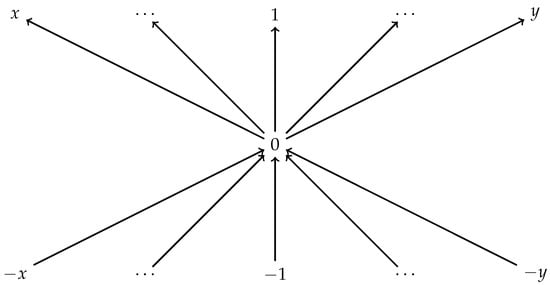
Figure 2. The directed graph associated to the strict partial order induced by the positive cone described in Example 15.

Indeed, in that case, one can demonstrate that if $a,b\in P$ are two distinct elements, then they are not comparable.

In the following example, we consider a more complex situation.

Example 18.

Consider the field of rational functions over the real numbers $\mathbb{R}\left(X\right)$. This field admits infinitely many positive cones. Below, we define a specific one, but our reasoning would apply to any of them. Every rational function $h\in \mathbb{R}\left(X\right)$ can be written uniquely in the following form:

$$h=x^k\frac{f}{g},\mathrm{where}f\left(0\right),g\left(0\right)\ne 0,k\in \mathbb{Z}.$$

We consider the positive cone $P:=\{h\in \mathbb{R}\left(X\right)\mid \frac{f\left(0\right)}{g\left(0\right)}>0\}$. We set $U:=\{h\in \mathbb{R}(X)\mid k=0\}$ and $\sum {\left(\mathbb{R}{\left(X\right)}^{\times }\right)}^2:=\{h\in \mathbb{R}\left(X\right)\mid h=h_1^2+\dots +h_n^{2}forsome{h}_1,\dots ,h_n\in \mathbb{R}{\left(X\right)}^{\times },n\in \mathbb{N}\}$. Consider the quotient hyperfield $F:=\mathbb{R}{\left(X\right)}_{E^{+}}$, where $E^{+}:=U\cap \sum {\left(\mathbb{R}{\left(X\right)}^{\times }\right)}^2$. In particular, $E^{+}\subseteq P$, since sums of non-zero squares are contained in any positive cones, and from Theorem 2 we obtain that F is real with the positive cone $P_{E^{+}}=\{{\left[h\right]}_{E^{+}}\mid h\in P\}$.

Take two elements $\left[h_1\right],\left[h_2\right]\in F$, such that

$$h_1=x^{k_1}\frac{f_1}{g_1},h_2=x^{k_2}\frac{f_2}{g_2}\mathrm{with}\frac{f_1\left(0\right)}{g_1\left(0\right)}>0,\frac{f_2\left(0\right)}{g_2\left(0\right)}>0.$$

First, assume that $k_1\ne k_2$. Without a loss of generality, let $k_1>k_2$. We compute

$$h_2-h{h}_1=x^{k_2}\frac{f_2{g}_{1}g-x^{k_1-k_2}{f}_1{g}_{2}f}{g_1{g}_{2}g},\mathrm{where}h=\frac{f}{g}\in E^{+}.$$

Then

$$\frac{(f_2{g}_{1}g-x^{k_1-k_2}{f}_1{g}_{2}f)\left(0\right)}{\left(g_1{g}_{2}g\right)\left(0\right)}=\frac{f_2\left(0\right)}{g_2\left(0\right)}>0.$$

Hence $\left[h_2\right]-\left[h_1\right]\subseteq P_{E^{+}}$, so $\left[h_2\right]>\left[h_1\right]$. Now assume that $k:=k_1=k_2$. We have

$$h_2-h{h}_1=x^k\frac{f_2{g}_{1}g-f_1{g}_{2}f}{g_1{g}_{2}g},\mathrm{where}h=\frac{f}{g}\in E^{+}.$$

Take $h=\frac{f}{g}$, such that $g\left(0\right)=1$ and $f\left(0\right)<\frac{\left(f_2{g}_1\right)\left(0\right)}{\left(f_1{g}_2\right)\left(0\right)}$. Then

$$\frac{(f_2{g}_{1}g-f_1{g}_{2}f)\left(0\right)}{\left(g_1{g}_{2}g\right)\left(0\right)}>0.$$

Hence, $(\left[h_2\right]-\left[h_1\right])\cap P_{E^{+}}\ne \varnothing$. On the other hand, let $g\left(0\right)=1$ and $f\left(0\right)>\frac{\left(f_2{g}_1\right)\left(0\right)}{\left(f_1{g}_2\right)\left(0\right)}$. Then

$$\frac{(f_2{g}_{1}g-f_1{g}_{2}f)\left(0\right)}{\left(g_1{g}_{2}g\right)\left(0\right)}<0.$$

Hence, $(\left[h_2\right]-\left[h_1\right])\cap -P_{E^{+}}\ne \varnothing$, so $(\left[h_1\right]-\left[h_2\right])\cap P_{E^{+}}\ne \varnothing$. This means that $\left[h_1\right]$ and $\left[h_2\right]$ are incomparable with respect to the partial order induced by $P_{E^{+}}$.

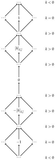
We illustrate in Figure 3 below the graph associated to the strict partial order induced by P on $\mathbb{R}\left(X\right)$.

Figure 3. The graph associated to the strict partial order induced by P on $\mathbb{R}\left(X\right)$.

The nodes situated above the central node labelled by 0 correspond to elements of P. The nodes below correspond to elements of $-P$. Each level of this graph, which is above the central node labelled by 0, corresponds to an integer k. For instance, the level of the node labelled by 1 consists of all the nodes situated on the left and on the right of the node labelled by 1 and corresponds to the integer $k=0$. The levels below this level correspond to positive integers $k>0$ and the levels above to negative integers $k<0$. Similarly, each level below the central node labelled by 0 correspond to an integer. There are no edges between any two nodes of the same level, as they are incomparable. If two nodes are in different levels, then they are connected in the upwards direction.

6. Further Research

In this paper, we have studied the notion of the positive cone in hyperfields. We have investigated the (directed) graph associated to the strict partial order induced by a positive cone in a hyperfield in some examples. What we have observed suggests a particular structure of this graph (that of a linear order and that of a star, as in Example 15, or a combination of these two, as in Example 18).

Moreover, we have considered the characteristic and the C-characteristic of hyperfields, and we have demonstrated how these interact to produce interesting results in the theory of hyperfields. In particular, we have obtained Theorem 6, which gives a criterion for deciding whether a given finite hyperfield cannot be obtained via Krasner’s quotient construction.

We have demonstrated that any positive integer larger than 1 can be realized as the characteristic of an infinite hyperfield (Theorem 3). We ask if it is possible to realize any characteristic with finite hyperfields as well. To try to answer this question, we have initially focused on the finite hyperfields of the form ${\left({\mathbb{F}}_p\right)}_G$ and developed an algorithm to compute their characteristic. At this point, we can provide the data in Table 1 below.

Table 1. Finite hyperfields of non-prime characteristic $\le 12$.

$char{\left({\mathbb{F}}_{\mathit{p}}\right)}_{\mathit{G}}$	p	G	$\left|\mathit{G}\right|$
4	29	$⟨16⟩$	7
6	199	$⟨125⟩$	11
8	2179	$⟨2118⟩$	11
9	2707	$⟨1085⟩$	11
10	7151	$⟨5825⟩$	11
12	62,323	⟨28,216⟩	13

The characteristic of a hyperfield of the form ${\left({\mathbb{F}}_p\right)}_G$ depends on p and on the multiplicative subgroup G of ${\mathbb{F}}_p^{\times }$. Since G is a cyclic group, we conclude that $char{\left({\mathbb{F}}_p\right)}_G$ depends on the prime number p and on the choice of a divisor d of $p-1$. This means that the number N of possible hyperfields increases very fast with p. For example, in the case of characteristic 12, before finding the hyperfield ${\left({\mathbb{F}}_{62323}\right)}_{⟨28216⟩}$, the algorithm would a priori have to generate and check the hyperfields corresponding to 6262 prime numbers, which gives a total of $N=$ 449,569 possibilities. Nevertheless, we can use Proposition 7 to substantially reduce the number of cases to be considered.

For example, if we are looking for a hyperfield of characteristic 12, then we would assume that $char{\left({\mathbb{F}}_p\right)}_G=12$, which by Proposition 7 cannot hold if $\left|G\right|$ is divisible by some prime number $<12$. Hence, we can restrict our attention to those prime numbers p, such that $p-1$ is divisible at least by one prime number $\ge 13$. Moreover, for these primes p, we can restrict our choice of the divisor of $p-1$ to those d, which are not divisible by primes $<12$. These restrictions reduce the number of hyperfields to be checked by the algorithm to 9871, which is approximately 2.19% of N.

Remark 10.

We know that $char{\left({\mathbb{F}}_p\right)}_G\ne 14$ for all prime numbers $p\le$ 160,000.

An analogous problem can be posed for the realization of C-characteristics, as Theorem 5 provides only infinite hyperfields. For the hyperfields of the form ${\left({\mathbb{F}}_p\right)}_G$, our algorithm provided the data in Table 2 below.

Table 2. Finite hyperfields of non-prime C-characteristic $\le 10$.

$C-char{\left({\mathbb{F}}_{\mathit{p}}\right)}_{\mathit{G}}$	p	G	$\left|\mathit{G}\right|$
4	151	$⟨59⟩$	5
6	953	$⟨879⟩$	7
8	15137	$⟨11803⟩$	11
9	26951	$⟨1202⟩$	11
10	44221	$⟨31076⟩$	11

Remark 11.

We know that $C-char{\left({\mathbb{F}}_p\right)}_G\ne 12$ for all prime numbers is $p\le 152897$.

Our algorithm does not consider hyperfields of the form ${\left({\mathbb{F}}_{p^k}\right)}_G$ with $k>1$.

Another natural question is if it is possible to somehow generalise Example 4 to construct finite real hyperfields of cardinality $>7$ with C-characteristic $>1$, thus providing further examples of non-quotient hyperfields.

References

- Krasner, M. Approximation des corps valués complets de caractéristique p ≠ 0 par ceux de caractéristique 0. In Colloque D’algèbre Supérieure, tenu à Bruxelles du 19 au 22 Décembre 1956; Centre Belge de Recherches Mathématiques, Établissements Ceuterick: Louvain, Belgium; Librairie Gauthier-Villars: Paris, France, 1957; pp. 129–206. [Google Scholar]
- Viro, O. Hyperfields for Tropical Geometry I. Hyperfields and dequantization. arXiv 2010, arXiv:1006.3034. [Google Scholar]
- Lee, J. Hyperfields, truncated DVRs, and valued fields. J. Number Theory 2020, 212, 40–71. [Google Scholar] [CrossRef]
- Connes, A.; Consani, C. From monoids to hyperstructures: In search of an absolute arithmetic. In Casimir Force, Casimir Operators and the Riemann Hypothesis; Walter de Gruyter: Berlin, Germany, 2010; pp. 147–198. [Google Scholar]
- Connes, A.; Consani, C. The hyperring of adèle classes. J. Number Theory 2011, 131, 159–194. [Google Scholar] [CrossRef]
- Marshall, M. Real reduced multirings and multifields. J. Pure Appl. Algebra 2006, 205, 452–468. [Google Scholar] [CrossRef]
- Lam, T.Y. Orderings, valuations and quadratic forms. In CBMS Regional Conference Series in Mathematics; American Mathematical Society: Providence, RI, USA, 1983; Volume 52, pp. vii+143. [Google Scholar] [CrossRef]
- Gładki, P.; Marshall, M. Orderings and signatures of higher level on multirings and hyperfields. J. K-Theory 2012, 10, 489–518. [Google Scholar] [CrossRef]
- Kuhlmann, K.; Linzi, A.; Stojałowska, H. Orderings and valuations in hyperfields. J. Algebra 2022, 611, 399–421. [Google Scholar] [CrossRef]
- Jun, J. Algebraic geometry over hyperrings. Adv. Math. 2018, 323, 142–192. [Google Scholar] [CrossRef]
- Krasner, M. A class of hyperrings and hyperfields. Internat. J. Math. Math. Sci. 1983, 6, 307–311. [Google Scholar] [CrossRef]
- Massouros, C.G. Methods of constructing hyperfields. Internat. J. Math. Math. Sci. 1985, 8, 725–728. [Google Scholar] [CrossRef]
- Marty, F. Sur une généralization de la notion de groupe. In Proceedings of the Huitiéme Congrès des Mathématiciens Scand, Stockholm, Sweden, 14–18 August 1934; pp. 45–49. [Google Scholar]
- Marty, F. Rôle de la notion de hypergroupe dans l’étude de groupes non abéliens. C. R. Acad. Sci. 1935, 201, 636–638. [Google Scholar]
- Marty, F. Sur les groupes et hypergroupes attaches à une fraction rationnelle. Ann. Sci. École Norm. Sup. 1936, 53, 83–123. [Google Scholar] [CrossRef]
- Massouros, C.; Massouros, G. An Overview of the Foundations of the Hypergroup Theory. Mathematics 2021, 9, 1014. [Google Scholar] [CrossRef]
- Linzi, A.; Cristea, I. Dependence Relations and Grade Fuzzy Set. Symmetry 2023, 15, 311. [Google Scholar] [CrossRef]
- Corsini, P.; Leoreanu, V. Applications of Hyperstructure Theory; Advances in Mathematics (Dordrecht); Kluwer Academic Publishers: Dordrecht, The Netherlands, 2003; Volume 5, pp. xii+322. [Google Scholar] [CrossRef]
- Tolliver, J. An equivalence between two approaches to limits of local fields. J. Number Theory 2016, 166, 473–492. [Google Scholar] [CrossRef]
- Mittas, J. Sur les hyperanneaux et les hypercorps. Math. Balkanica 1973, 3, 368–382. [Google Scholar]
- Massouros, C.G. On the theory of hyperrings and hyperfields. Algebra i Logika 1985, 24, 728–742, 749. [Google Scholar] [CrossRef]
- Baker, M.; Jin, T. On the structure of hyperfields obtained as quotients of fields. Proc. Am. Math. Soc. 2021, 149, 63–70. [Google Scholar] [CrossRef]
- Bergelson, V.; Shapiro, D.B. Multiplicative subgroups of finite index in a ring. Proc. Am. Math. Soc. 1992, 116, 885–896. [Google Scholar] [CrossRef]
- Turnwald, G. Multiplicative subgroups of finite index in a division ring. Proc. Am. Math. Soc. 1994, 120, 377–381. [Google Scholar] [CrossRef]
- Massouros, G.; Massouros, C. Hypercompositional Algebra, Computer Science and Geometry. Mathematics 2020, 8, 1338. [Google Scholar] [CrossRef]
- Ameri, R.; Eyvazi, M.; Hoskova-Mayerova, S. Advanced results in enumeration of hyperfields. AIMS Math. 2020, 5, 6552–6579. [Google Scholar] [CrossRef]
- Prestel, A.; Delzell, C.N. Mathematical Logic and Model Theory; A Brief Introduction, Expanded Translation of the 1986 German; Universitext; Springer: London, UK, 2011; pp. x+193. [Google Scholar] [CrossRef]
- Krasner, M. Sur la primitivité des corps P-adiques. Mathematika 1937, 13, 72–191. [Google Scholar]
- Engler, A.J.; Prestel, A. Valued Fields; Springer Monographs in Mathematics; Springer: Berlin, Germany, 2005; pp. x+205. [Google Scholar]
- Bowler, N.; Su, T. Classification of doubly distributive skew hyperfields and stringent hypergroups. J. Algebra 2021, 574, 669–698. [Google Scholar] [CrossRef]
Disclaimer/Publisher’s Note: The statements, opinions and data contained in all publications are solely those of the individual author(s) and contributor(s) and not of MDPI and/or the editor(s). MDPI and/or the editor(s) disclaim responsibility for any injury to people or property resulting from any ideas, methods, instructions or products referred to in the content. |
© 2023 by the authors. Licensee MDPI, Basel, Switzerland. This article is an open access article distributed under the terms and conditions of the Creative Commons Attribution (CC BY) license (https://creativecommons.org/licenses/by/4.0/).