Article

Optimal Model Averaging for Semiparametric Partially Linear Models with Censored Data

1
School of Mathematics and Statistics, Hefei Normal University, Hefei 230601, China
2
Faculty of Science, Beijing University of Technology, Beijing 100124, China
*
Author to whom correspondence should be addressed.
Mathematics 2023, 11(3), 734; https://doi.org/10.3390/math11030734
Submission received: 29 December 2022 / Revised: 25 January 2023 / Accepted: 28 January 2023 / Published: 1 February 2023
(This article belongs to the Special Issue Statistical Methods and Models for Survival Data Analysis)

Abstract

:
In the past few decades, model averaging has received extensive attention, and has been regarded as a feasible alternative to model selection. However, this work is mainly based on parametric model framework and complete dataset. This paper develops a frequentist model-averaging estimation for semiparametric partially linear models with censored responses. The nonparametric function is approximated by B-spline, and the weights in model-averaging estimator are picked up via minimizing a leave-one-out cross-validation criterion. The resulting model-averaging estimator is proved to be asymptotically optimal in the sense of achieving the lowest possible squared error. A simulation study demonstrates that the method in this paper is superior to traditional model-selection and model-averaging methods. Finally, as an illustration, the proposed procedure is further applied to analyze two real datasets.

1. Introduction

The semiparametric partially linear model (PLM), which was proposed by [1], has attracted extensive attention in statistics because it combines the interpretability of the linear model with the flexibility of the nonparametric model. A large collection of literature has explored the estimation methods of this model, including the parametric part and the nonparametric function, such as [2,3,4,5], and so on. The premise of using methods in the aforementioned literature is that the model is correctly specified. However, in real data analysis, researchers are always able to collect a variety of variables and are not sure which variables are to be included in the true model. This kind of uncertainty is generally referred to as model uncertainty, which brings great trouble to statistical analysis.
Refs. [6,7,8] pointed out that model selection and model averaging are two mainstream methods to deal with model uncertainty. Model selection, which has a long history, selects a model from a series of candidate models through selection criteria, for example, Akaike information criterion (AIC [9]), Bayesian information criterion (BIC [10]), focused information criterion (FIC [11]), and so on. In addition, shrinkage-estimation-based variable selection was also applied to determine which variables are neededto build a PLM (see, e.g., [12,13,14], among others). These model-selection methods can be viewed as combining a series of candidate models, and assigning a weight of 1 to the selected model and 0 to other models.
As an important alternative to model selection, model averaging incorporates the model uncertainty in statistical analysis by assigning nonzero weight vector to a set of candidate models, which frequently leads to more effective results (see [15]). Bayesian model averaging, which is an important branch of model averaging, has been fully developed in the past decades; see [16] for details. In the current paper, we focus on model-averaging approach in PLM from a frequentist perspective. Since ref. [17] pioneered the use of Mallows criterion for weight choice in model averaging, there is rapidly growing research on asymptotically optimal model averaging. Different kinds of optimal model-averaging methods were proposed, including jackknife model averaging (JMA [7]), Kullback–Leibler model averaging [18], generalized least-squares model averaging [19], leave-subject-out cross-validation [20], K-fold cross-validation [21], and so on. In addition, the optimal model-averaging methods were extended to quantile regression [22], semiparametric models [23,24], missing data [25,26], functional data [27], measurement error data [28], and high-dimensional data [29,30].
Censored data are ubiquitous in the fields of biomedicine, industry, econometrics, etc. For example, in biomedicine, when some sampled individuals are lost to follow-up before the end of the study or drop out during the study, the survival time will be subject to censoring. Compared with the complete data, censoring makes some data unable to be observed completely, which increases the difficulty of statistical analysis. Although an extensive body of literature focusing on the estimation methods in the presence of censored data has been developed, such as [31,32], there is little work on the development of model-averaging approaches with censored data. Based on FIC advocated in [11,33,34,35], theydeveloped model-averaging methods for different regression models with censored data under the local misspecification framework, where the weights of the model-averaging estimators were constructed by the information criterion values, rather than being selected in a data-driven fashion. Moreover, the framework mentioned above requires that the distance between the candidate model and the true model is O   ( 1 / n ) . This means the candidate model is close to the true model when the sample size is large, which is unrealistic.
Without local misspecification framework, ref. [36] constructed the optimal model-averaging estimator for a high-dimensional linear model with censored data by adapting a leave-one-out cross-validation criterion. Ref. [37] studied Mallows model-averaging method for linear models with censored responses, and the resulting model-averaging estimator was proved to be asymptotically optimal in terms of minimizing the squared error loss. The optimal model-averaging methods for censored data mentioned above are based on classical linear models. The primary object of the current paper is to construct an optimal model-averaging estimator for semiparametric PLM with censored responses, in which the weight vector is selected by minimizing a leave-one-out cross-validation criterion. Compared with [36,37], we confront two major challenges. Firstly, the nonparametric function in PLM significantly complicates the construction of the model-averaging estimator and the development of the weight choice criterion. Secondly, our proof of optimality cannot follow the approach of the linear model, since their proof techniques cannot be directly applied when a nonparametric part is present.
The plan of this article is as follows. In Section 2, we describe the model set and introduce the parametric estimation method in the candidate PLM. Section 3 constructs the model-averaging estimator and proposes a weight choice criterion. Section 4 establishes the asymptotic optimality of the model-averaging estimator. Section 5 explores the finite sample performance of our method by the simulation study. Section 6 applies the proposed method to a real dataset. Section 7 gives some conclusions. Proofs are listed in the Appendix A.

2. Model Setup and Parametric Estimation

To facilitate presentation, we first list the basic notations used in this paper in Table 1. Then, we consider the following PLM:
Y i = μ i + ϵ i = j = 1 x i j β j + g ( U i ) + ϵ i , i = 1 , , n ,
where Y i is a response variable with a continuous distribution function F ( · ) , a countably infinite vector X i = ( x i 1 , x i 2 , ) is linearly related to Y i , U i is a covariate nonlinearly related to Y i , g ( · ) is an unknown smooth function, and ϵ i is the model error with E ( ϵ i | X i , U i ) = 0 and E ( ϵ i 2 | X i , U i ) = σ i 2 . The covariate U i is distributed on a compact interval [ a , b ] . Without loss of generality, we take [ a , b ] = [ 0 , 1 ] . The conditional expectation of the response is denoted as E ( Y i | X i , U i ) = μ i = j = 1 x i j β j + g ( U i ) .
In survival analysis, we assume Y i to be a known monotonic transformation of the survival time T i , for example, the commonly used logarithm Y i = log T i . Y i may be censored by a censoring time C i and hence cannot be observed completely. We consider a sample of independent observations ( Z i , δ i , X i , U i ) for i = 1 , , n , where Z i = min ( Y i , C i ) and δ i = I ( Y i C i ) is the censoring indicator.
Let G ( · ) be the cumulative distribution function of the censoring time, and Z G , i = Z i δ i / { 1 G ( Z i ) } be a synthetic response. Then, from [38], it is not difficult to verify that E ( Z G , i | X i , U i ) = E ( Y i | X i , U i ) = μ i . Therefore, under model (1), we obtain
Z G , i = μ i + e G , i = j = 1 x i j β j + g ( U i ) + e G , i , i = 1 , , n ,
where E ( e G , i | X i , U i ) = 0 and E ( e G , i 2 | X i , U i ) = σ G , i 2 . Model (2) can be expressed in matrix form as
Z G = μ + e G = X β + M + e G ,
where Z G = ( Z G , 1 , , Z G , n ) is an n-dimensional synthetic response vector, conditional mean μ = ( μ 1 , , μ n ) is an n-dimensional vector, M = { g ( U 1 ) , , g ( U n ) } , X = ( X 1 , , X n ) is a linear covariate matrix, U = ( U 1 , , U n ) , and e G = ( e G , 1 , , e G , n ) is an n-dimensional error vector satisfying E ( e G | X , U ) = 0 and E ( e G e G | X , U ) = Ω G = diag ( σ G , 1 2 , , σ G , n 2 ) .
Assume that we have a total of S candidate PLMs to approximate the true data generating process, where S is allowed to go to infinity. Suppose the sth candidate model is
Z G = μ ( s ) + e G , ( s ) = X ( s ) β ( s ) + M ( s ) + e G , ( s ) ,
where X ( s ) = ( X ( s ) , 1 , , X ( s ) , n ) is an n × p s covariate matrix which includes p s columns of X with full column rank, β ( s ) = ( β ( s ) 1 , , β ( s ) p s ) is the corresponding p s × 1 unknown linear regression coefficient vector, M ( s ) = { g ( s ) ( U 1 ) , , g ( s ) ( U n ) } is an n × 1 unknown nonparametric function vector, and e G , ( s ) is the model error.
To obtain the estimator of μ under the sth candidate model, we should estimate the coefficient vector β ( s ) and nonparametric function vector M ( s ) firstly. There are many estimation methods for model (4), including kernel smoothing, polynomial spline smoothing, and so on. Recently, ref. [39] pointed out that using B-splines to approximate nonparametric functions in the area of model averaging has great advantages; therefore, in this paper, we adopt the spline technique to estimate the unknowns in model (4).
Denote ψ n = { 0 = u 0 < u 1 < < u J n < u J n + 1 = 1 } as a partition of [ 0 , 1 ] , where J n is the number of interior knots. Let ζ n be the polynomial spline space on interval [ 0 , 1 ] of degree r. From [40], the nonparametric function in PLM can be well estimated by a B-spline expansion. Then, for g s ( u ) , one can write
g ( s ) ( u ) B ( s ) ( u ) α ( s ) ,
where B ( s ) ( · ) = ( B ( s ) 1 ( · ) , , B ( s ) k n ( · ) ) is the normalized B-spline basis function vector in the sth candidate model, k n = J n + r + 1 , and α ( s ) = ( α ( s ) 1 , , α ( s ) k n ) is the vector of spline coefficient. Define the n × k n matrix B ( s ) = ( B ( s ) ( U 1 ) , , B ( s ) ( U n ) ) . Therefore, there exists a design matrix X ( s ) * = ( X ( s ) , B ( s ) ) and the corresponding unknown parameter vector γ = ( β , α ) such that
μ ( s ) X ( s ) * γ ,
where X ( s ) * is supposed to be of full-column rank. By regressing Z G on X ( s ) * , we can obtain the least-squares estimators of β ( s ) and α ( s ) :
β ^ G , ( s ) = { X ( s ) ( I Q ( s ) ) X ( s ) } 1 X ( s ) ( I Q ( s ) ) Z G ,
and
α ^ G , ( s ) = ( B ( s ) B ( s ) ) 1 B ( s ) ( Z G X ( s ) β ^ ( s ) ) ,
where Q ( s ) = B ( s ) ( B ( s ) B ( s ) ) 1 B ( s ) . Therefore, the estimator of μ under the sth candidate model is given by
μ ^ G , ( s ) = X ( s ) β ^ G , ( s ) + B ( s ) α ^ G , ( s ) = { Q ( s ) + X ˜ ( s ) ( X ˜ ( s ) X ˜ ( s ) ) 1 X ˜ ( s ) } Z G = P ( s ) Z G ,
where X ˜ ( s ) = ( I Q ( s ) ) X ( s ) , and P ( s ) = Q ( s ) + X ˜ ( s ) ( X ˜ ( s ) X ˜ ( s ) ) 1 X ˜ ( s ) . From Equation (9), we find that μ ^ G , ( s ) is linearly dependent on Z G .

3. Model-Averaging Estimator and Weight Choice Criterion

Let ω = ( ω 1 , , ω S ) be a weight vector belonging to the set W = { ω [ 0 , 1 ] S : s = 1 S ω s = 1 } , then the model-averaging estimator of μ can be formulated as
μ ^ G ( ω ) = s = 1 S ω s μ ^ G , ( s ) = P ( ω ) Z G ,
where P ( ω ) = s = 1 S ω s P ( s ) .
Motivated by [7], we propose a leave-one-out cross-validation criterion to select the weight vector ω for Equation (10) in the PLM framework. Let X ( s ) [ i ] , B ( s ) [ i ] and Z G [ i ] be the matrices/vectors X ( s ) , B ( s ) and Z G with the ith row deleted. The leave-one-out estimator of μ i in the sth candidate model is given by
μ ˜ G , ( s ) , i = X ( s ) , i β ^ G , ( s ) [ i ] + B ( s ) ( U i ) α ^ G , ( s ) [ i ] ,
where
β ^ G , ( s ) [ i ] = X ( s ) [ i ] ( I Q ˜ ( s ) ) X ( s ) [ i ] 1 X ( s ) [ i ] ( I Q ˜ ( s ) ) Z G [ i ] ,
α ^ G , ( s ) [ i ] = B ( s ) [ i ] B ( s ) [ i ] 1 B ( s ) [ i ] Z G [ i ] X ( s ) [ i ] β ^ G , ( s ) [ i ] ,
and Q ˜ ( s ) = B ( s ) [ i ] ( B ( s ) [ i ] B ( s ) [ i ] ) 1 B ( s ) [ i ] . Denote the sth jackknife estimator and the corresponding jackknife version of the averaging estimator as μ ˜ G , ( s ) = ( μ ˜ G , ( s ) , 1 , , μ ˜ G , ( s ) , n ) and μ ˜ G ( ω ) = s = 1 S ω s μ ˜ G , ( s ) . The leave-one-out cross-validation weight choice criterion is
C V G ( ω ) = Z G μ ˜ G ( ω ) 2 ,
then minimizing C V G ( ω ) over the space W yields the optimal weight vector. However, in practice, such a minimization process is computationally infeasible because the cumulative distribution function G ( · ) in Equation (12) is unknown and needs to be estimated. Similar to [41], we can estimate G ( · ) by the commonly used Kaplan–Meier estimator
G ^ n ( z ) = 1 i = 1 n n i n i + 1 I [ Z ( i ) z , δ ( i ) = 0 ] ,
where Z ( 1 ) Z ( 2 ) Z ( n ) denote the order statistics of Z 1 , Z 2 , , Z n , and δ ( i ) is the indicator corresponding to Z ( i ) . In what follows, a letter subscripted by G ^ n denotes that it is obtained by replacing G in its corresponding estimator with G ^ n . For instance, Z G ^ n is obtained by replacing G with its estimator G ^ n in Z G . Then a feasible counterpart of C V G ( ω ) is given by
C V G ^ n ( ω ) = Z G ^ n μ ˜ G ^ n ( ω ) 2 ,
where μ ˜ G ^ n ( ω ) = s = 1 S ω s μ ˜ G ^ n , ( s ) , and μ ˜ G ^ n , ( s ) = ( μ ˜ G ^ n , ( s ) , 1 , , μ ˜ G ^ n , ( s ) , n ) . Minimizing C V G ^ n ( ω ) with respect to ω over the set W leads to the jackknife choice of weight vector
ω ^ = arg min ω W C V G ^ n ( ω ) .
Plugging G ^ n and ω ^ into Equation (10) yields the model-averaging estimator of μ , written as μ ^ G ^ n ( ω ^ ) , which is named the censored partially linear model averaging (CPLMA) estimator hereafter.
However, minimizing the weight choice criterion (14) is not easy because the computation of μ ˜ G ^ n , ( s ) requires n separate regressions, which is especially cumbersome when the number of candidate models and the sample sizes are large. Motivated by the computationally efficient cross-validation criterion introduced by [7] for linear regression model, we express μ ˜ G ^ n , ( s ) in a simple form which yields an enormous reduction in calculation time. Let ϕ i i ( s ) be the ith diagonal entry of P ( s ) . From [20,42], μ ˜ G ^ n , ( s ) can be conveniently written as
μ ˜ G ^ n , ( s ) = { P ( s ) D ( s ) A ( s ) } Z G ^ n = P ˜ ( s ) Z G ^ n ,
where D ( s ) = diag ( D 11 ( s ) , , D n n ( s ) ) , D i i ( s ) = ϕ i i ( s ) + ( ϕ i i ( s ) ) 2 + ( ϕ i i ( s ) ) 3 + = ϕ i i ( s ) / ( 1 ϕ i i ( s ) ) , and A ( s ) = I P ( s ) . The shortcut formula of μ ˜ G ^ n , ( s ) given in (16) indicates that all elements in μ ˜ G ^ n , ( s ) can be simultaneously calculated based on all observations, which is much more convenient and time-saving than the standard method based on Equation (11). Let Λ ( s ) = D ( s ) A ( s ) , Λ ( ω ) = s = 1 S ω s Λ ( s ) , and A ( ω ) = s = 1 S ω s A ( s ) = I P ( ω ) . The corresponding computational shortcut formula for the feasible jackknife criterion (14) then follows as
C V G ^ n ( ω ) = Z G ^ n { P ( ω ) Λ ( ω ) } Z G ^ n 2 = { A ( ω ) + Λ ( ω ) } Z G ^ n 2 = Z G ^ n { A ( ω ) + Λ ( ω ) } { A ( ω ) + Λ ( ω ) } Z G ^ n = ω H G ^ n H G ^ n ω ,
where H G ^ n = { ( A ( 1 ) + Λ ( 1 ) ) Z G ^ n , , ( A ( S ) + Λ ( S ) ) Z G ^ n } is an n × S matrix. From Equation (17), we observe that the minimization of C V G ^ n ( ω ) is a standard quadratic programming problem, which can be performed by various existing software packages, for example, the quadprog package in R [43].

4. Asymptotic Optimality

In this section, we demonstrate that the resulting weight vector, which is obtained by minimizing the weight choice criterion C V G ^ n ( ω ) , is asymptotically optimal under some mild conditions.
Define the squared loss as L G ( ω ) = μ ^ G ( ω ) μ 2 , and the corresponding risk function as R G ( ω ) = E ( L G ( ω ) | X , U ) = A ( ω ) μ 2 + tr { P ( ω ) Ω G P ( ω ) } . Let p ¯ = max 1 s S p s , q ¯ = max 1 s S rank ( B ( s ) ) , ξ G = inf ω W R G ( ω ) , and ω s 0 be a S × 1 vector with the sth entry taking on 1 and the others taking on 0. To prove the asymptotic optimality of the model-averaging estimator μ ^ G ^ n ( ω ^ ) , we list the following regularity conditions, where all limiting processes correspond to n .
  • (Condition (C.1)) τ F < τ G , where τ L = inf { t : L ( t ) = 1 } for any distribution function L.
  • (Condition (C.2)) λ ¯ ( Ω G ) C G , where λ ¯ ( · ) denotes the maximum singular value of a matrix, and C G is a constant.
  • (Condition (C.3)) ξ G 2 s = 1 S R G ( ω s 0 ) 0 , a.s.
  • (Condition (C.4)) p ¯ ξ G 1 0 and q ¯ ξ G 1 0 , a.s.
  • (Condition (C.5)) μ 2 = O ( n ) , a.s.
  • (Condition (C.6)) ϕ i i ( s ) C s n 1 tr ( P ( s ) ) , a.s., where C s is a constant.
  • (Condition (C.7)) The function g belongs to a class of functions A , whose rth derivative g ( r ) exsits and is Lipschitz of order α 0 . That is,
    A = { g ( · ) : | g ( r ) ( t 1 ) g ( r ) ( t 0 ) | M | t 1 t 0 | α 0 f o r t 1 , t 0 U } ,
    for some positive constant M , where U is the support of U, r is a nonnegative integer and α 0 ( 0 , 1 ] such that r + α 0 > 0.5 .
Condition (C.1), which is the same as condition (C5) in [35], is widely used to ensure the uniform convergence of the Kaplan–Meier estimator G ^ n ( · ) in studies of the censored data. Condition (C.2) imposes a mild restriction on the maximum singular value of the covariance matrix Ω G , which is also used by [44]. Condition (C.3), which is from condition (21) of [45], is less restrictive than the commonly used condition S ξ G 2 N s = 1 S { R G ( ω s 0 ) } N 0 , a . s . , for some constant N 1 in model-averaging references. Condition (C.4) places constraints on the growth rates of p ¯ and q ¯ , which is similar to condition (22) in [45]. Condition (C.5) discusses the sum of μ i 2 , and is frequently used in the model-averaging literature, such as [23,24], and so on. Condition (C.6) is a common assumption utilized to guarantee the asymptotic optimality of cross-validation; see [7,24], for instance. Conditions (C.3)–(C.6) require almost sure convergence, which ensure that the result (18) holds whether the covariates X and U are random or not. Specifically, when X and U are nonstochastic, we only need to assume convergence in probability in conditions (C.3)–(C.6); see [46]. Otherwise, we should impose almost sure convergence to guarantee that the proof method, which is used in the case of nonstochastic, is still effective. Condition (C.7) is required for the B-spline approximation in PLM; see [39,47].
Theorem 1 indicates that the CPLMA estimator proposed in this paper is asymptotically optimal in the sense that its squared error loss is asymptotically equivalent to that of the infeasible best possible model-averaging estimator in PLM framework. The proof of Theorem 1 is shown in the Appendix A.
Theorem 1.
Under Conditions (C.1)–(C.7), we have
L G ^ n ( ω ^ ) inf ω W L G ^ n ( ω ) 1
in probability as n .

5. A Simulation Study

In this section, a simulation experiment is conducted to investigate the finite sample performance of the CPLMA estimator, which arises from the proposed leave-one-out cross-validation weight choice approach, in PLM with censored responses. We compare it with several popular information-criterion-based model-selection methods as well as other model-averaging procedures.

5.1. The Design of Simulation

The data-generating process in this part is similar to the infinite-order regression model proposed by [17], except that responses are subject to censoring and a nonparametric function is included in addition to the linear part. Specifically, the data are generated by the following regression model:
Y i = μ i + ϵ i = j = 1 200 x i j β j + g ( U i ) + ϵ i ,
where X i = ( x i 1 , , x i 200 ) , the covariates in linear component, follows a multivariate normal distribution with mean 0 and covariance 0.5 j 1 j 2 between x i j 1 and x i j 2 . The coefficients of the linear part are set as β j = 1 / j α , and the parameter α varies between 2 and 0.5 . The larger α implies that the coefficient decays more quickly as j increases. The nonparametric function is g ( U i ) = sin ( 2 π U i 2 ) , where U i is generated from the uniform distribution on [ 0 , 1 ] . The model error ϵ i follows a normal distribution N ( 0 , η 2 ( x i 2 2 + 0.01 ) ) . We choose the value of η so that R 2 = v a r ( μ i ) / v a r ( Y i ) varies from 0.1 to 0.9 , where v a r ( · ) denotes the sample variance. In addition, the censoring variable C i is generated from a uniform distribution on interval [ a 1 , a 2 ] , where different values of a 1 and a 2 are selected to yield a censoring rate (CR) of either 20 % or 40 % . In order to evaluate the performance of the methods as comprehensively as possible, we consider two designs and set the sample size n = 50 , 75, 100, 200, 300, and 400.
Design 1
(non-nested setting).The linear parts of all candidate models are a subset of { x i 1 , , x i 5 } (with the rest of X i being ignored), so the number of candidate models is 2 5 = 32 .
Design 2
(nested setting).The sth candidate model includes the first s linear variables. The number of the candidate models is determined by S = INT ( 3 n 1 / 3 ) , where INT ( b ) denotes the nearest integer of b. Therefore, S = 11 , 13, 14, 18, 20, and 22, for n = 50 , 75, 100, 200, 300, and 400, respectively.

5.2. Estimation and Comparison

Suggested by [35], the cubic B-spline is used to approximate the nonparametric function, and the spline basis matrix is generated by b s ( · ) in splines package with R project [48]. To select the number of knots, we set η = 1 , α = 2 , and investigate the impact of the number of knots on the risk of CPLMA estimator under different scenarios. Figure 1 shows the variation for the mean of risks when the number of knots varies, over 500 replications for four combinations of designs and CRs considered. From Figure 1, we see that in almost all cases, 1 knot yields the smallest mean of risk, except that in the left lower panel, 1 knot leads to a mean of risk that is second to 2 knots but best among the remaining number of knots. In addition, in all cases, the mean of risk increases with the number of knots when the number of knots exceeds 2. This observation coincides with the findings in [39] that the larger number of knots results in a more serious overfitting effect. Therefore, the number of knots is set to be 1 in the simulation studies.
We compare the performance of the CPLMA method with two traditional model-selection methods (AIC and BIC) and two model-averaging methods based on scores of information criteria (SAIC and SBIC). For the sth model, we calculate AIC and BIC scores by
A I C s = log ( σ ^ G ^ n , ( s ) 2 ) + 2 n 1 t r ( P ( s ) ) ,
and
B I C s = log ( σ ^ G ^ n , ( s ) 2 ) + n 1 t r ( P ( s ) ) log ( n ) ,
respectively, where σ ^ G ^ n , ( s ) 2 = n 1 Z G ^ n μ ^ G ^ n , ( s ) 2 , and μ ^ G ^ n , ( s ) is obtained by replacing G in Equation (9) with G ^ n . Both methods pick the model with the smallest information criterion score.
For SAIC and SBIC, the weights of sth model are defined as
ω A I C s = exp ( A I C s / 2 ) / s = 1 S exp ( A I C s / 2 ) ,
and
ω B I C s = exp ( B I C s / 2 ) / s = 1 S exp ( B I C s / 2 ) ,
respectively. To evaluate these five methods, we draw 500 independent samples of size n, and compute the risk of the estimator of μ . For comparison convenience, the risks of all estimators are normalized by the risk produced by the AIC method.

5.3. Results

The simulation results for Design 1 are presented in Figure 2 and Figure 3 for the censoring rate of 20 % and in Figure 4 and Figure 5 for the censoring rate of 40 % . These four figures show that our method CPLMA leads to the smallest risk in most cases, except that both SAIC and SBIC sometimes have marginal advantages over ours when R 2 is large, and the advantage of SBIC is more obvious when n is small. In particular, comparing the simulation results between α = 0.5 and α = 2 , we find that the performance of CPLMA is better when α is small. As expected, SAIC and SBIC invariably produce vastly more accurate outcomes than their respective model-selection counterparts.
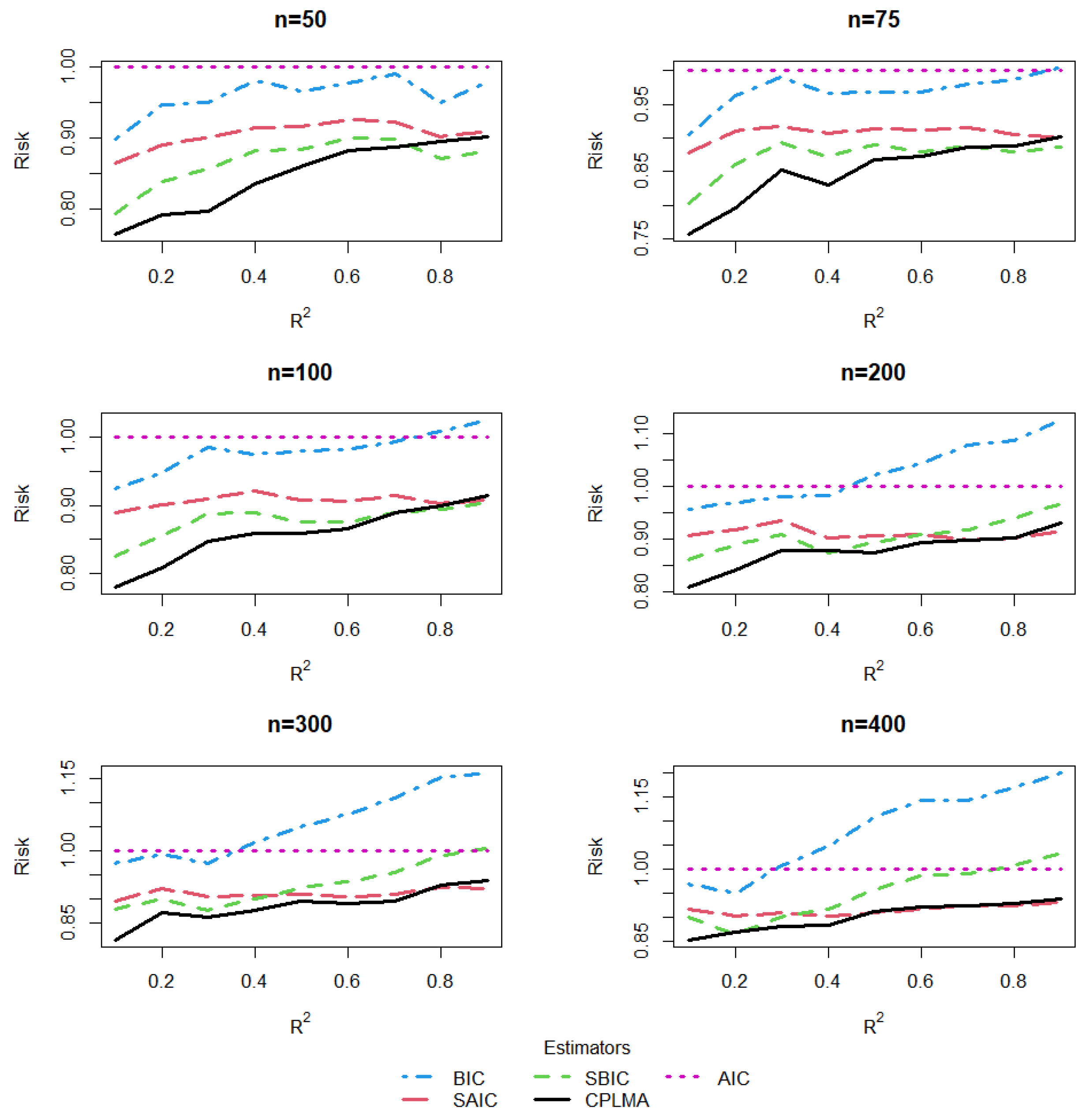
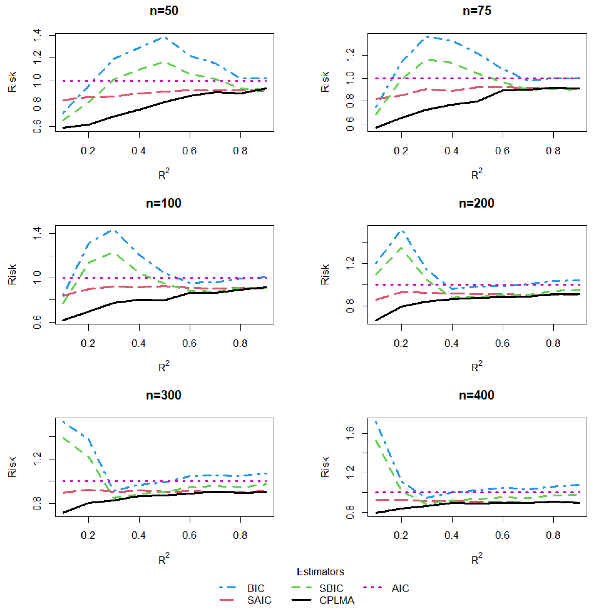
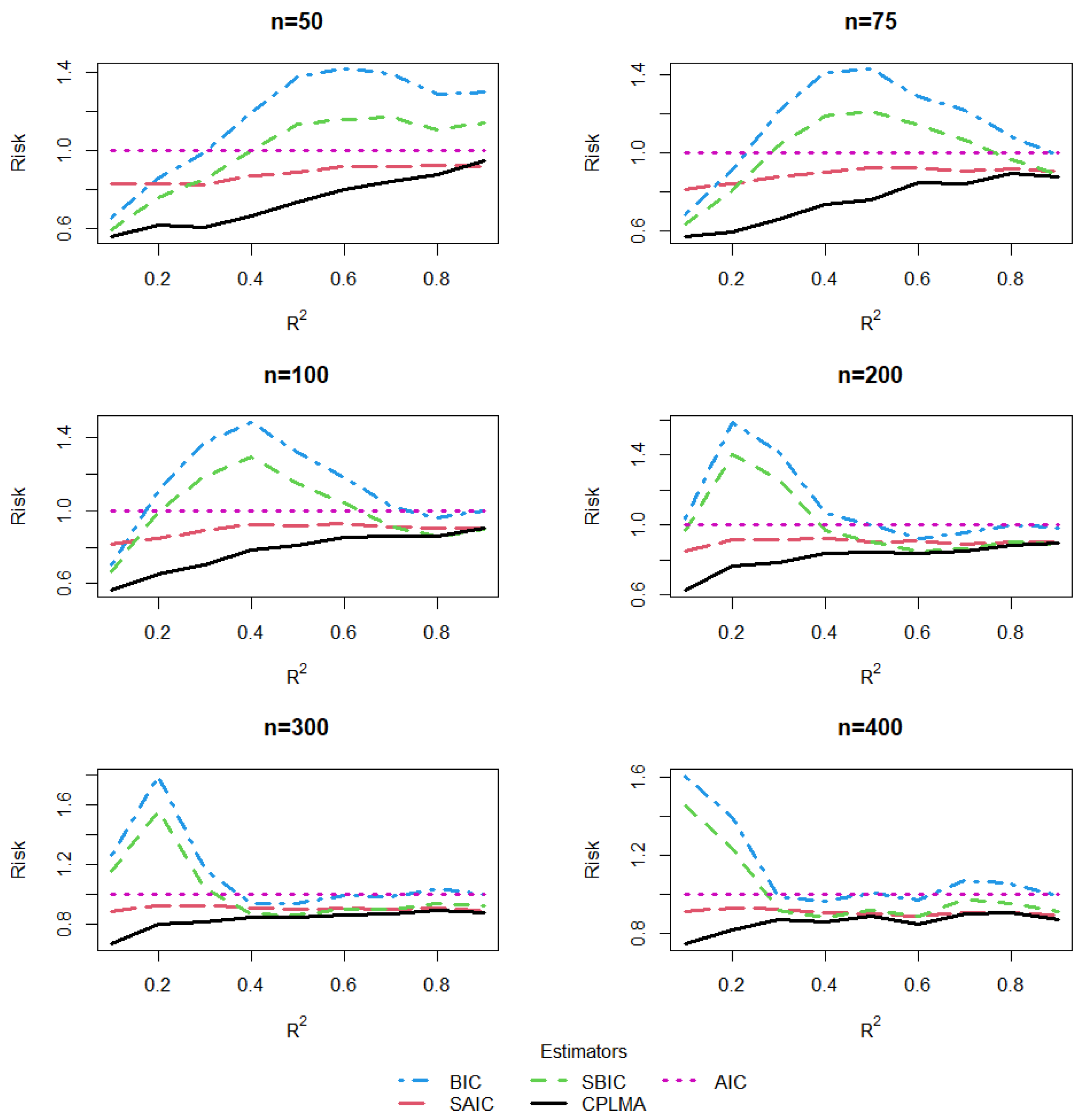
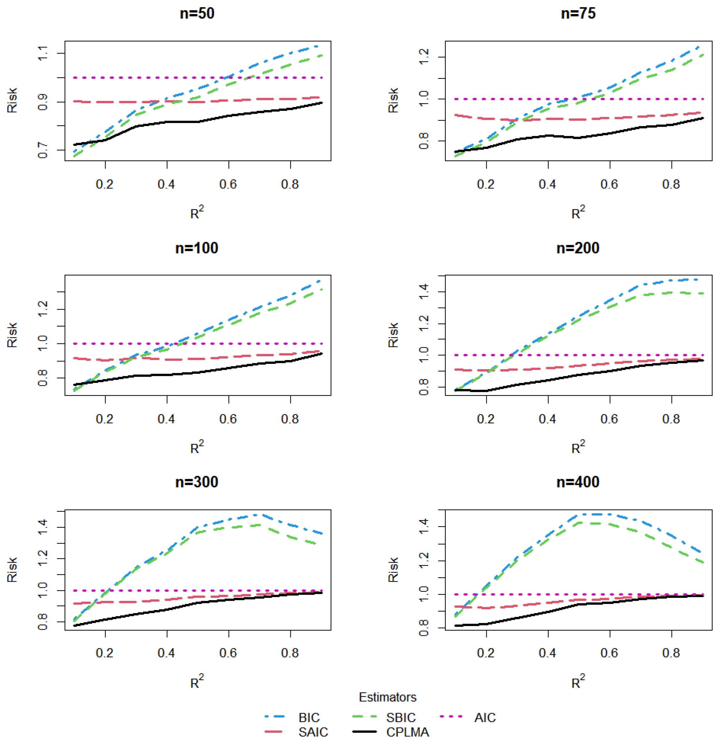
The simulation results for Design 2 are depicted in Figure 6, Figure 7, Figure 8 and Figure 9 with C R 20 % and 40 % , from which we see that in most cases our proposed CPLMA method still outperforms its rivals in terms of risk. The superiority of the CPLMA method over the other methods is more apparent than in Design 1. Additionally, we find that BIC-based model selection and averaging estimators have much worse risk performance than the other three estimators when R 2 is small, which is different from the simulation results in Design 1. We also note that SAIC and our method CPLMA almost perform equally well when R 2 is very large.
In a word, no matter whether the candidate models are nested or not, our proposal, CPLMA, is superior to the traditional model-selection and model-averaging methods for all the combinations of censoring rates and sample sizes considered.

6. Real Data Analysis

In this section, we apply the proposed CPLMA method to analyze two real datasets by R software. The first real dataset can be found in the R package “survival” [49], and the other is available at http://llmpp.nih.gov/MCL (accessed on 18 January 2023).

6.1. Primary Biliary Cirrhosis Dataset Study

The primary biliary cirrhosis (PBC) dataset includes information of 424 patients, which were collected at Mayo Clinic from January 1974 to May 1984, and has been extensively explored by [34,35,37,50,51]. Following the related literature, we restrict our attention to the n = 276 patients without missing observations, each of whom contains the data of 17 covariates. There are 111 deaths among 276 patients, which leads to 60 % of censoring.
In this dataset, the dependent variable is the log number of days between registration and the earlier of death or study analysis time in 1986. The 17 covariates include age (in years), albumin (serum albumin in g/dL), alk.phos (alkaline phosphotase in U/L), bili (serum bilirunbin in mg/dL), chol (serum cholesterol in mg/dL), copper (urine copper in ug/day), platelet (platelet count), protime (standardized blood clotting time in seconds), ast (aspartate aminotransferase, once called SGOT in U/mL), trig (triglycerides in mg/dL), ascites (presence of ascites, 0 = no, 1 = yes), edema ( 0 = no; 0.5 = yes, but responded to diuretic treatment; 1 = yes, did not respond to treatment), hepato (presence of hepatomegaly, 0 = no, 1 = yes), sex ( 0 = male, 1 = female), spiders (presence of spiders, 0 = no, 1 = yes), stage (histologic state of disease, graded 1, 2, 3, or 4), and trt (treatment code, 1 = D-pencillamine, 2 = placebo). The first 10 variables are continuous, which are standardized to have mean of 0 and variance of 1 in the analysis.
A total of 17 covariates lead to a huge number of candidate models, which brings heavy calculation burden. Ref. [50] pointed out that only eight covariates, that is, ge, edema, bili, albumin, copper, ast, protime, and stage, have significant impact on the response variable, and ref. [35] found that albumin has a functional impact on the response variable. Thus, we only consider eight significant covariates. Specifically, we assign albumin in the nonparametric part while including others in the linear part of PLM, and we run model selection and averaging on the covariates in the linear part. Accordingly, there are 2 7 = 128 prepared models as candidates. Similar to [35], we also use the cubic B-spline with two knots to approximate the nonparametric component.
To evaluate the prediction effect of two model-selection methods (AIC and BIC) and three model-averaging methods (SAIC, SBIC, and CPLMA), we randomly separate the data into a training sample and a test sample. Let n 0 be the size of the training sample, and n 1 = n n 0 be the size of the test sample. We set n 0 to 140 , 160 , 180 , 200 , 220 , and 240. The mean-squared prediction error (MSPE) is used to describe the out-of-sample prediction performance of the proposed CPLMA and its competitors. We further calculate the mean and the median of the MSPE for each method based on 1000 replications. Specifically,
MSPE mean = 1 1000 d = 1 1000 MSPE ( d ) ,
and
MSPE median = median d = 1 , 2 , , 1000 MSPE ( d ) ,
where
MSPE ( d ) = 1 n 1 i = n 0 + 1 n ( Z G ^ n , i ( d ) μ ^ i ( d ) ) 2 ,
and μ ^ i ( d ) is the predicted value of μ i in the dth repetition.
To facilitate comparison, we calculate the ratio of MSPE for a given method to the MSPE produced by AIC, which is referred to relative MSPE (RMSPE). Table 2 reports the mean and median of RMSPE across 1000 repetitions. We see that our proposed CPLMA always yields the lowest mean and median of RMSPE for all considered training sample sizes. In all cases, the values of RMSPE for BIC are bigger than 1 and the values of RMSPE for three model-averaging methods are smaller than 1, which indicates that in terms of prediction performance, AIC is the overwhelming favorite of two model-selection methods, and model-averaging methods outperform model-selection methods.
Table 3 presents the Diebold and Mariano (DM) [52] test results for the differences in MSPE, where a positive DM statistic implies that the method in the numerator yields a larger MSPE than the method in the denominator. The results in columns 6, 9, 11, and 12 indicate that the differences between CPLMA and its competitors are statistically significant, and our method always produces smaller MSPE than other four methods, which again demonstrates the superiority of our proposal. The results in column 3 show that AIC is significantly better than BIC, which coincides with the finding in Table 2. Columns 4 and 8 indicate that SAIC and SBIC are significantly different from their respective model-selection counterparts.

6.2. Mantle Cell Lymphoma Data Analysis

The mantle cell lymphoma (MCL) dataset contains 92 patients who were classified as having MCL based on established morphologic and immunophenotype criteria. Since 2003, this dataset has been widely studied by [53,54]. The response variable of interest is time (time of follow-up in year). The variable status denotes patient status at follow-up ( 1 = death, 0 = censored). The six covariates include indicator of INK/ARF deletion ( 1 = yes, 0 = no), indicator of ATM deletion ( 1 = yes, 0 = no), indicator of P-53 deletion ( 1 = yes, 0 = no), cyclinD-1 taqman result, BMI expression, and proliferation signature averages. After removing seven records with missing covariates, we focus on the information of the remaining 85 patients, and the censoring rate is 29.41 % .
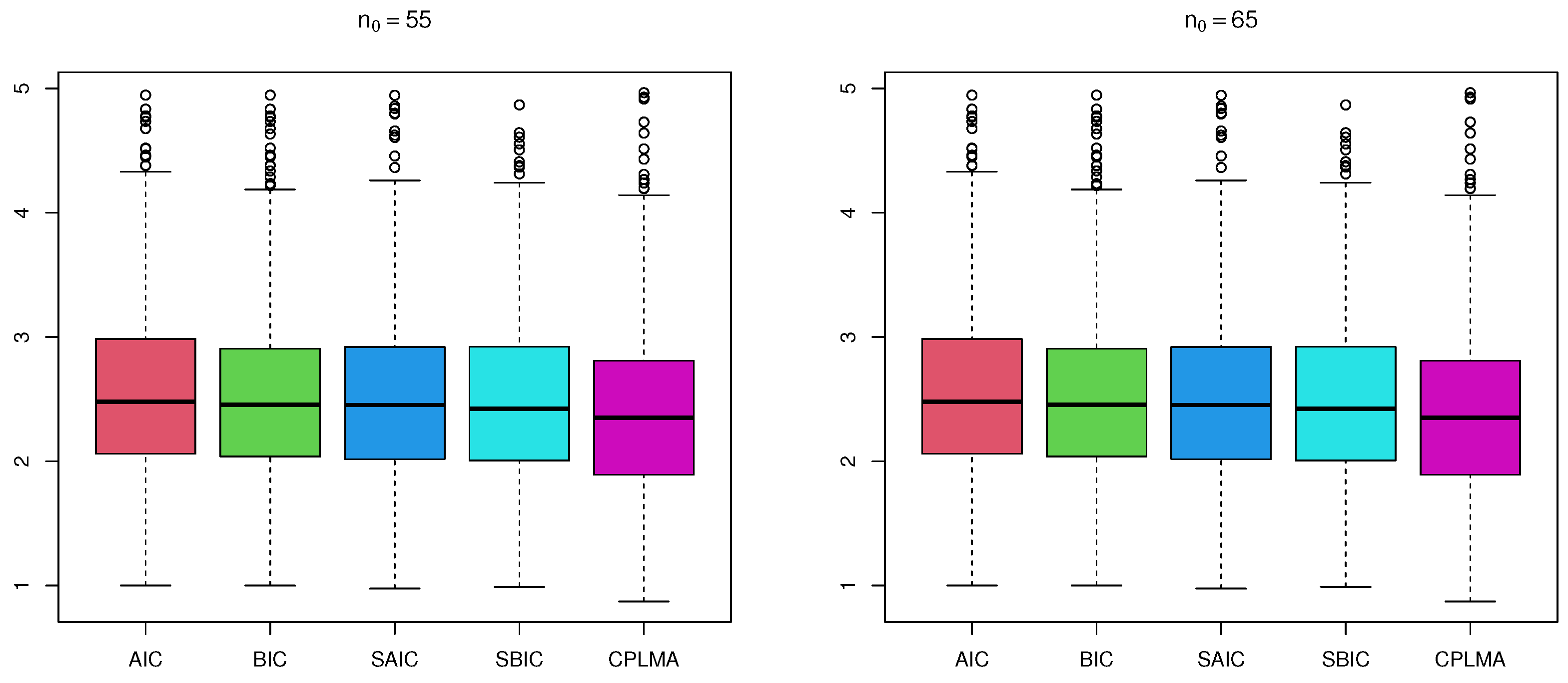
Ref. [54] found that BMI expression has a functional impact on the response variable; therefore, we establish a full PLM model with BMI expression as nonparametric variable and other covariates as linear variables. Then, we can obtain 2 5 = 32 candidate models to conduct model selection and model averaging. Let the size of training sample be n 0 = 55 or 65, and the mean and median of the RMSPE across 1000 repetitions are shown in Table 4. It can be seen from Table 4 that, both in terms of mean and median, our method CPLMA is significantly superior to other competitive methods. Figure 10 shows that the variation of MSPE for CPLMA is minor relative to that of other methods, regardless of if n 0 is 55 or 65.

7. Conclusions

In the context of the semiparametric partially linear models with censored responses, we develop a jackknife model-averaging method which selects the weights by minimizing a leave-one-out cross-validation criterion, in which the B-splines are used to approximate the nonparametric function and the least-squares estimation is applied to estimate the unknown parameters in each candidate model. The resulting model-averaging estimator, CPLMA estimator, is shown to be asymptotically optimal. A simulation study and two real data examples indicate that our method posseses some advantages over other model-selection and model-averaging methods.
Based on the results in this paper, we can further explore the optimal model averaging for the semiparametric partially linear quantile regression models with censored data. In addition, it is worthwhile to apply other optimal model-averaging methods, such as the model-averaging method based on Kullback–Leibler distance, to generalized partially linear models with censored responses.

Author Contributions

Conceptualization, W.C.; methodology, G.H., W.C. and J.Z.; software, G.H. and J.Z.; supervision, W.C. and J.Z.; writing—original draft, G.H.; writing—review and editing, J.Z. All authors have read and agreed to the published version of the manuscript.

Funding

The work of Hu is supported by the Important Natural Science Foundation of Colleges and Universities of Anhui Province (No.KJ2021A0930). The work of Zeng is supported by the Important Natural Science Foundation of Colleges and Universities of Anhui Province (No.KJ2021A0929).

Institutional Review Board Statement

Not applicable.

Informed Consent Statement

Not applicable.

Data Availability Statement

The PBC dataset is available in the R package “survival”, and the MCL dataset is available at http://llmpp.nih.gov/MCL(accessed on 18 January 2023).

Acknowledgments

The authors would like to thank the reviewers and editors for their careful reading and constructive comments.

Conflicts of Interest

The authors declare no conflict of interest.

Appendix A

To prove Theorem 1, we first give some notations which are used in the following context. Similar to L G ( ω ) and R G ( ω ) , we define the loss function of μ ˜ G ( ω ) as L ˜ G ( ω ) = μ ˜ G ( ω ) μ 2 , and the risk function as R ˜ G ( ω ) = E ( L ˜ G ( ω ) | X , U ) . Straightforward calculation yields
R ˜ G ( ω ) = A ˜ ( ω ) μ 2 + tr P ˜ ( ω ) Ω G P ˜ ( ω ) ,
where P ˜ ( ω ) = s = 1 S ω s P ˜ ( s ) , and A ˜ ( ω ) = I P ˜ ( ω ) .
Lemma A1.
Under Conditions (C.2)–(C.7), we have the following results:
sup ω W | R G ( ω ) R ˜ G ( ω ) 1 | = o p ( 1 ) ,
sup ω W | L ˜ G ( ω ) R ˜ G ( ω ) 1 | = o p ( 1 ) ,
sup ω W | L G ( ω ) R G ( ω ) 1 | = o p ( 1 ) .
Proof. 
According to the proof of (A.45), (A.48) and (A.44) in [45], we know that Equations (A2)–(A4) are satisfied. □
Lemma A2.
If Conditions (C.4)–(C.7) hold, then
sup ω W λ ¯ P ( ω ) 2 ,
sup ω W λ ¯ Λ ( ω ) = o p ( 1 ) ,
and
sup ω W λ ¯ P ˜ ( ω ) = O p ( 1 ) .
Proof. 
By the inequalities for maximum singular value, we obtain
sup ω W λ ¯ { P ( ω ) } = sup ω W λ ¯ s = 1 S ω s P ( s ) max 1 s S λ ¯ { P ( s ) } max 1 s S λ ¯ { Q ( s ) } + λ ¯ { X ˜ ( s ) ( X ˜ ( s ) X ˜ ( s ) ) 1 X ˜ ( s ) } 2 ,
where the last inequality holds because the matrices Q ( s ) and X ˜ ( s ) ( X ˜ ( s ) X ˜ ( s ) ) 1 X ˜ ( s ) are all symmetric and idempotent.
By the definition of Λ ( s ) , we have
sup ω W λ ¯ Λ ( ω ) = sup ω W λ ¯ s = 1 S ω s Λ ( s ) max 1 s S λ ¯ Λ ( s ) max 1 s S λ ¯ D ( s ) A ( s ) max 1 s S λ ¯ D ( s ) λ ¯ I P ( s ) max 1 s S λ ¯ D ( s ) 1 + λ ¯ P ( s ) max 1 s S 3 λ ¯ D ( s ) max 1 s S max 1 i n 3 ϕ i i ( s ) 1 ϕ i i ( s ) = O p p ¯ + q ¯ n ,
where the last equality is obtained based on Condition (C.6). Then, Equation (A6) is derived by Condition (C.4).
From (A5) and (A6), it can be shown that
sup ω W λ ¯ P ˜ ( ω ) max 1 s S λ ¯ P ˜ ( s ) = max 1 s S λ ¯ P ( s ) Λ ( s ) max 1 s S λ ¯ P ( s ) + max 1 s S λ ¯ Λ ( s ) 2 + O p p ¯ + q ¯ n = O p ( 1 ) .
The proof of Lemma A2 is completed. □
Lemma A3.
Assuming that Conditions (C.1), (C.2), and (C.5) are satisfied, we obtain
Z G Z G ^ n 2 = O p ( 1 ) .
Proof. 
This result is from Lemma 6.2 in [37] directly; we omit the proof procedure. □
Proof of Theorem 1. 
According to [44,45], Theorem 1 is valid if we can prove
sup ω W | R G ( ω ) R ˜ G ( ω ) 1 | = o p ( 1 ) ,
sup ω W | L ˜ G ( ω ) R ˜ G ( ω ) 1 | = o p ( 1 ) ,
sup ω W | L G ^ n ( ω ) R G ( ω ) 1 | = o p ( 1 ) ,
and
L ˜ G ( ω ^ ) inf ω W L ˜ G ( ω ) 1 = o p ( 1 ) .
By Lemma A1 and Conditions (C.2)–(C.6), Equations (A12) and (A13) are satisfied. Next, we present the proofs of (A14) and (A15), which completes the proof of Theorem 1.
For (A14), because
sup ω W | L G ^ n ( ω ) R G ( ω ) 1 | = sup ω W | μ ^ G ^ n ( ω ) μ 2 R G ( ω ) 1 | = sup ω W | μ μ ^ G ( ω ) + μ ^ G ( ω ) μ ^ G ^ n ( ω ) 2 R G ( ω ) 1 | sup ω W | L G ( ω ) R G ( ω ) 1 | + 2 sup ω W | { L G ( ω ) } 1 / 2 μ ^ G ( ω ) μ ^ G ^ n ( ω ) R G ( ω ) | + sup ω W | μ ^ G ( ω ) μ ^ G ^ n ( ω ) 2 R G ( ω ) | ,
it is sufficient to verify that
sup ω W | L G ( ω ) R G ( ω ) 1 | = o p ( 1 ) ,
and
sup ω W | μ ^ G ( ω ) μ ^ G ^ n ( ω ) 2 R G ( ω ) | = o p ( 1 ) .
Equation (A17) can be directly obtained by Lemma A1. As for (A18), by Cauchy–Schwarz inequality, we have
sup ω W | μ ^ G ( ω ) μ ^ G ^ n ( ω ) 2 R G ( ω ) | = sup ω W | P ( ω ) Z G P ( ω ) Z G ^ n 2 R G ( ω ) | ξ G 1 λ ¯ 2 P ( ω ) Z G Z G ^ n 2 4 ξ G 1 Z G Z G ^ n 2 = o p ( 1 ) ,
where the last equality follows Lemma A3 and ξ G , which is implied by Condition (C.3). Then Equation (A14) is obtained.
A simple calculation yields
C V G ^ n ( ω ) = Z G ^ n μ ˜ G ^ n ( ω ) 2 = Z G ^ n μ + μ μ ˜ G ( ω ) + μ ˜ G ( ω ) μ ˜ G ^ n ( ω ) 2 = Z G ^ n μ 2 + L ˜ G ( ω ) + Φ ( ω ) ,
where the term Z G ^ n μ 2 is unrelated to ω , and
Φ ( ω ) = μ ˜ G ( ω ) μ ˜ G ^ n ( ω ) 2 + 2 Z G ^ n Z G μ μ ˜ G ( ω ) + 2 e G A ˜ ( ω ) μ 2 e G P ˜ ( ω ) e G + 2 Z G ^ n Z G μ ˜ G ( ω ) μ ˜ G ^ n ( ω ) + 2 e G P ˜ ( ω ) Z G Z G ^ n + 2 μ μ ˜ G ( ω ) μ ˜ G ( ω ) μ ˜ G ^ n ( ω ) .
Considering (A13), (A15) is implied by
sup ω W | Φ ( ω ) | R ˜ G ( ω ) = o p ( 1 ) .
Using Cauchy–Schwarz inequality, Lemma A1, Lemma A3, and [45] to establish (A22), we only need to show
sup ω W μ ˜ G ^ n ( ω ) μ ˜ G ( ω ) 2 R ˜ G ( ω ) = o p ( 1 ) .
By Equation (A7) and Lemma A3, we observe
sup ω W μ ˜ G ^ n ( ω ) μ ˜ G ( ω ) 2 R ˜ G ( ω ) = sup ω W P ˜ ( ω ) ( Z G ^ n Z G ) 2 R ˜ G ( ω ) sup ω W λ ¯ 2 { P ˜ ( ω ) } Z G ^ n Z G 2 R ˜ G ( ω ) = o p ( 1 ) .
Thus, we can obtain (A15). This concludes the proof. □

References

  1. Engle, R.F.; Granger, C.W.J.; Rice, J.; Weiss, A. Semiparametric estimates of the relation between weather and electricity sales. J. Am. Stat. Assoc. 1986, 81, 310–320. [Google Scholar] [CrossRef]
  2. Speckman, P. Kernel smoothing in partial linear models. J. R. Stat. Soc. Ser. B Stat. Methodol. 1988, 50, 413–436. [Google Scholar] [CrossRef]
  3. Heckman, N.E. Spline smoothing in a partly linear model. J. R. Stat. Soc. Ser. B Stat. Methodol. 1986, 48, 244–248. [Google Scholar] [CrossRef]
  4. Shi, J.; Lau, T. Empirical likelihood for partially linear models. J. Multivar. Anal. 2000, 72, 132–148. [Google Scholar] [CrossRef]
  5. Härdle, W.; Liang, H.; Gao, J. Partially Linear Models; Springer Science & Business Media: Berlin, Germany, 2000. [Google Scholar]
  6. Claeskens, G.; Hjort, N.L. Model Selection and Model Averaging; Cambridge University Press: Cambridge, UK, 2008. [Google Scholar]
  7. Hansen, B.E.; Racine, J.S. Jackknife model averaging. J. Econom. 2012, 167, 38–46. [Google Scholar] [CrossRef]
  8. Racine, J.S.; Li, Q.; Yu, D.; Zheng, L. Optimal model averaging of mixed-data kernel-weighted spline regressions. J. Bus. Econ. Stat. 2022, in press. [CrossRef]
  9. Akaike, H. Statistical predictor identification. Ann. Inst. Statist. Math. 1970, 22, 203–217. [Google Scholar] [CrossRef]
  10. Schwarz, G. Estimating the dimension of a model. Ann. Statist. 1978, 6, 461–464. [Google Scholar] [CrossRef]
  11. Claeskens, G.; Hjort, N.L. The focused information criterion. J. Am. Stat. Assoc. 2003, 98, 900–916. [Google Scholar] [CrossRef]
  12. Ni, X.; Zhang, H.; Zhang, D. Automatic model selection for partially linear models. J. Multivar. Anal. 2009, 100, 2100–2111. [Google Scholar] [CrossRef] [Green Version]
  13. Raheem, S.E.; Ahmed, S.E.; Doksum, K.A. Absolute penalty and shrinkage estimation in partially linear models. Comput. Stat. Data Anal. 2012, 56, 874–891. [Google Scholar] [CrossRef]
  14. Xie, H.; Huang, J. SCAD-penalized regression in high-dimensional partially linear models. Ann. Statist. 2009, 37, 673–696. [Google Scholar] [CrossRef]
  15. Peng, J.; Yang, Y. On improvability of model selection by model averaging. J. Econom. 2022, 229, 246–262. [Google Scholar] [CrossRef]
  16. Hoeting, J.A.; Madigan, D.; Raftery, A.E.; Volinsky, C.T. Bayesian model averaging: A tutorial. Statist. Sci. 1999, 14, 382–417. [Google Scholar]
  17. Hansen, B.E. Least squares model averaging. Econometrica 2007, 75, 1175–1189. [Google Scholar] [CrossRef]
  18. Zhang, X.; Zou, G.; Carroll, R.J. Model averaging based on Kullback-Leibler distance. Stat. Sin. 2015, 25, 1583–1598. [Google Scholar] [CrossRef] [PubMed]
  19. Liu, Q.; Okui, R.; Yoshimura, A. Generalized least squares model averaging. Economet. Rev. 2016, 35, 1692–1752. [Google Scholar] [CrossRef]
  20. Gao, Y.; Zhang, X.; Wang, S.; Zou, G. Model averaging based on leave-subject-out cross-validation. J. Econom. 2016, 192, 139–151. [Google Scholar] [CrossRef]
  21. Zhang, X.; Liu, C. Model averaging prediction by K-fold cross-validation. J. Econom. 2022, in press.
  22. Lu, X.; Su, L. Jackknife model averaging for quantile regressions. J. Econom. 2015, 188, 40–58. [Google Scholar] [CrossRef]
  23. Zhang, X.; Wang, W. Optimal model averaging estimation for partially linear models. Stat. Sin. 2019, 29, 693–718. [Google Scholar] [CrossRef]
  24. Zhu, R.; Wan, A.T.K.; Zhang, X.; Zou, G. A Mallows-type model averaging estimator for the varying-coefficient partially linear model. J. Am. Stat. Assoc. 2019, 114, 882–892. [Google Scholar] [CrossRef]
  25. Xie, J.; Yan, X.; Tang, N. A model-averaging method for high-dimensional regression with missing responses at random. Stat. Sin. 2021, 31, 1005–1026. [Google Scholar] [CrossRef]
  26. Wei, Y.; Wang, Q.; Liu, W. Model averaging for linear models with responses missing at random. Ann. Inst. Statist. Math. 2021, 73, 535–553. [Google Scholar] [CrossRef]
  27. Zhang, X.; Chiou, J.; Ma, Y. Functional prediction through averaging estimated functional linear regression models. Biometrika 2018, 105, 945–962. [Google Scholar] [CrossRef]
  28. Zhang, X.; Ma, Y.; Carroll, R.J. MALMEM: Model averaging in linear measurement error models. J. R. Stat. Soc. Ser. B Stat. Methodol. 2019, 81, 763–779. [Google Scholar] [CrossRef]
  29. Ando, T.; Li, K.C. A model-averaging approach for high-dimensional regression. J. Am. Stat. Assoc. 2014, 109, 254–265. [Google Scholar] [CrossRef]
  30. Ando, T.; Li, K.C. A weight-relaxed model averaging approach for high-dimensional generalized linear models. Ann. Statist. 2017, 45, 2654–2679. [Google Scholar] [CrossRef]
  31. Zeng, D.; Lin, D. Efficient estimation for the accelerated failure time model. J. Am. Stat. Assoc. 2007, 102, 1387–1396. [Google Scholar] [CrossRef]
  32. Wang, H.J.; Wang, L. Locally weighted censored quantile regression. J. Am. Stat. Assoc. 2009, 104, 1117–1128. [Google Scholar] [CrossRef]
  33. Hjort, N.L.; Claeskens, G. Focused information criteria and model averaging for the Cox hazard regression model. J. Am. Stat. Assoc. 2006, 101, 1449–1464. [Google Scholar] [CrossRef]
  34. Du, J.; Zhang, Z.; Xie, T. Focused information criterion and model averaging in censored quantile regression. Metrika 2017, 80, 547–570. [Google Scholar] [CrossRef]
  35. Sun, Z.; Sun, L.; Lu, X.; Zhu, J.; Li, Y. Frequentist model averaging estimation for the censored partial linear quantile regression model. J. Statist. Plann. Inference 2017, 189, 1–15. [Google Scholar] [CrossRef]
  36. Yan, X.; Wang, H.; Wang, W.; Xie, J.; Ren, Y.; Wang, X. Optimal model averaging forecasting in high-dimensional survival analysis. Int. J. Forecast. 2021, 37, 1147–1155. [Google Scholar] [CrossRef]
  37. Liang, Z.; Chen, X.; Zhou, Y. Mallows model averaging estimation for linear regression model with right censored data. Acta Math. Appl. Sin. E. 2022, 38, 5–23. [Google Scholar] [CrossRef]
  38. Koul, H.; Susarla, V.; Ryzin, J.V. Regression analysis with randomly right-censored data. Ann. Statist. 1981, 9, 1276–1288. [Google Scholar] [CrossRef]
  39. Xia, X. Model averaging prediction for nonparametric varying-coefficient models with B-spline smoothing. Stat. Pap. 2021, 62, 2885–2905. [Google Scholar] [CrossRef]
  40. De Boor, C. A Practical Guide to Splines; Springer: New York, NY, USA, 2001. [Google Scholar]
  41. Kaplan, E.L.; Meier, P. Nonparametric estimation from incomplete observations. J. Am. Stat. Assoc. 1958, 53, 457–481. [Google Scholar] [CrossRef]
  42. Hu, G.; Cheng, W.; Zeng, J. Model averaging by jackknife criterion for varying-coefficient partially linear models. Comm. Statist. Theory Methods 2020, 49, 2671–2689. [Google Scholar] [CrossRef]
  43. Turlach, B.A.; Weingessel, A.; Moler, C. Quadprog: Functions to Solve Quadratic Programming Problems. R Package Version 1.5-8. 2019. Available online: https://CRAN.R-project.org/package=quadprog (accessed on 16 December 2022).
  44. Wei, Y.; Wang, Q. Cross-validation-based model averaging in linear models with response missing at random. Stat. Probab. Lett. 2021, 171, 108990. [Google Scholar] [CrossRef]
  45. Zhang, X.; Wan, A.T.K.; Zou, G. Model averaging by jackknife criterion in models with dependent data. J. Econom. 2013, 174, 82–94. [Google Scholar] [CrossRef]
  46. Wan, A.T.; Zhang, X.; Zou, G. Least squares model averaging by Mallows criterion. J. Econom. 2010, 156, 277–283. [Google Scholar] [CrossRef]
  47. Fan, J.; Ma, Y.; Dai, W. Nonparametric independence screening in sparse ultra-high-dimensional varying coefficient models. J. Am. Stat. Assoc. 2014, 109, 1270–1284. [Google Scholar] [CrossRef] [PubMed]
  48. Bates, D.M.; Venables, W.N. Splines: Regression Spline Functions and Classes. R Package Version 3.6-1. 2019. Available online: https://CRAN.R-project.org/package=splines (accessed on 15 December 2022).
  49. Therneau, T.M.; Lumley, T.; Elizabeth, A.; Cynthia, C. Survival: Survival Analysis. R Package Version 3.4-0. 2022. Available online: https://CRAN.R-project.org/package=survival (accessed on 15 December 2022).
  50. Tibshirani, R. The lasso method for variable selection in the Cox model. Stat. Med. 1997, 16, 385–395. [Google Scholar] [CrossRef]
  51. Shows, J.H.; Lu, W.; Zhang, H.H. Sparse estimation and inference for censored median regression. J. Statist. Plann. Inference 2010, 140, 1903–1917. [Google Scholar] [CrossRef] [PubMed]
  52. Diebold, F.X.; Mariano, R.S. Comparing predictive accuracy. J. Bus. Econ. Stat. 1995, 13, 253–263. [Google Scholar]
  53. Rosenwald, A.; Wright, G.; Wiestner, A.; Chan, W.C.; Connors, J.M.; Campo, E.; Gascoyne, R.D.; Grogan, T.M.; Muller-Hermelink, H.K.; Smeland, E.B.; et al. The proliferation gene expression signature is a quantitative integrator of oncogenic events that predicts survival in mantle cell lymphoma. Cancer Cell 2003, 3, 185–197. [Google Scholar] [CrossRef] [PubMed]
  54. Ma, S.; Du, P. Variable selection in partly linear regression model with diverging dimensions for right censored data. Stat. Sin. 2012, 22, 1003–1020. [Google Scholar] [CrossRef] [Green Version]
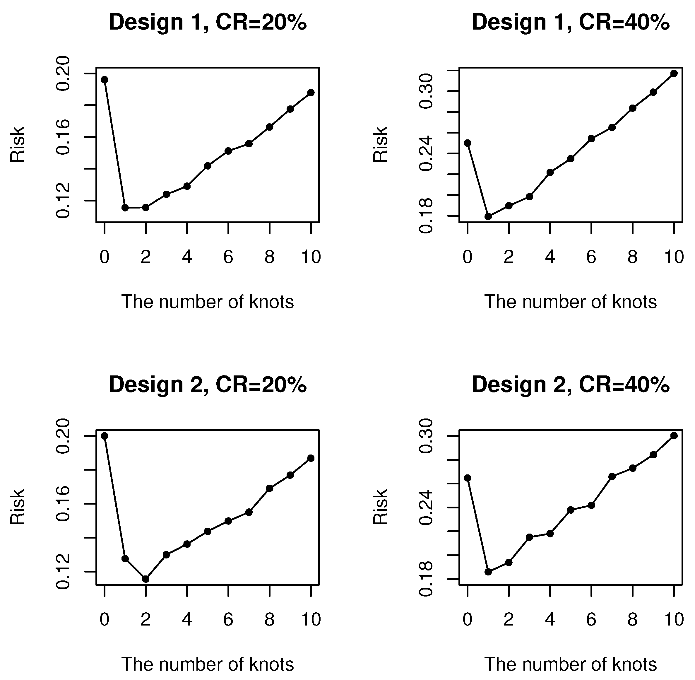
Figure 1. The curves of the mean of risk with the number of knots over 500 replications.
Mathematics 11 00734 g001
Figure 2. Risk comparisons for Design 1 when α = 2 and the censoring rate is about 20 % .
Mathematics 11 00734 g002
Figure 3. Risk comparisons for Design 1 when α = 0.5 and the censoring rate is about 20 % .
Mathematics 11 00734 g003
Figure 4. Risk comparisons for Design 1 when α = 2 and the censoring rate is about 40 % .
Mathematics 11 00734 g004
Figure 5. Risk comparisons for Design 1 when α = 0.5 and the censoring rate is about 40 % .
Mathematics 11 00734 g005
Figure 6. Risk comparisons for Design 2 when α = 2 and the censoring rate is about 20 % .
Mathematics 11 00734 g006
Figure 7. Risk comparisons for Design 2 when α = 0.5 and the censoring rate is about 20 % .
Mathematics 11 00734 g007
Figure 8. Risk comparisons for Design 2 when α = 2 and the censoring rate is about 40 % .
Mathematics 11 00734 g008
Figure 9. Risk comparisons for Design 2 when α = 0.5 and the censoring rate is about 40 % .
Mathematics 11 00734 g009
Figure 10. Boxplots for MSPEs of five methods for the MCL data.
Mathematics 11 00734 g010
Table 1. The basic notations used in this paper.
NotationsDescriptions
T i The survival time of the ith subject
Y i The response variable, a transformation of T i
X i The covariate vector of the ith subject
δ i The censoring indicator of the ith subject
C i The last follow up time of the ith subject
Z i The observed time, equal to min ( Y i , C i )
G ( · ) The cumulative distribution function of C i
Z G n × 1 synthetic response vector
μ n × 1 conditional mean vector of the response
B ( s ) n × k n B-spline basis matrix for the sth model
β ( s ) p s × 1 linear regression coefficient vector for the sth model
α ( s ) k n × 1 spline coefficient vector for the sth model
G ^ n ( · ) The Kaplan–Meier estimator of G ( · )
β ^ G , ( s ) The estimator of β ( s ) with G ( · )
α ^ G , ( s ) The estimator of α ( s ) with G ( · )
μ ^ G , ( s ) The estimator of μ for the sth model with G ( · )
μ ^ G ( ω ) The model-averaging estimator of μ with G ( · )
μ ˜ G , ( s ) or μ ˜ G ^ n , ( s ) the sth jackknife estimator of μ with G ( · ) or G ^ n ( · )
μ ˜ G ( ω ) or μ ˜ G ^ n ( ω ) the jackknife model-averaging estimator of μ with G ( · ) or G ^ n ( · )
Table 2. The mean and median of RMSPE across 1000 repetitions.
n 0 MethodBICSAICSBICCPLMA
140mean1.0050.9870.9830.979
median1.0140.9920.9950.987
160mean1.0050.9870.9830.982
median1.0060.9860.9880.984
180mean1.0110.9910.9910.986
median1.0110.9900.9900.981
200mean1.0140.9930.9950.989
median1.0120.9840.9900.976
220mean1.0120.9950.9970.994
median1.0200.9941.0030.993
240mean1.0080.9950.9980.993
median1.0170.9960.9990.988
Table 3. Diebold–Mariano test results for the differences in MSPE.
n 0 Method AIC BIC AIC SAIC AIC SBIC AIC CPLMA BIC SAIC BIC SBIC BIC CPLMA SAIC SBIC SAIC CPLMA SBIC CPLMA
140DM−3.01315.13012.33514.85816.74325.34116.6334.9736.3612.834
p-value0.0030.0000.0000.0000.0000.0000.0000.0000.0000.005
160DM−3.01416.60712.49014.86217.19630.33118.4744.9955.5380.942
p-value0.0030.0000.0000.0000.0000.0000.0000.0000.0000.347
180DM−8.08212.3557.87411.23822.55434.56121.914−0.3484.4395.679
p-value0.0000.0000.0000.0000.0000.0000.0000.7280.0000.000
200DM−11.47312.3204.74411.39323.96232.28622.550−3.7215.2888.690
p-value0.0000.0000.0000.0000.0000.0000.0000.0000.0000.000
220DM−9.5098.5002.3085.58719.00422.31617.152−4.0111.0855.059
p-value0.0000.0000.0210.0000.0000.0000.0000.0000.2780.000
240DM−5.4847.3321.4415.84812.90115.42712.998−4.1752.1106.561
p-value0.0000.0000.1500.0000.0000.0000.0000.0000.0350.000
Table 4. The mean and median of RMSPE across 1000 repetitions.
n 0 MethodBICSAICSBICCPLMA
55mean1.0110.9820.9880.923
median0.9510.9650.9370.918
65mean0.9920.9760.9870.947
median0.9820.9700.9730.939
Disclaimer/Publisher’s Note: The statements, opinions and data contained in all publications are solely those of the individual author(s) and contributor(s) and not of MDPI and/or the editor(s). MDPI and/or the editor(s) disclaim responsibility for any injury to people or property resulting from any ideas, methods, instructions or products referred to in the content.