Article

Dynamic Analysis and FPGA Implementation of a New, Simple 5D Memristive Hyperchaotic Sprott-C System

1
School of Computer and Communication Engineering, Changsha University of Science and Technology, Changsha 410114, China
2
College of Computer Science and Electronic Engineering, Hunan University, Changsha 410082, China
3
Hunan Post & Telecommunication Planning and Designing Institute, No. 236 Yuanda Road, Changsha 410126, China
*
Author to whom correspondence should be addressed.
Mathematics 2023, 11(3), 701; https://doi.org/10.3390/math11030701
Submission received: 30 December 2022 / Revised: 21 January 2023 / Accepted: 25 January 2023 / Published: 30 January 2023
(This article belongs to the Special Issue Chaotic Systems and Their Applications)

Abstract

:
In this paper, we first present a simple seven-term 4D hyperchaotic system based on the classical Sprott-C 3D chaotic system. This novel system is inspired by the simple 4D hyperchaotic system based on Sprott-B proposed by A. T. Sheet (2022). We discuss the phenomenon of premature divergence brought about by the improper choice of coupling parameters in that paper and describe the basic properties of the new system with phase diagrams, Lyapunov exponential spectra and bifurcation diagrams. Then, we find that the dynamical behaviors of the system suffer from the limitation of the control parameters and cannot represent the process of motion in detail. To improve the system, we expand the dimensionality and add the control parameters and memristors. A 5D memristive hyperchaotic system with hidden attractors is proposed, and the basic dynamical properties of the system, such as its dissipation, equilibrium point, stability, Lyapunov exponential spectra and bifurcation diagram, are analyzed. Finally, the hardware circuits of the 4D Sprott-C system and the 5D memristive hyperchaotic system were realized by a field programmable gate array (FPGA) and verified by an experiment. The experimental results are consistent with the numerical simulation results obtained in MATLAB, which demonstrates the feasibility and potential of the system.

1. Introduction

In recent decades, chaos theory has made rapid developments. Chaotic systems have been widely studied and used in neural networks [1,2,3], neurons [4,5,6], system synchronization [7,8,9], secure communications [10,11,12], image encryption [13,14,15], bioengineering [16,17,18] and other fields [19,20,21]. The chaotic signal is an ideal choice for secure communication because of its concealment, unpredictability, high complexity and easy realization. To improve the complexity of chaos, various chaotic systems and networks with complex dynamic characteristics have been proposed in recent years [22,23,24,25].
In 1994, J. C. Sprott constructed 19 differentsystems with nonlinear quadratic terms and found abundant chaotic phenomena [26]. Since the parameters of all the systems in [26] are determined, many people have improved them in recent years and obtained rich results. For example, the generalized Sprott-C system with only two stable equilibrium points was studied in [27]. In [28], an extended Sprott-E system was introduced for the new system through a general quadratic control scheme with three arbitrary parameters. It can be seen that it is still meaningful and promising to improve the Sprott system and study the chaotic characteristics of the system.
Compared with general chaotic systems, high-dimensional hyperchaotic systems have more complex attractor topology and dynamic behavior. It will be safer to apply high-dimensional hyperchaotic systems to encryption of communications [29,30,31]. High-dimensional hyperchaotic systems have always been the focus of chaos theory research [32,33,34]. In [32], a five-dimensional (5D) hyperchaotic system was constructed, the states of the system under different parameters were studied and the complexity of the system was analyzed. A new 4D multi-scroll hyperchaotic system was constructed in [33]. By studying the dynamic characteristics of the system, it was proved that the system has complex behavior. An innovative method with analytical and numerical aspects was proposed in [34], which can generate a class of hyperchaotic attractors with multiple wings and different shapes. The construction of hyperchaotic systems with complex dynamics based on the Sprott system has also attracted the attention of scholars. In [35], a 4D simple hyperchaotic system is established by linear state feedback control from the famous Sprott-S system. In [36], a 5D hyperchaotic Sprott-B system with hidden attractors was proposed. The system has ten terms, including two quadratic nonlinearities and one control parameter.
In 1971, Leon Chua predicted the existence of the fourth fundamental circuit element, namely, the memristor, based on the relationship between magnetic flux and electric charge. As a nonlinear circuit component, the memristor is considered an organic link between the magnetic and electric fields [37,38]. Its resistance can be changed by adjusting voltage or current. It is an ideal device for designing chaotic and hyperchaotic systems [39,40,41]. In [42], by adding a flux-controlled memristor with the linear memristor to a four-wing Chen system, a new 4D four-wing memristive hyperchaotic system was constructed. In [43], a new kind of non-equilibrium memristive hyperchaotic system is studied, which is generated by the extended diffusionless Lorenz equation. Recently, the higher-dimensional memristive hyperchaotic system has also become a research hotspot. A 5D memristive exponential hyperchaotic system was proposed in [44]. The system shows rich dynamic behaviors, including the coexistence of multiple attractors. In [45], a 5D memristive hyperchaotic system was proposed by introducing a quadratic nonlinear memristor into the existing 4D chaotic system as a feedback term.
The memristive Sprott system has also been studied. In 2022, Ramamoorthy et al. proposed and studied the dynamic behavior of a new memristive chaotic Sprott-B system. This system has a bias term that can adjust the symmetry of the proposed model, resulting in homogeneous and heterogeneous behavior [46]. Although the system shows complex dynamic behavior, it is not a hyperchaotic system. By comparing the literature on memristive hyperchaotic systems [42,43,44,45], in recent years, it has been found that these hyperchaotic systems have many mathematical terms and complex structures, and there are few reports on the research of memristive hyperchaotic Sprott systems.
Most new chaotic systems use discrete components to design analog circuits to generate analog chaotic signals. Analog components are extremely unstable and vulnerable to external influences. The modern digital signal processing technology is used to achieve continuous chaotic signals, which can make the generated chaotic attractors stable and reliable, and less affected by external factors [47,48]. FPGA is widely used in modern digital signal processing because of its large capacity, high density and reliability. In recent years, many researchers have used FPGA to implement complex chaotic systems [49,50,51,52,53,54,55,56,57]. The FPGA implementation of two multi-scroll chaotic oscillators was proposed in [50]. In [52], three different algorithms (Euler, Heun and RK4) were used for the first time to realize a real-time novel chaotic oscillator through FPGA. In [55], an autonomous chaotic system with hidden attractors and coexistence attractors was implemented using FPGA.
In this paper, a new, simple, 4D, seven-term hyperchaotic system with self-excited attractors is constructed based on the Sprott-C system, and the attractor’s divergence due to the inappropriate parameter selection of the simple hyperchaotic system is discussed. The solution is also proposed. Then, a 5D memristive hyperchaotic system with hidden attractors is proposed based on the new system, which compensates for the incompleteness of the nonlinear motion of the 4D system due to the limitation of the control parameters. The system has fewer parameters and is more concise than general memristive hyperchaotic systems, but dynamic behaviors of the system are complex. It meets the second criterion proposed by Sprott: "the system should exhibit some previously unobserved behavior." Finally, the hardware circuit of the new memristive system is designed, and it was implemented. The experimental results are consistent with the numerical simulation’s results. It is proved that the system is a continuous equilibrium point and a hidden hyperchaotic system with superior convenience, and it is also realizable.
The rest of this work is structured as follows. In Section 2, a mathematical model of a seven-term, 4D, simple hyperchaotic system based on the Sprott-C system is presented and analyzed for equilibrium points, stability and dynamical behavior. In Section 3, a 5D memristive hyperchaotic system with the hidden attractor is constructed by refining the 4D system, adding a memristive function, coupling parameters and expanding the dimensionality. Through numerical calculations and graphic description, its dynamics were analyzed, and the coexistence of the system was studied. In Section 4, actual FPGA-based digital circuits for both models are presented, and the experimental results agree with the oscilloscope display, hardware experimental results and MATLAB simulations. Finally, the conclusions of this work are given in Section 5.

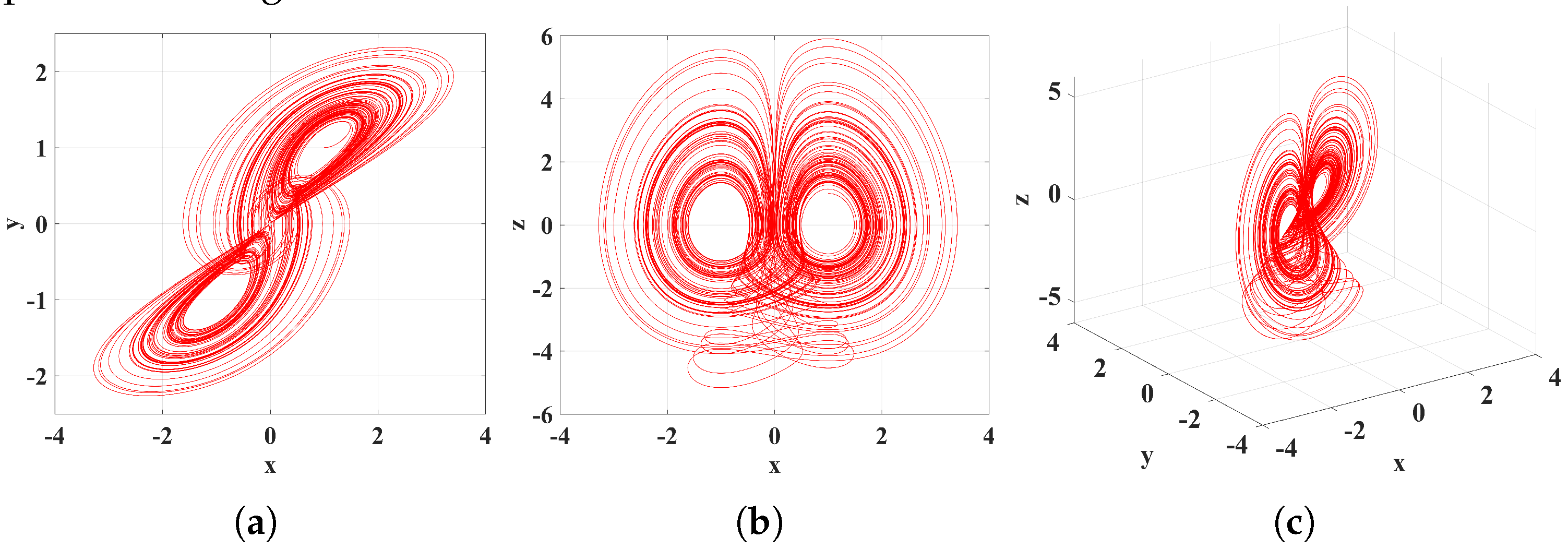
2. A Simple 4D Hyperchaotic System

J. C. Sprott discovered the very classical Sprott series [26] of 19 kinds of simple 3D chaotic systems in 1994. Researchers usually construct new systems by coupling based on these simple systems. In 2022, A. T. Sheet [58] proposed a simple hyperchaotic system based on the Sprott-B system. It is pointed out in the article that when the control parameters ( a , b ) = ( 0.1 , 0.09 ) and I C = ( 0.3 , 0.2 , 0.3 , 0.1 ) , the system is hyperchaotic. Additionally, for the chaotic attractor in the x u plane, when duration T = 1000 , as in Figure 1a, it is obvious that the system attractors diverge quickly, making it impossible to discretize the system and realize the potential of chaotic digital circuits or secure communication. Hence, values of the system are inappropriate. This will not happen when b takes a small positive or any negative number. The final solution is to limit the value of b to a negative number. Based on the above considerations, this paper proposes a simple hyperchaotic system with the same seven terms, two nonlinear terms, and two control parameters based on the Sprott-C system as:
x ˙ = y z y ˙ = x y z ˙ = 1 x x u ˙ = a x + b u
where a and b are coupling parameters. Considering the divergence:
V = x ˙ x + y ˙ y + z ˙ z + u ˙ u = b 1
When b = 1 , system (1) is a conservative system. When b < 1 , system (1) is a dissipative system.
In this paper, only the dissipative system is taken into account. Based on avoiding the rapid divergence of attractors, the values of b are always less than 0. In this paper, the default coupling parameter a is greater than 0, and two stable equilibrium points are obtained when b is less than 0 and duration T = 5000 , with part of the transient time being removed. Two-dimensional attractors of the x y plane and the x z plane and a 3D attractor of the x y z plane are shown in Figure 1b–d.

2.1. Equilibrium Point and Stability

In the system (1), let x ˙ = y ˙ = z ˙ = u ˙ = 0 . The equilibrium points can be expressed as:
E = x * = ± 1 , y * = ± 1 , z * = 0 , u * = a b
The default a is positive, and b is negative, thereby determining that the system (1) has two conjugate equilibrium points. We determine the stability of the equilibrium points by determining the eigenvalues from the Jacobi matrix.
J = 0 z y 0 1 1 0 0 2 x 0 0 0 a 0 0 b
By bringing Equation (3) into Equation (4), we will get:
J 1 / 2 = 0 0 ± 1 0 1 1 0 0 2 0 0 0 a 0 0 b
J 1 and J 2 have the same characteristic equation:
( b λ ) ( 1 λ ) λ 2 + 2 = 0
The roots are obtained by the MATLAB solution:
λ 1 = b λ 2 = 1 λ 3 = 1.414 i λ 4 = 1.414 i
When all the eigenvalues are imaginary, the equilibrium points are the central fixed points. However, only the third and fourth eigenvalues are pure imaginary numbers. They are only responsible for the rotation and have no effect on stability, which is determined by the first and second eigenvalues. One of the eigenvalues is negative, and b can be a very small positive number or any negative number. When b is positive, the equilibrium points are unstable. When b is negative, the equilibrium points are stable. In this paper, the default parameter b is negative, so it is judged that the two equilibrium points of system (1) are stable fixed points.

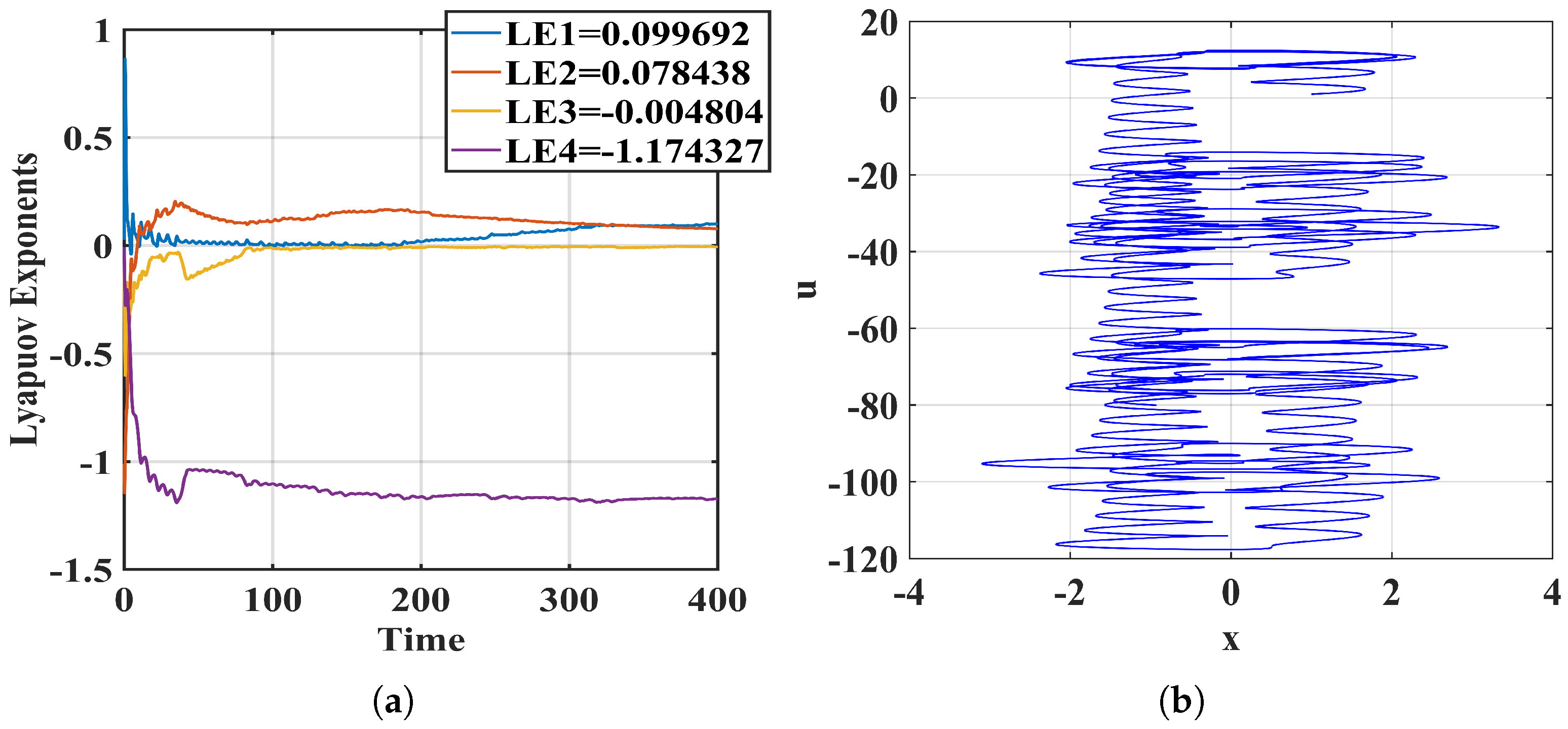
2.2. Lyapunov Exponents

The Lyapunov exponent (LE) represents the numerical characteristics of the average exponential dispersion rate of adjacent trajectories in phase space. It is also known as the Lyapunov characteristic index. Lyapunov exponents are one of the important tools used to classify the behavior of dynamical systems as chaotic or hyperchaotic. The general basis for discerning whether it is chaotic or not is by the positive or negative Lyapunov characteristic exponents; with one positive exponent, the system is chaotic, and with two or more positive exponents, the system is hyperchaotic. It takes into account the maximum quantum Kaplan–Yorke dimension as a way to judge the complexity of the system. The simulations in this paper were all performed by the mathematical software (MATLAB2017a), measured by the numerical method of ODE45.
Measurements were performed for system (1). By setting ( a , b ) = ( 1 , 0.001 ) , ( x 0 , y 0 , z 0 , u 0 ) = ( 1 , 1 , 1 , 1 ) and taking Δ t = 0.01 , with T = 400 , the final measured Lyapunov exponents are:
L E 1 = 0.099692 L E 2 = 0.078438 L E 3 = 0.004804 L E 4 = 1.174328 i = 1 4 L E i = 1.001
The absolute values of the first two positive Lyapunov exponents are much greater than the absolute value of the third negative Lyapunov exponent. Thus, the state of the system is hyperchaotic. The four exponents obtained from the corresponding initial values ( 1 , 1 , 1 , 1 ) and control parameters ( 1 , 0.001 ) sum to approximately equal −1.001, corresponding to the divergence ( b 1 ) obtained from Equation (2). The Lyapunov exponent diagram (Figure 2a) and the attractor diagram (Figure 2b) at this point are given. At this time, the attractor in the x u plane resembles a spring-like attractor that is clearly chaotic in form and does not diverge away quickly. The Lyapunov dimension (Kaplan–Yorke dimension) of the attractor of the system (1) is calculated as:
D L E = j + 1 L E j + 1 i = 1 j L E i D L E = 3 + L E 1 + L E 2 + L E 3 L E 4 = 3 + 0.1740 = 3.1740

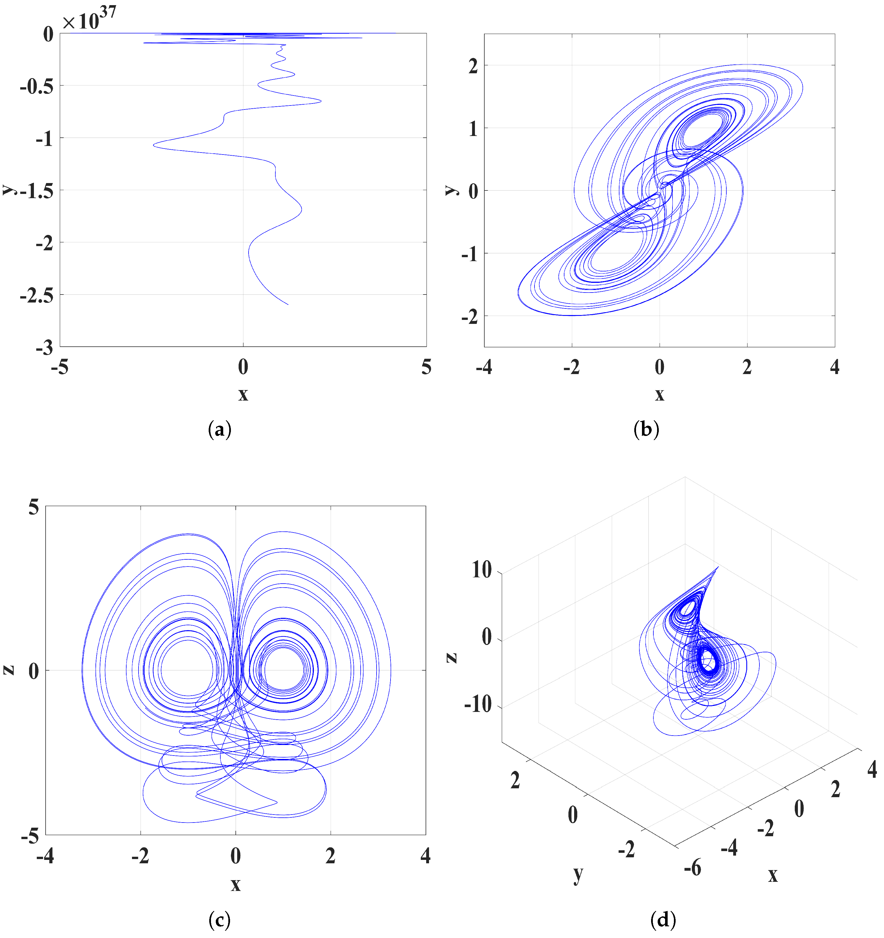
2.3. Nonlinear Dynamic Behavior Analysis

Bifurcation refers to a sudden change in the nature or topology of the system caused by small and continuous changes in control parameters. It is often used to describe the change in the number of stable points of the system. When the initial conditions I C = ( 0.1 , 0.1 , 0.1 , 0.1 ) are set, a change in the essence of the nonlinear system is observed with a fixed control parameter a or a fixed parameter b. It can be observed that system (1) is always in the chaotic or hyperchaotic state from Figure 3a,b, and no periodic change can be observed. This phenomenon is caused by the pursuit of system simplification without setting parameters for nonlinear terms, which leads to the failure to observe the change in system topology.
The Lyapunov exponent measures the degree of separation of a system with time (iteration) due to a small initial error. When the bifurcation diagram cannot describe the system’s change, it can be judged by the Lyapunov exponent or Lyapunov exponent spectrum. We prepared Lyapunov exponent spectra to observe the dynamical behaviors of the system (1) and used two sets of initial values: ( 0.1 , 0.1 , 0.1 , 0.1 ) and ( 1 , 1 , 1 , 1 ) . We fixed one control parameter and observed the variation in the other control parameter in the Lyapunov exponent spectrum in the range of 10. To avoid divergence, we restricted b to be always less than 0. In the software, when performing the simulation, we took a step size of 1 and a time range of 700.
(1) Set the initial value to ( 0.1 , 0.1 , 0.1 , 0.1 ) . First, we fixed the control parameter b as −0.01, and the control parameter a changed to [ 0 , 10 ] . It can be observed from Figure 4a that system (1) is always in a chaotic state and very stable, and no periodic state or hyperchaotic state was observed. Then, we fixed the control parameter a as 0.1 , and the control parameter b changed within [ 10 , 0 ] . It can be observed from Figure 4b that system (1) is also always chaotic, and the topological structure does not change.
(2) Set the initial value to ( 1 , 1 , 1 , 1 ) . First, we fixed the control parameter b to −0.01 and the control parameter a to vary in [ 0 , 10 ] . As can be shown in Figure 4c, system (1) is always in a hyperchaotic state, as presented in the bifurcation diagram, and again, no periodic or chaotic state can be observed. Finally, we fixed the control parameter a to be 0.1 and the control parameter b to vary within [ 10 , 0 ) , as can be observed in Figure 4d. However, Lyapunov exponents always have two positive numbers within [ 10 , 0.1 ] . The two negative exponents of the Lyapunov exponent spectrum are much larger than the two positive exponents. Only when b [ 0.1 , 0 ] does one negative exponent of system (1) approache zero, and system (1) is in a hyperchaotic state. However, from the Lyapunov exponent spectrum as a whole, the topology of the system also does not change.
The reason for ( 1 ) and ( 2 ) is that system (1) pursues streamlining and reduces the degree of coupling, making the system very homogeneous in terms of changes, and this is where the system needs to be improved.

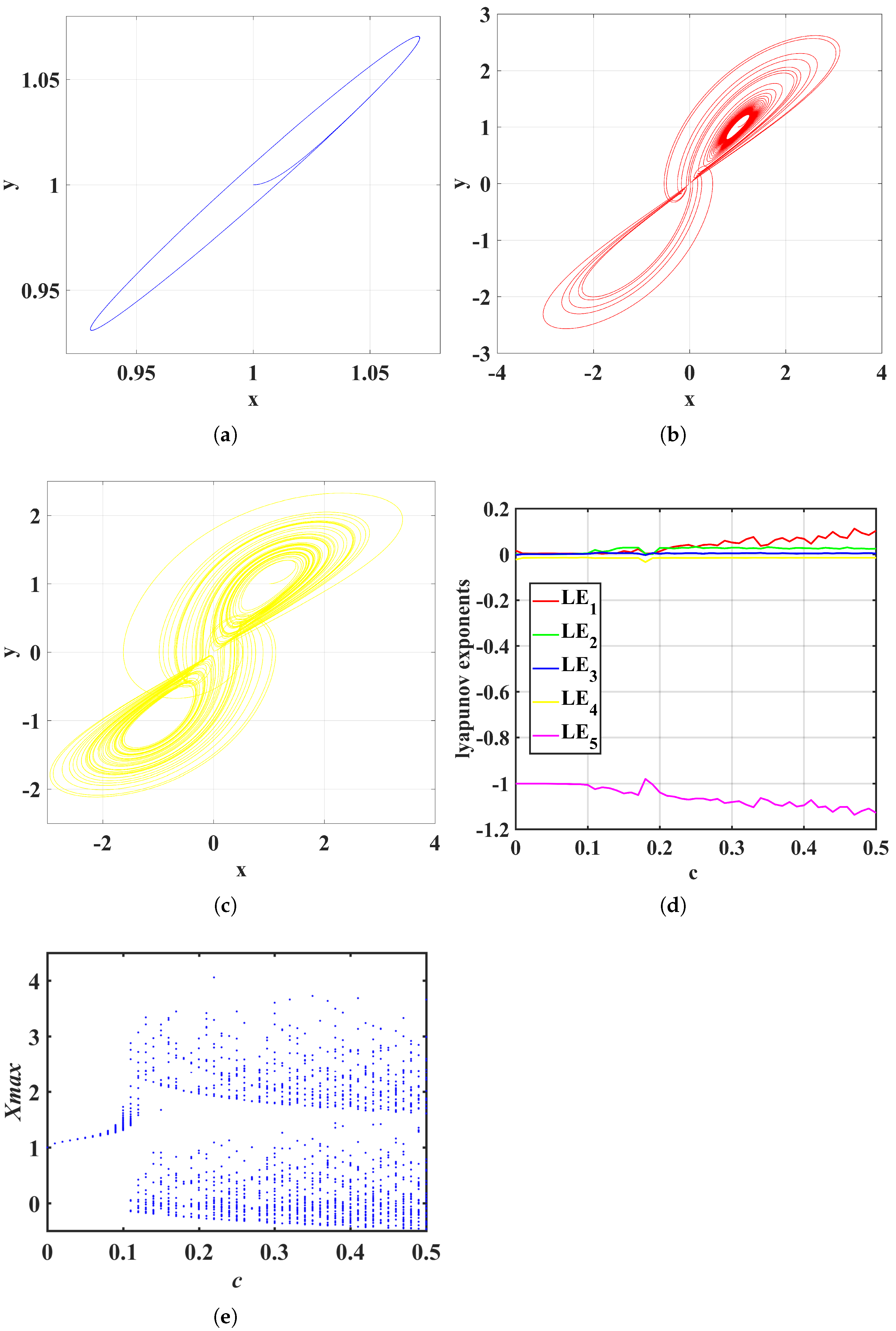
3. Sprott-C Hyperchaotic System Based on Memristor

A memristor is a circuit device representing the relationship between magnetic flux and charge, and it is widely used in chaotic circuits. It can realize chaotic oscillation signals and increase the complexity of the system. In order to perfect the system, based on system (1), proposed in the second part, the dimensions are expanded, the control parameters are increased, and a memristor with nonlinear flux control is added at an appropriate position so that the system becomes a 5D memristive hyperchaotic system, which has countless equilibrium points and is classified as the hidden attractor. The formula is as follows:
x ˙ = c y z y ˙ = x y z ˙ = 1 x x u ˙ = a x b u + k W ( φ ) z φ ˙ = y x
where x , y , z , u , φ are state variables; and a , b , c , and k are system control parameters—all are positive. The system has been fine-tuned to avoid divergence, so b is also positive. k represents the strength of a memristor, and W ( φ ) is a memristor, defined as W ( φ ) = d q ( φ ) / d ( φ ) . The memory inductance is determined as:
W ( φ ) = d q ( φ ) d ( φ ) = m + 3 n φ 2
Additionally, m and n are set as two positive parameters, which makes the magnetically controlled memristor easier to complete. Currently, many researchers use smooth flux control to build many chaotic oscillators with complex dynamic characteristics. When ( a , b , c , k , m , n ) are ( 2 , 0.01 , 0.5 , 5 , 0.1 , 0.01 ) and initial conditions are ( 1 , 1 , 1 , 1 , 1 ) , see the phase diagrams of the x z plane, the x u plane and the 3D phase diagram of the x y z plane from Figure 5a–c:

3.1. Divergence and Lyapunov Exponents

Consider the divergence:
V = x ˙ x + y ˙ y + z ˙ z + u ˙ u + φ ˙ φ = b 1
When b = 1 , system (10) is conservative. When b > 1 , system (10) is a dissipative system. Over time, the system will eventually shrink to an attractor with zero volume.
First, fix the initial values I C = ( 1 , 1 , 1 , 1 , 1 ) . The control parameters ( a , b , c , k , m , n ) are ( 0.71 , 0.001 , 2.1 , 0.1 , 0.1 , 0.01 ) . Consider the Lyapunov exponent and the largest quantum Kaplan–Yorke dimension. This work was carried out in mathematical software (MATLAB2017a) and was calculated by the numerical method of ODE45. The step length was 0.01, and the time range was 400. Finally, the measured Lyapunov exponents were:
L E 1 = 0.095916 L E 2 = 0.081339 L E 3 = 0.002892 i = 1 5 L E i = 1.001 L E 4 = 0.001059 L E 5 = 1.180088
It can be seen that when the fourth and the third exponents closest to zero are taken as zero, there are still two positive numbers in the Lyapunov exponent, and the system is in a hyperchaotic state. At this time, the quantum Kaplan–Yorke dimension is:
D L E = j + 1 L E j + 1 i = 1 j L E i D L E = 4 + L E 1 + L E 2 + L E 3 + L E 4 L E 5 4.1792

3.2. Equilibrium Points and Stability

In the system (11), let x ˙ = y ˙ = z ˙ = u ˙ = φ ˙ = 0 , and the following equation is obtained.
y z = 0 x y = 0 1 x x = 0 a x b u + k ( m + 3 n φ φ ) z = 0 y x = 0
Through calculation, the equilibrium point can be expressed as:
E = x * = ± 1 , y * = ± 1 , z * = 0 , u * = ± a b , φ * R
φ can take on any value. Obviously, the system consists of countless equilibrium points. As the stability of the equilibrium point of the system is affected by the value of φ , it will not be discussed.

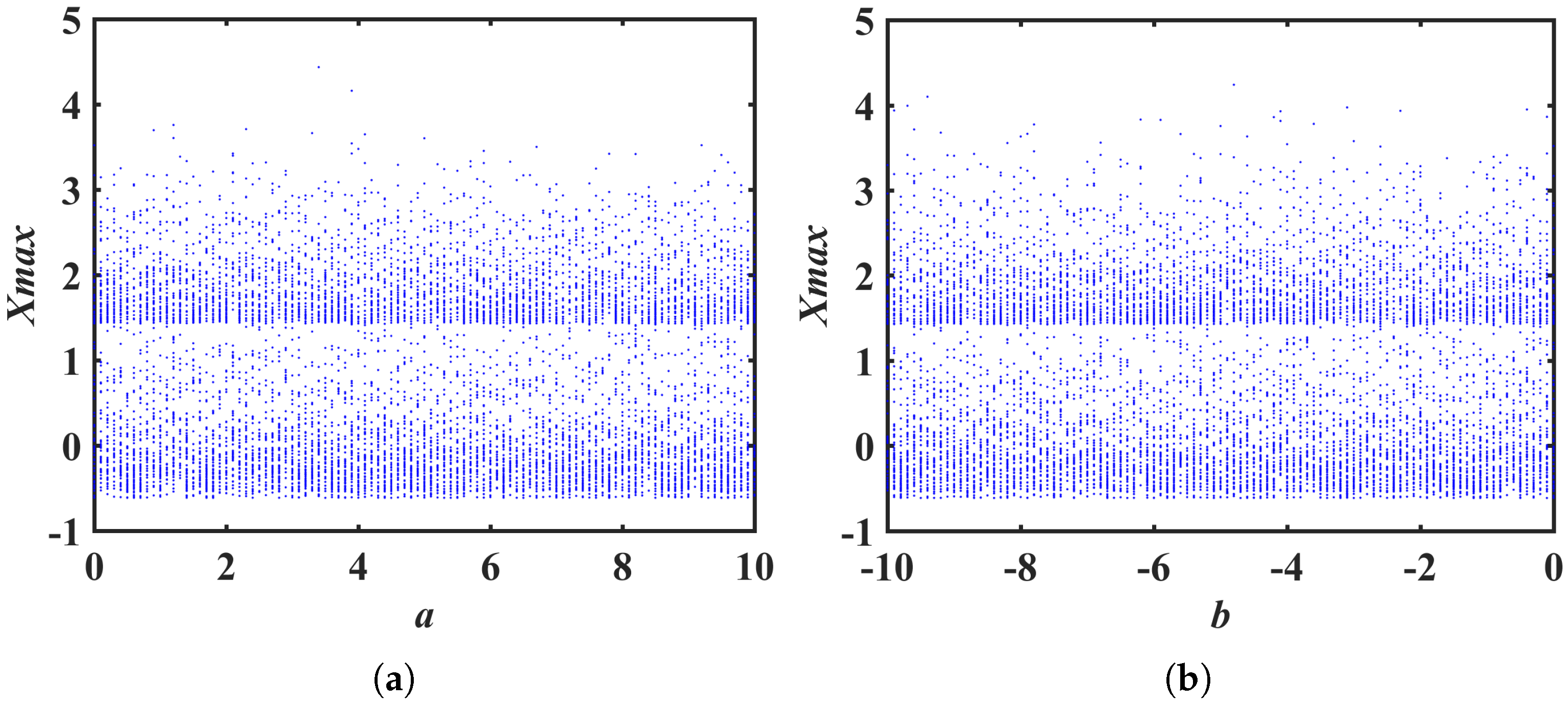
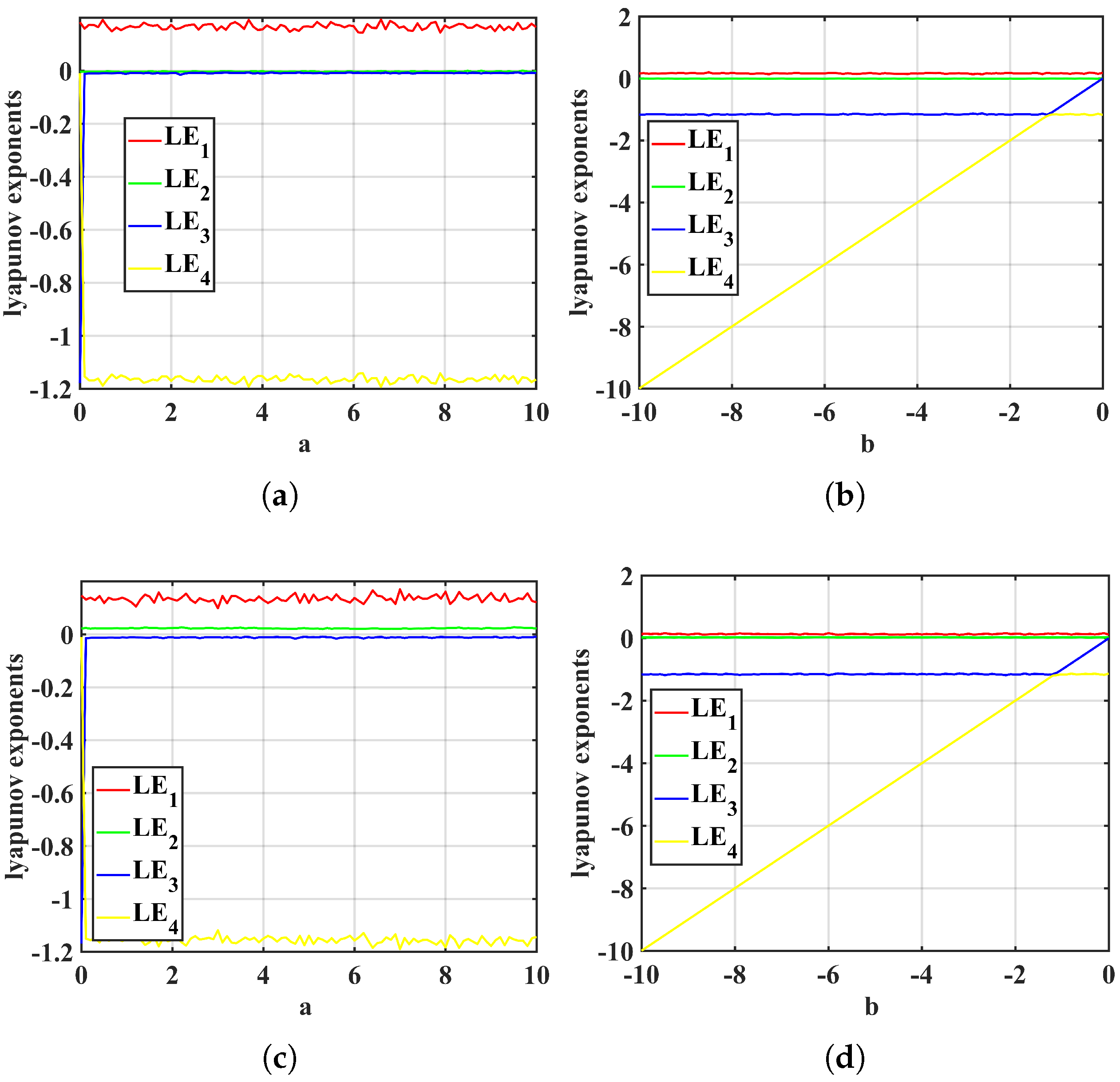
3.3. Abundant Dynamic Behavior

Bifurcation is a unique phenomenon among nonlinear phenomena, which refers to a sudden change in system topology caused by parameter changes in the nonlinear dynamic system. It is often used to describe the structural transformation of a chaotic system. The phase diagram describes the relationship between system variables and can be used to reflect the current state and movement process of the system. In this section, the bifurcation diagram, phase diagrams and the Lyapunov exponent spectrum are used to describe the dynamic behavior of the system.
When the initial values are set to ( 1 , 1 , 1 , 1 , 1 ) , the fixed control parameters ( a , b , k , m , n ) are ( 1 , 0.01 , 5 , 0.1 , 0.01 ) so that the control parameter c changes within ( 0 , 0.5 ] , and the system will show a periodic state, a chaotic state and a hyperchaotic state. When c ( 0 , 0.1 ] , system (10) is in a periodic state, the x y plane attractor is shown in Figure 6a—the color is blue. When c ( 0.1 , 0.13 ] , the system (10) will change from the periodic state to the chaotic state, as shown in Figure 6b—the color is red. When c ( 0.13 , 0.175 ] , it will change from the chaotic state to the hyperchaotic state. When c ( 0.175 , 0.19 ] , system (10) enters the periodic state. When c ( 0.19 , 0.5 ] , system (10) enters the periodic state, as shown in Figure 6c—the color is yellow. See Figure 6d,e for the Lyapunov exponent spectrum and the bifurcation diagram at c ( 0 , 0.5 ] . The time range for all figures is 700.

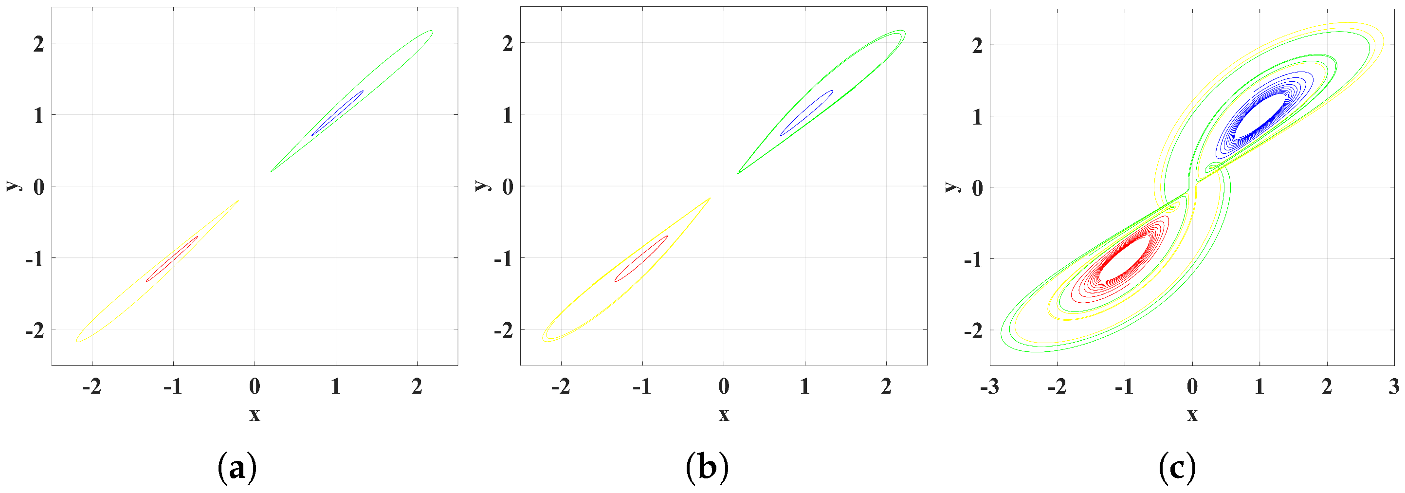
3.4. Coexistence of Attractors

The coexistence attractor is a complex dynamic feature, which means that the dissipative system uses the same set of parameters and appears in the same trajectory under different combinations of initial values. We decided to fix the parameters ( a , b , k , m , n ) = ( 1 , 0.01 , 5 , 0.1 , 0.01 ) and set four initial states from the x y plane direction of the attractor phase diagram. State 1: The initial values are ( 0.7 , 0.7 , 0.7 , 1 , 1 ) and the color is blue. State 2: The initial values are ( 0.7 , 0.7 , 0.7 , 1 , 1 ) and the color is red. State 3: The initial values are ( 0.2 , 0.2 , 0.2 , 0.1 , 0.1 ) and the color is green. State 4: The initial values are ( 0.2 , 0.2 , 0.2 , 0.1 , 0.1 ) and the color is yellow. The time range is 100. When c = 0.005 , the attractor shows that period-1 of State 1 and State 2 coexists with period-1 of State 3 and State 4, as shown in Figure 7a. When c = 0.017 , the attractor shows that period-1 of State 1 and State 2 coexists with the period-2 of State 3 and State 4, as shown in Figure 7b. When c = 0.2 , the attractor shows that the chaos of State 1 and State 2 coexists with the chaos of State 3 and State 4, as shown in Figure 7c.

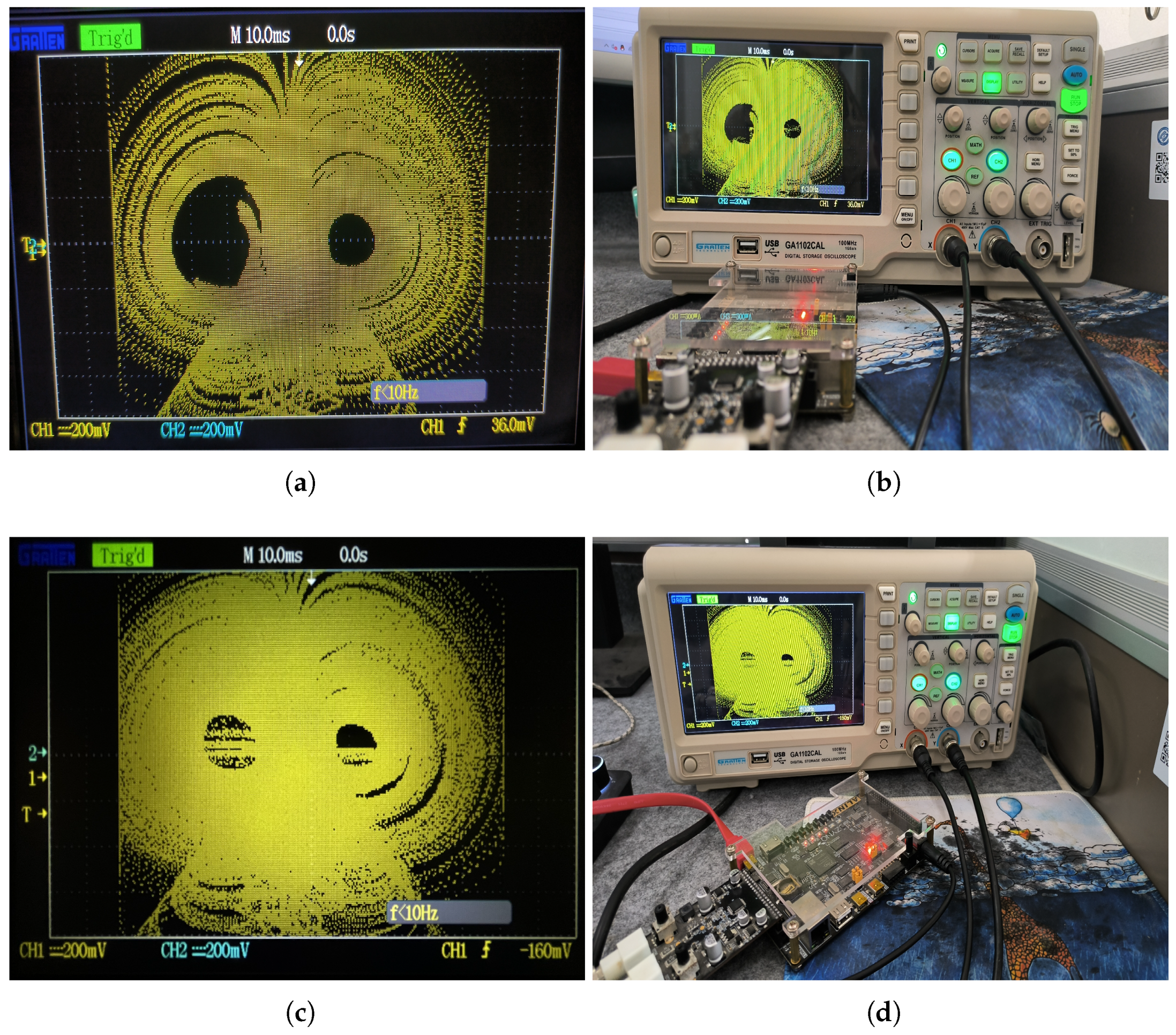
4. FPGA Implementation

Field programmable gate arrays (FPGA) are increasingly used for their high parallelism, customizability and reconfigurability, and the design and test cycle costs of FPGA chips are extremely low. Followed by discrete algorithm, we chose a universal fourth-order classical Runge–Kutta method (RK4) for discretization of continuous chaotic systems. The formula is as follows:
K 1 = Δ h ( x k , u k ) K 2 = Δ h ( x k + Δ h 2 , u k + K 1 2 ) K 3 = Δ h ( x k + Δ h 2 , u k + K 2 2 ) K 4 = Δ h ( x k + Δ h , u k + K 3 ) u k + 1 = u k + K 1 + 2 K 2 + 2 K 3 + K 4 6
We set the number of Δ h iteration steps to 0.001, and K 1 , K 2 , K 3 , K 4 represent the slope values of the four points in the interval [ x k , x k + 1 ] , respectively. During the iteration, u k provides data for the system and u k + 1 obtains data for the next iteration.
During the experiment, the development tool for the hardware implementation was Vivado 2018.3, and it is essential to note that the floating-point IP core provided by Vivado was used. Additionally, the development board for hardware implementation was AX7020, made by ALINX, and the FPGA chip was XC7Z0202CLG400I, made by Xilinx. The floating-point standard was IEEE754 with 32-bit precision, including 1 symbol bit, 8 exponent bits and 23 fraction bits. The simulation results on FPGA show the phase diagrams of the System (1) in the x z plane in Figure 8a. Figure 8c shows the phase diagrams of system (10) in the x z plane. Figure 8b shows the experimental apparatus of Figure 8a. Figure 8d shows the experimental apparatus of Figure 8c. According to these results, the FPGA experimental results agree with the MATLAB simulation results. This shows that the two systems are capable of discretization and have the potential to be applied in the field of network security communication.

5. Conclusions

In this paper, based on the classical Sprott-C system, we constructed a 4D hyperchaotic system (1) with seven terms as simply as in [58] under the coupling method of expanding the dimensions, adding nonlinear terms, introducing control parameters and controlling the range of values of b in order to avoid the phenomenon of rapid divergence. To refine system (1), a magnetically controlled memristor was introduced into the system, and the dimensionality was expanded to construct a 5D hidden attractor memristive hyperchaotic system. This makes the dynamical behavior of the system more complex, and there are multistability phenomena coexisting with periodic attractors and chaotic attractors, and the nonlinear motion is more complete. Finally, we designed the implementation of FPGA-based digital circuits for both systems, and the experimental results are consistent with the oscilloscope display, hardware experimental results and MATLAB simulations. In the future, we will apply the new system with innovations such as pseudo-random generators as a way to realize its value in secure communication and the biomedical field.

Author Contributions

Conceptualization, F.Y. and W.Z.; methodology, W.Z. and X.X.; software, W.Z. and W.Y.; validation, F.Y., W.Z. and S.C.; formal analysis, F.Y. and W.Z.; investigation, W.Z.; resources, F.Y. and S.C.; data curation, W.Z.; writing—original draft preparation, F.Y. and W.Z.; writing—review and editing, F.Y., W.Z. and C.W.; visualization, Y.L.; supervision, J.Z. and C.W.; project administration, F.Y. and W.Y.; funding acquisition, S.C. and J.Z. All authors have read and agreed to the published version of the manuscript.

Funding

This work was supported by the Natural Science Foundation of Hunan Province under Grants 2022JJ30624, 2022JJ10052 and 2021JJ30741; the Scientific Research Fund of Hunan Provincial Education Department under grant 21B0345; the National Natural Science Foundation of China under Grant 62172058; and the Postgraduate Training Innovation Base Construction Project of Hunan Province under Grant 2020-172-48.

Institutional Review Board Statement

Not applicable.

Informed Consent Statement

Not applicable.

Data Availability Statement

The data that support the findings of this study are available from the corresponding author upon reasonable request.

Acknowledgments

The authors thank the editors and reviewers for their hard work, who have made outstanding contributions to the improvement of the quality of this article!

Conflicts of Interest

The authors declare no conflict of interest.

References

  1. Wan, Q.; Yan, Z.; Li, F.; Chen, S.; Liu, J. Complex dynamics in a Hopfield neural network under electromagnetic induction and electromagnetic radiation. Chaos 2022, 32, 073107. [Google Scholar] [CrossRef] [PubMed]
  2. Shen, H.; Yu, F.; Kong, X.; Mokbel, A.A.M.; Wang, C.; Cai, S. Dynamics study on the effect of memristive autapse distribution on Hopfield neural network. Chaos 2022, 32, 083133. [Google Scholar] [CrossRef]
  3. Lin, H.; Wang, C.; Sun, Y.; Wang, T. Generating n-scroll chaotic attractors from a memristor-based magnetized hopfield neural network. IEEE Trans. Circuits Syst. II Express Briefs 2023, 70, 311–315. [Google Scholar] [CrossRef]
  4. Shen, H.; Yu, F.; Wang, C.; Sun, J.; Cai, S. Firing mechanism based on single memristive neuron and double memristive coupled neurons. Nonlinear Dyn. 2022, 110, 3807–3822. [Google Scholar] [CrossRef]
  5. Wen, Z.; Wang, C.; Deng, Q.; Lin, H. Regulating memristive neuronal dynamical properties via excitatory or inhibitory magnetic field coupling. Nonlinear Dyn. 2022, 110, 3823–3835. [Google Scholar] [CrossRef]
  6. Lu, Y.M.; Wang, C.H.; Deng, Q.L.; Xu, C. The dynamics of a memristor-based Rulkov neuron with the fractional-order difference. Chin. Phys. B 2022, 31, 060502. [Google Scholar] [CrossRef]
  7. Ma, M.; Lu, Y.; Li, Z.; Sun, Y.; Wang, C. Multistability and Phase Synchronization of Rulkov Neurons Coupled with a Locally Active Discrete Memristor. Fractal Fract. 2023, 7, 82. [Google Scholar] [CrossRef]
  8. Zhou, C.; Wang, C.; Yao, W.; Lin, H. Observer-based synchronization of memristive neural networks under DoSattacks and actuator saturation and its application to image encryption. Appl. Math. Comput. 2022, 425, 127080. [Google Scholar]
  9. Ma, M.; Xiong, K.; Li, Z.; Sun, Y. Dynamic Behavior Analysis and Synchronization of Memristor-Coupled Heterogeneous Discrete Neural Networks. Mathematics 2023, 11, 375. [Google Scholar] [CrossRef]
  10. Long, M.; Chen, Y.; Peng, F. Simple and accurate analysis of BER performance for DCSK chaotic communication. IEEE Commun. Lett. 2011, 15, 1175–1177. [Google Scholar] [CrossRef]
  11. Yu, F.; Yu, Q.; Chen, H.; Kong, X.; Mokbel, A.A.M.; Cai, S.; Du, S. Dynamic analysis and audio encryption application in IoT of a multi-scroll fractional-order memristive Hopfield neural network. Fractal Fract. 2022, 6, 370. [Google Scholar] [CrossRef]
  12. Lin, H.; Wang, C.; Cui, L.; Sun, Y.; Zhang, X.; Yao, W. Hyperchaotic memristive ring neural network and application in medical image encryption. Nonlinear Dyn. 2022, 110, 841–855. [Google Scholar] [CrossRef]
  13. Yu, F.; Shen, H.; Zhang, Z.; Huang, Y.; Cai, S.; Du, S. A new multi-scroll Chua’s circuit with composite hyperbolic tangent-cubic nonlinearity: Complex dynamics, Hardware implementation and Image encryption application. Integration 2021, 81, 71–83. [Google Scholar] [CrossRef]
  14. Li, X.; Zhou, L.; Tan, F. An image encryption scheme based on finite-time cluster synchronization of two-layer complex dynamic networks. Soft Comput. 2022, 26, 511–525. [Google Scholar] [CrossRef]
  15. Yu, F.; Kong, X.; Mokbel, A.A.M.; Yao, W.; Cai, S. Complex Dynamics, Hardware Implementation and Image Encryption Application of Multiscroll Memeristive Hopfield Neural Network with a Novel Local Active Memeristor. IEEE Trans. Circuits Syst. II Express Briefs 2022, 70, 326–330. [Google Scholar] [CrossRef]
  16. Korolj, A.; Wu, H.T.; Radisic, M. A healthy dose of chaos: Using fractal frameworks for engineering higher-fidelity biomedical systems. Biomaterials 2019, 219, 119363. [Google Scholar] [CrossRef]
  17. Lin, H.; Wang, C.; Cui, L.; Sun, Y.; Xu, C.; Yu, F. Brain-like initial-boosted hyperchaos and application in biomedical image encryption. IEEE Trans. Ind. Inform. 2022, 18, 8839–8850. [Google Scholar] [CrossRef]
  18. Yu, F.; Shen, H.; Yu, Q.; Kong, X.; Sharma, P.K.; Cai, S. Privacy Protection of Medical Data Based on Multi-Scroll Memristive Hopfield Neural Network. IEEE Trans. Netw. Sci. Eng. 2022, 1–14. [Google Scholar] [CrossRef]
  19. Deng, Z.; Wang, C.; Lin, H.; Sun, Y. A Memristive Spiking Neural Network Circuit with Selective Supervised Attention Algorithm. IEEE Trans. Comput. Aided Des. Integr. Circuits Syst. 2022. [Google Scholar] [CrossRef]
  20. Khennaoui, A.A.; Ouannas, A.; Momani, S.; Almatroud, O.A.; Al-Sawalha, M.M.; Boulaaras, S.M.; Pham, V.T. Special Fractional-Order Map and Its Realization. Mathematics 2022, 10, 4474. [Google Scholar] [CrossRef]
  21. Bao, H.; Hua, Z.; Liu, W.; Bao, B. Discrete memristive neuron model and its interspike interval-encoded application in image encryption. Sci. China Sci. 2021, 64, 2281–2291. [Google Scholar] [CrossRef]
  22. Yu, F.; Kong, X.; Chen, H.; Yu, Q.; Cai, S.; Huang, Y.; Du, S. A 6D fractional-order memristive hopfield neural network and its application in image encryption. Front. Phys. 2022, 10, 847385. [Google Scholar] [CrossRef]
  23. Azam, A.; Aqeel, M.; Sunny, D.A. Generation of Multidirectional Mirror Symmetric Multiscroll Chaotic Attractors (MSMCA) in Double Wing Satellite Chaotic System. Chaos Solitons Fractals 2022, 155, 111715. [Google Scholar] [CrossRef]
  24. Ai, W.; Sun, K.; Fu, Y. Design of multiwing-multiscroll grid compound chaotic system and its circuit implementation. Int. J. Mod. Phys. C 2018, 29, 1850049. [Google Scholar] [CrossRef]
  25. Yu, F.; Chen, H.; Kong, X.; Yu, Q.; Cai, S.; Huang, Y.; Du, S. Dynamic analysis and application in medical digital image watermarking of a new multi-scroll neural network with quartic nonlinear memristor. Eur. Phys. J. Plus 2022, 137, 434. [Google Scholar] [CrossRef]
  26. Sprott, J.C. Some simple chaotic flows. Phys. Rev. E 1994, 50, R647. [Google Scholar] [CrossRef]
  27. Wei, Z.; Yang, Q. Dynamical analysis of the generalized Sprott C system with only two stable equilibria. Nonlinear Dyn. 2012, 68, 543–554. [Google Scholar] [CrossRef]
  28. Wei, Z.; Moroz, I.; Liu, A. Degenerate Hopf bifurcations, hidden attractors, and control in the extended Sprott E system with only one stable equilibrium. Turk. J. Math. 2014, 38, 672–687. [Google Scholar] [CrossRef] [Green Version]
  29. Han, X.; Mou, J.; Jahanshahi, H.; Cao, Y.; Bu, F. A new set of hyperchaotic maps based on modulation and coupling. Eur. Phys. J. Plus 2022, 137, 523. [Google Scholar] [CrossRef]
  30. Li, X.; Mou, J.; Banerjee, S.; Wang, Z.; Cao, Y. Design and DSP implementation of a fractional-order detuned laser hyperchaotic circuit with applications in image encryption. Chaos Solitons Fractals 2022, 159, 112133. [Google Scholar] [CrossRef]
  31. Lai, Q.; Yang, L.; Liu, Y. Design and realization of discrete memristive hyperchaotic map with application in image encryption. Chaos Solitons Fractals 2022, 165, 112781. [Google Scholar] [CrossRef]
  32. Peng, Z.; Yu, W.; Wang, J.; Zhou, Z.; Chen, J.; Zhong, G. Secure communication based on microcontroller unit with a novel five-dimensional hyperchaotic system. Arab. J. Sci. Eng. 2022, 47, 813–828. [Google Scholar] [CrossRef]
  33. Yan, S.; Li, L.; Gu, B.; Cui, Y.; Wang, J.; Song, J. Design of hyperchaotic system based on multi-scroll and its encryption algorithm in color image. Integration 2023, 88, 203–221. [Google Scholar] [CrossRef]
  34. Goufo, E.F.D. Linear and rotational fractal design for multiwing hyperchaotic systems with triangle and square shapes. Chaos Solitons Fractals 2022, 161, 112283. [Google Scholar] [CrossRef]
  35. Al-hayali, M.A.; Al-Azzawi, F.S. A 4D hyperchaotic Sprott S system with multistability and hidden attractors. J. Phys. Conf. Ser. 2021, 1879, 032031. [Google Scholar] [CrossRef]
  36. Ojoniyi, O.S.; Njah, A.N. A 5D hyperchaotic Sprott B system with coexisting hidden attractors. Chaos Solitons Fractals 2016, 87, 172–181. [Google Scholar] [CrossRef]
  37. Lin, H.; Wang, C.; Xu, C.; Zhang, X.; Iu, H.H. A memristive synapse control method to generate diversified multi-structure chaotic attractors. IEEE Trans. Comput. Aided Des. Integr. Circuits Syst. 2022. [Google Scholar] [CrossRef]
  38. Wan, Q.; Yan, Z.; Li, F.; Liu, J.; Chen, S. Multistable dynamics in a Hopfield neural network under electromagnetic radiation and dual bias currents. Nonlinear Dyn. 2022, 109, 2085–2101. [Google Scholar] [CrossRef]
  39. Ramadoss, J.; Almatroud, O.A.; Momani, S.; Pham, V.T.; Thoai, V.P. Discrete memristance and nonlinear term for designing memristive maps. Symmetry 2022, 14, 2110. [Google Scholar] [CrossRef]
  40. Ma, M.; Yang, Y.; Qiu, Z.; Peng, Y.; Sun, Y.; Li, Z.; Wang, M. A locally active discrete memristor model and its application in a hyperchaotic map. Nonlinear Dyn. 2022, 107, 2935–2949. [Google Scholar] [CrossRef]
  41. Ramadoss, J.; Ouannas, A.; Tamba, V.K.; Grassi, G.; Momani, S.; Pham, V.T. Constructing non-fixed-point maps with memristors. Eur. Phys. J. Plus 2022, 137, 211. [Google Scholar] [CrossRef]
  42. Yu, F.; Qian, S.; Chen, X.; Huang, Y.; Liu, L.; Shi, C.; Cai, S.; Song, Y.; Wang, C. A new 4D four-wing memristive hyperchaotic system: Dynamical analysis, electronic circuit design, shape synchronization and secure communication. Int. J. Bifurc. Chaos 2020, 30, 2050147. [Google Scholar] [CrossRef]
  43. Kamdem Kuate, P.D.; Lai, Q.; Fotsin, H. Complex behaviors in a new 4D memristive hyperchaotic system without equilibrium and its microcontroller-based implementation. Eur. Phys. J. Spec. Top. 2019, 228, 2171–2184. [Google Scholar] [CrossRef]
  44. Yu, F.; Xu, S.; Xiao, X.; Yao, W.; Huang, Y.; Cai, S.; Yin, B.; Li, Y. Dynamics analysis, FPGA realization and image encryption application of a 5D memristive exponential hyperchaotic system. Integration 2023, 90, 58–70. [Google Scholar] [CrossRef]
  45. Yu, F.; Liu, L.; Qian, S.; Li, L.; Huang, Y.; Shi, C.; Cai, S.; Wu, X.; Du, S.; Wan, Q. Chaos-based application of a novel multistable 5D memristive hyperchaotic system with coexisting multiple attractors. Complexity 2020, 2020, 8034196. [Google Scholar] [CrossRef] [Green Version]
  46. Ramamoorthy, R.; Rajagopal, K.; Leutcho, G.D.; Krejcar, O.; Namazi, H.; Hussain, I. Multistable dynamics and control of a new 4D memristive chaotic Sprott B system. Chaos Solitons Fractals 2022, 156, 111834. [Google Scholar] [CrossRef]
  47. Koyuncu, İ.; Tuna, M.; Pehlivan, İ.; Fidan, C.B.; Alçın, M. Design, FPGA implementation and statistical analysis of chaos-ring based dual entropy core true random number generator. Analog Integr. Circuits Signal Process. 2020, 102, 445–456. [Google Scholar] [CrossRef]
  48. Ding, S.; Wang, N.; Bao, H.; Chen, B.; Wu, H.; Xu, Q. Memristor synapse-coupled piecewise-linear simplified Hopfield neural network: Dynamics analysis and circuit implementation. Chaos Solitons Fractals 2023, 166, 112899. [Google Scholar] [CrossRef]
  49. Yu, F.; Zhang, Z.; Shen, H.; Huang, Y.; Cai, S.; Jin, J.; Du, S. Design and FPGA implementation of a pseudo-random number generator based on a Hopfield neural network under electromagnetic radiation. Front. Phys. 2021, 9, 690651. [Google Scholar] [CrossRef]
  50. Chen, H.; He, S.; Pano Azucena, A.D.; Yousefpour, A.; Jahanshahi, H.; López, M.A.; Alcaraz, R. A multistable chaotic jerk system with coexisting and hidden attractors: Dynamical and complexity analysis, FPGA-based realization, and chaos stabilization using a robust controller. Symmetry 2020, 12, 569. [Google Scholar] [CrossRef] [Green Version]
  51. Shah, D.K.; Chaurasiya, R.B.; Vyawahare, V.A.; Pichhode, K.; Patil, M.D. FPGA implementation of fractional-order chaotic systems. AEU-Int. J. Electron. Commun. 2017, 78, 245–257. [Google Scholar] [CrossRef]
  52. Koyuncu, I.; Ozcerit, A.T.; Pehlivan, I. Implementation of FPGA-based real time novel chaotic oscillator. Nonlinear Dyn. 2014, 77, 49–59. [Google Scholar] [CrossRef]
  53. Mohamed, S.M.; Sayed, W.S.; Said, L.A.; Radwan, A.G. Reconfigurable fpga realization of fractional-order chaotic systems. IEEE Access 2021, 9, 89376–89389. [Google Scholar] [CrossRef]
  54. Sambas, A.; Vaidyanathan, S.; Zhang, X.; Koyuncu, I.; Bonny, T.; Tuna, M.; Alçin, M.; Zhang, S.; Sulaiman, I.M.; Awwal, A.M.; et al. A novel 3D chaotic system with line equilibrium: Multistability, integral sliding mode control, electronic circuit, FPGA implementation and its image encryption. IEEE Access 2022, 10, 68057–68074. [Google Scholar] [CrossRef]
  55. Lai, Q.; Wang, Z.; Kuate, P.D.K. Dynamical analysis, FPGA implementation and synchronization for secure communication of new chaotic system with hidden and coexisting attractors. Mod. Phys. Lett. B 2022, 36, 2150538. [Google Scholar] [CrossRef]
  56. Chen, W.; Jin, J.; Chen, C.; Yu, F.; Wang, C. A Disturbance Suppression Zeroing Neural Network for Robust Synchronization of Chaotic Systems and Its FPGA Implementation. Int. J. Bifurc. Chaos 2022, 32, 2250210. [Google Scholar] [CrossRef]
  57. Yu, F.; Zhang, Z.; Shen, H.; Huang, Y.; Cai, S.; Du, S. FPGA implementation and image encryption application of a new PRNG based on a memristive Hopfield neural network with a special activation gradient. Chin. Phys. B 2022, 31, 020505. [Google Scholar] [CrossRef]
  58. Sheet, A.T.; Al-Azzawi, S.F. A New Simple 4D Hyperchaotic Sprott-B System with Seven-Terms. In Proceedings of the 2022 International Conference on Computer Science and Software Engineering (CSASE), Duhok, Iraq, 15–17 March 2022; pp. 65–70. [Google Scholar]
Figure 1. Ref. [58] System attractor dispersion diagram under initial conditions ( 0.3 , 0.2 , 0.3 , 0.1 ) , and phase diagrams of system (1) under initial conditions ( 0.3 , 0.2 , 0.3 , 0.1 ) . (a) Ref. [58] System attractor diagram with ( a , b ) = ( 0.1 , 0.09 ) in x u plane, (b) System (1) attractor diagram with ( a , b ) = ( 0.1 , 0.1 ) in x y plane, (c) System (1) attractor diagram with ( a , b ) = ( 0.1 , 0.1 ) in x z plane, (d) System (1) attractor diagram with ( a , b ) = ( 0.1 , 0.1 ) in x y z plane.
Mathematics 11 00701 g001
Figure 2. Lyapunov exponent and phase diagram of system (1) with ( a , b ) = ( 1 , 0.001 ) under initial conditions ( 1 , 1 , 1 , 1 ) . (a) Lyapunov exponent of system (1). (b) Phase diagram of system (1) in x u plane.
Mathematics 11 00701 g002
Figure 3. Bifurcation diagram of system (1) with initial conditions ( 0.1 , 0.1 , 0.1 , 0.1 ) . (a) Bifurcation diagram of a with b = 0.1 . (b) Bifurcation diagram of b with a = 0.1 .
Mathematics 11 00701 g003
Figure 4. Lyapunov exponent spectra of System 1 with different initial conditions. (a) Lyapunov exponent spectrum with a [ 0 , 10 ] and b = 0.01 under I C = ( 0.1 , 0.1 , 0.1 , 0.1 ) . (b) Lyapunov exponent spectrum with b [ 10 , 0 ] and a = 0.1 under I C = ( 0.1 , 0.1 , 0.1 , 0.1 ) . (c) Lyapunov exponent spectrum with a [ 0 , 10 ] and b = 0.01 under I C = ( 1 , 1 , 1 , 1 ) . (d) Lyapunov exponent spectrum with b [ 10 , 0 ] and a = 0.1 under I C = ( 1 , 1 , 1 , 1 ) .
Mathematics 11 00701 g004
Figure 5. System (10) attractor phase diagram with ( a , b , c , k , m , n ) = ( 2 , 0.01 , 0.5 , 5 , 0.1 , 0.01 ) under initial conditions ( 1 , 1 , 1 , 1 , 1 ) . (a) System (10), x y plane. (b) System (10), x z plane. (c) System (10), x y z plane.
Mathematics 11 00701 g005
Figure 6. Phase diagrams with different c; Lyapunov exponent spectrum and the bifurcation diagram at c ( 0 , 0.5 ] . (a) Period-1 attractor with c = 0.01 ; (b) chaotic attractor, c = 0.12 ; (c) hyperchaotic attractor, c = 0.5 ; (d) Lyapunov exponent spectrum with c ( 0 , 0.5 ] ; (e) bifurcation diagram, c ( 0 , 0.5 ] .
Mathematics 11 00701 g006
Figure 7. Coexistence of attractors with ( a , b , k , m , n ) = ( 1 , 0.01 , 5 , 0.1 , 0.01 ) under initial conditions ( 0.7 , 0.7 , 0.7 , 1 , 1 ) , ( 0.7 , 0.7 , 0.7 , 1 , 1 ) , ( 0.2 , 0.2 , 0.2 , 0.1 , 0.1 ) and ( 0.2 , 0.2 , 0.2 , 0.1 , 0.1 ) . (a) c = 0.005 , period-1 of State 1 and State 2 coexists with period-1 of State 3 and State 4. (b) c = 0.017 , period-1 of State 1 and State 2 coexists with the chaos of State 3 and State 4. (c) c = 0.2 , chaos of State 1 and State 2 coexists with the chaos of State 3 and State 4.
Mathematics 11 00701 g007
Figure 8. Oscilloscope experiment results. (a) System (1) phase diagram of the x z plane by the FPGA. (b) The experimental apparatus of Figure 8a. (c) System (10) phase diagram of the x z plane by the FPGA. (d) The experimental apparatus of Figure 8c.
Mathematics 11 00701 g008
Disclaimer/Publisher’s Note: The statements, opinions and data contained in all publications are solely those of the individual author(s) and contributor(s) and not of MDPI and/or the editor(s). MDPI and/or the editor(s) disclaim responsibility for any injury to people or property resulting from any ideas, methods, instructions or products referred to in the content.

