Article

Are State-Owned Enterprises Really Ineffective? An Empirical Study Based on Stochastic Frontier Analysis

1
School of Business, Shandong University, Weihai 264209, China
2
School of Culture and Communication, Shandong University, Weihai 264209, China
*
Author to whom correspondence should be addressed.
Mathematics 2023, 11(3), 657; https://doi.org/10.3390/math11030657
Submission received: 20 November 2022 / Revised: 7 January 2023 / Accepted: 18 January 2023 / Published: 28 January 2023

Abstract

:
Technical efficiency (TE) and total factor productivity (TFP) are important criteria to ensure the enhancement of the quality and efficiency of state-owned enterprises (SOEs) and function as important indicators to assess the quality of their accomplishments. The purpose of this study is to explore whether the efficiency of SOEs is higher or lower than that of private enterprises. Transcendental logarithmic production function and stochastic frontier analysis (SFA) are used to assess the TE and TFP of listed central SOEs, local SOEs, and private enterprises, the data of which were taken from 2006–2020. The results show that the sampled private enterprises had the highest average TE during the study period, followed by the central and local SOEs. The private enterprises also had the highest average TFP growth rate, followed by the local and central SOEs. The TFP decompositions show that the TE change (TEC) and technical change (TC) indices of the SOEs were lower than those of the private enterprises. The TC, TEC, and scale change (SC) are limiting the TFP growth rates of the SOEs in labor-intensive industries. The SC of the SOEs has changed less than that of private enterprises in the sampled capital-intensive industries. Northern and southern China had the highest rates of TE and TFP growth. Indeed, this paper measures and decomposes TFP, and analyzes the efficiency of SOEs and private enterprises in different industries and regions in an international context.
Keywords:
SOEs; efficiency; SFA
MSC:
91B38

1. Introduction

As the goal of economic development begins to shift from the pursuit of quantity to quality, total factor productivity (TFP) has gradually replaced factor inputs to become the main driving force for economic growth [1]. According to the report of the Chinese Communist Party’s 19th National Congress, China’s economy has changed from a stage of high-speed growth to one of high-quality development, which is critical to the enhancement of reforms in economic development and TFP. North [2], the father of new institutional economics, suggested that an effective property rights system may provide personal incentives, which are key determinants of economic growth and production efficiency [3].
State-owned enterprises (SOEs) are an important means for China’s central and local governments to directly participate in the market. Compared with private enterprises, SOEs also undertake various social functions, such as stable employment. Many differences exist between SOEs and private enterprises in terms of how they obtain resources and in the factor prices they receive. This mechanism hinders the free flow of production factors to a certain extent, resulting in resource misallocation among regions, industries, and enterprises [4,5]. As the economy’s main driver, SOEs are not only an important basis for the socialist market economy with Chinese characteristics, but also an important pillar for furthering the country’s modernization and defending the people’s common interests. According to China’s 14th Five-Year Plan for National Economic and Social Development, extensions to the reforming of the SOEs should be guided by the need to increase efficiency [6]. According to the report of the 19th National Congress, China will adhere to the principles of quality and efficiency first; efforts will be made to prioritize supply-side structural reforms, increase TFP, and promote high-quality economic development, efficiency, and power [7]. The report repeatedly mentions TFP and emphasizes that it could be decomposed into efficiency and dynamic changes. Hence, the study of the TFP of SOEs from a microeconomic viewpoint is of strategic importance.
In the face of increasingly high costs of China’s factor resources, the efficiency of industrial enterprises will directly affect the quality and speed of economic growth. The purpose of this study is to explore whether SOEs are more or less efficient than private enterprises. The research objectives of this paper are to (1) measure the overall efficiency of industrial enterprises with different ownership structures and (2) compare the efficiency differences of enterprises with different ownership structures by regions and industries. The research in this paper is of great reference value for objective evaluations of the performance of past industrial policies and formulations of new policies and plans.
Using micro-level data of enterprises and a stochastic frontier production model, this study investigates the trends of the TFP and growth factor decomposition of listed central SEOs, local SEOs, and private enterprises by using data from 2007 to 2020. The profit of the enterprise group, which was the subject of this study, accounted for 51.56% of China’s gross national product in 2020. Therefore, the empirical results are of great significance to in-depth analyses of the development trend and potential of China’s industrial productivity.
A long history of academic debate on the efficiency of SOEs has produced a large number of theoretical and empirical studies, many of which were conducted on the transitional economies of eastern Europe, countries of the former Soviet Union, and Brazil [8,9,10,11]. The debate on the efficiency of Chinese SOEs [4,12] has resulted in the formation of two main opposing viewpoints: SOEs are usually inefficient vs. efficient. Section 2 discusses the literature on Chinese SOEs.
Evaluations of the effects of reforming SOEs have always been contentious in academic circles and their production efficiency has been one of the main topics of interest. Are SOEs usually inefficient? Do they really have lower production efficiency than other types of businesses? Methods of measuring TFP include the Solow residual method, stochastic frontier analysis (SFA), data envelopment analysis (DEA), and index analysis [13]. The first two are parametric methods, whereas the latter two are nonparametric, which mainly use linear programming to determine the production frontiers and measure TE without setting the frontier functions or estimating the parameters in advance. Additionally, the latter methods do not consider the influences of random factors on production efficiency; the stability of their calculations is low, and the parameters cannot be statistically tested. The Solow residual method attributes all the parts, except the contributions of factor inputs, of output growth to technological progress, thereby implying that all producers could achieve optimal production efficiency, which is difficult to achieve in actual production. Therefore, large errors are often present in the estimation of TFP. As a parametric method, the SFA can separate the inefficiency term from the random error term to consider the influences of random factors; thus, the measurement results would be closer to reality [14]. The non-parametric method of DEA to measure TFP [15,16], as well as the Solow residual method to measure the TFP of China’s manufacturing industry and Shanghai, respectively [17,18], have been reported in the literature. In this paper, the stochastic frontier method is used to consider the influence of stochastic factors on the production process; the disadvantages of the nonparametric method and Solow residual method are avoided. In addition, the SFA in this paper is based on the transcendental logarithmic production function. Compared with the Cobb Douglas function, the proposed method reduces the restrictions on the invariability of returns to scale and elasticity of substitution, is more consistent with production behavior and has more flexible parameters. The stochastic frontier method can also consider the interaction of input factors and time trend. This is the first novel aspect of this paper, compared to other papers published in this field of study.
Initially proposed by Aigner, Lover, and Schmidt [19], and Meeusen, Van den Broeck [20], the stochastic frontier production model soon became a remarkable branch of econometrics. The model assumes that enterprises cannot reach the best level of cutting-edge technology because of the loss of efficiency in the production process caused by non-price factors, such as organization, management, and system.
The scope of the stochastic frontier function is broad and it can be applied to diverse fields, such as agriculture [21,22], manufacturing [23], commercial banking [14,24,25], cultural industry [26], tax collection and management [27], open-end funds [28], insurance [29], services [30,31,32], research and development [33], innovation efficiency [34,35,36,37], urbanization [38], electric power industry [39], energy efficiency [40,41,42,43,44], and energy savings and emission reduction [45]. However, few studies have been conducted on the measurements of the TFP or TE of listed companies. In particular, most studies have only measured TFP without decomposition [17]. Even studies that have decomposed TFP have only done so for short time spans [46]. Hence, both types of studies have not fully reflected the levels and changing trends of TE. How can the TE of SOEs be effectively measured? To what extent do the sub-indicators of TFP affect the efficiency of SOEs? These questions have important theoretical and practical significance for the reform of China’s SOEs, industrial development planning, and innovation. This is another novel aspect of this paper, compared to other papers published in this field of study.
Using the transcendental logarithmic production function and SFA to measure the technical efficiency (TE) and TFP, as well as their decompositions, of all listed central SOEs, local SOEs, and private enterprises in various industries and regions for 2006 to 2020, we have examined if SOEs are more or less efficient than other types of businesses and what are the variations in key efficiency criteria and disparities among the efficiency of different industries. This paper makes three contributions to the literature. First, our investigation into the influence of company ownership structure on efficiency contributes marginally to the thesis that the property rights system is a critical determinant of economic growth. Second, we use data from 2006 to 2020 of all the listed companies and have updated the time range of our study to provide an up-to-date explanation of the effects of corporate ownership on efficiency. Third, we investigated the decompositions of the enterprises’ TE and TFP and examined the effect mechanism of their varying levels of efficiency in terms of ownership structure, region, and industry. This empirical study on the differences between the efficiency of SOEs and private enterprises provides a reference for the governance model of the coexistence and co-development of SOEs and private enterprises under mixed ownership, which is conducive to the formation of a positive cycle of coordination between both types of enterprises.
The remainder of this paper is structured as follows: Section 2 reviews the literature, Section 3 proposes the SFA and the decomposition framework of the TFP growth rate, Section 4 presents the overall measurements of TE, Section 5 discusses a comparative analysis of the TFP growth rate decomposition, and Section 6 presents the conclusions and relevant policy recommendations.

2. Literature Review

2.1. The Theory of SOE Inefficiency

Estrin et al. [9] argued that most studies in China had found that the effects of non-state ownership on TFP were usually positive but sometimes negligible or negative. Zheng et al. [47] suggested that SOEs were less productive, but they survived because of better access to credit markets. Using data from 2002 to 2009, Hao et al. [48] applied a comprehensive factor evaluation method and concluded that the operational efficiency of private enterprises was higher than that of SOEs. Fan et al. [49] used the DEA method and concluded that the overall efficiency and TE of Chinese SOEs are lower than those of foreign and private firms. Xu [50] used a stochastic frontier approach to measure the productivity losses of listed companies for 2006–2015; the study concluded that SOEs had higher efficiency losses than did private enterprises. Berkowitz et al. [51] concluded that the productivity of Chinese SOEs increased as a result of the policy of “manage large enterprises well but ease control over smaller ones”, but the SEOs still lagged behind foreign and private firms. Zhang et al. [52] used a three-stage DEA model to study the productive efficiency of manufacturing firms for 2009–2014 and concluded that the overall efficiency and pure TE of SOEs were lower than those of private firms. By calculating TFP at the firm level in the mining and manufacturing sectors, Li and Yang [53] found that SOEs had higher loss rates and lower TFP. Based on a firm productivity perspective, Wang Wanjun and Liu [54] found that the proportion of zombie firms among SOEs were much higher than the proportion of private firms. Using data from the China Industrial Enterprise Database, Yin et al. [55] showed that enterprises with mixed ownership were more efficient than SOEs and that a diversified ownership structure was conducive to enterprise efficiency. Liu et al. [56] suggested that the average productivity of SOEs was lower than that of private enterprises.

2.2. The Theory of SOE Efficiency

Hao et al. [48] argued that SOEs undertook more social functions and had higher dynamic functional efficiency than did the other types of enterprises. Weighting and summing operational and functional efficiencies to obtain the total governance efficiency index for different types of enterprises showed that the overall trend of governance efficiency was higher for state-controlled enterprises and wholly controlled SOEs than for private enterprises. Using SFA and spatial econometric models, Zhao [57] concluded that SOEs were the center of technology diffusion and more efficient than private and foreign enterprises in promoting regional innovation efficiency spillover. Zhao and Fang [58] used the DEA method to calculate the mean value (0.613) of the combined innovation efficiency of SOEs for 2008–2015 and found that it was higher than that of non-SOEs (0.373). Tan et al. [59] studied the efficiency of commercial banks in countries along the 21st Century Maritime Silk Road and concluded that state-owned commercial banks were more efficient than non-state-owned commercial banks. Using the deviation between the actual and expected value of unit employment to measure labor investment efficiency, Kong Dongmin et al. [60] concluded that SOEs had higher labor investment efficiency than did private enterprises.
Using different methodologies to analyze the productivity of Chinese SOEs and private enterprises, these studies have drawn some significant conclusions but have remained limited to comparative analyses between a purely TFP perspective and the industry level. This study is innovative for the following reasons: first, the annual productivity of each range of firms was measured from a micro-firm perspective. Second, we applied SFA to decompose the growth rate of TFP.

3. Measurements and Decomposition

TFP refers to other factors that contribute to economic growth after the inputs of capital and labor factors have been removed. TFP has a more comprehensive response to whether the efficiency of input factors or the effects of technological progress on output has improved. This indicator can better reflect the comprehensive level and fluctuation of productivity than can single factor productivity. Three universal schemes can be used to measure the TFP of enterprises: total parameter estimation (SFA), semi-parameter estimation (LP [61] and OP [62]), and non-parameter estimation (DEA). OP can handle simultaneity bias and sample selection bias, but other problems may be present. For example, the investment amounts of enterprises may be affected by the external environment and may not completely reflect the unobservable productivity, so the estimation may fail to meet the consistency condition. Because of the adjustment cost, the investments may not fully respond to the change in productivity levels, so a correlation between the regression quantity and the residual term would still be present, while the cost of adjusting the intermediate input is lower. LP can respond to the whole productivity term but uses intermediate inputs, so LP is not significantly better than OP, which uses investment as a proxy variable. Moreover, the Chinese economy is undergoing institutional transitions internally and is being influenced by international economics externally. As such, avoiding the many random disturbances and substantial factors that occur during economic growth is almost impossible. Therefore, DEA with deterministic boundaries may not be suitable for the measurement of the productivity of Chinese enterprises, whereas SFA will be relatively more reliable [63]. Therefore, we applied SFA to measure the productivity of listed central SOEs, local SOEs, and private enterprises by using the data from 2006 to 2020, then conducted a comparative analysis by industry, sub-industry, region, sub-region, and type of enterprise ownership.

3.1. Stochastic Frontier Production Model

An SFA model can be described by Equation (1):
Y i = f x i , β e v i u i   ( i = 1 ,   2 ,   ,   N ) ,
where Yi is the output, xi is the input, and β is the model parameter. The random disturbance εi is divided into two parts: vi to represent the statistical or random error term, and ui to express technical inefficiency or the non-negative error term.
The random error term v i ~ N ( 0 , σ v 2 ) is mainly caused by uncontrollable factors, such as natural disasters and weather. The non-negative error term u i ~ N + ( 0 , σ v 2 ) takes the truncated normal distribution (the part less than 0 is removed); ui and vi are independent of each other and the independent variables.
The model improved by Battese and Coelli [64] is widely used:
ln Y i t = β 0 + β j l n x i t + v i t u i t   ( i = 1 ,   2 ,   ,   N ;   t = 1 ,   2 ,   ,   T ) ,
where Yit and xit are the total output and input, respectively, of decision-making unit i in period t; β is a model parameter, v i t   is a random error term, uit = ui eη(t−T) is a non-negative error term, and η is an estimated parameter.
The efficiency level of enterprise i in period t is expressed by TEit = euit. If ui = 0, then TEit = 1, which indicates that the enterprise is in a state of TE. Otherwise, if u i t > 0 , then 0 < TEit < 1, which means a state of technical inefficiency exists. γ = σ u 2 σ u 2 + σ v 2 is used to judge if SFA should be used: when γ = 0, then σ v 2 = 0 , i.e., the random error term in Equation (2) is composed only of vit, so the least square method can be directly used for regression. When γ > 0, SFA should be adopted; TEit is mainly used to measure the distance between an enterprise’s output and the maximum output frontier under the condition of equal factor inputs. The greater the distance is, the lower is the TE.

3.2. Decomposition of TFP Growth Rate

Based on the analytical approach proposed by Kunbhakar [65] and used by Tu and Xiao [66], we decomposed the growth of TFP into contributions from four sources: (1) changes in TE (TEC), (2) efficiency of technological changes (TC), (3) changes in scale effects (SC), and (4) changes in factor allocation efficiency, (AE). The aim was to acquire a more comprehensive view for analyzing the structure of the components of the enterprises’ TFP growth rate.
The component of productivity change comes from the decisive part of the production frontier described by Equation in Section 3.1, combined with the general formula of productivity change, which is the Divisia index:
g T F P = y ˙ s k K ˙ s L L ˙
where the point on the variable represents the change rate of the variable, gTFP indicates the change rate of the TFP growth rate, and sk and sL, respectively, mean the shares of capital and labor in the total output;   S K = P K K P K K + P L K and S L = P L L P K K + P L L , where pK and pL represent the prices of capital and labor, respectively.
From the basic stochastic frontier production model y i t = f t , L i t , K i t ; β e v i t u i t , the partial derivative of the time variable t with respect to y can be obtained:
y ˙ = ln f t , L , K ; β t + ( ε K K ˙ + ε L L ˙ ) u t
where εK and εL are the output elasticities of the capital and labor, respectively. Equation (4) implies that the overall change in productivity is influenced by technological progress, changes in input factors, or changes in TE.
Substituting Equation (4) into Equation (3), we obtain:
g T F P = ln f t , L , K ; β t + RTS 1 λ K K ˙ + λ L L ˙ + λ K s K K ˙ + λ L s L L ˙   u t
where RTS = ε K + ε L represents the returns to scale, and λ K = ε K R T S and λ L = ε L R T S respectively represent the shares of labor and capital in the standardized output. Equation (5) divides the growth of TFP into four components listed below. The results show that the dual factors of technological progress and TE promote the growth of TFP, while the returns to scale measure the change in TFP caused by SC. In addition, ( λ K S K ) K ˙ + ( λ L S L ) L ˙ explains the inefficiency of factor allocation caused by the deviations of input factor prices in terms of the marginal product values of the factors.
The four components are thus defined:
(1)
TEC: u t ;
(2)
TC: ln f t , L , K ; β t ;
(3)
SC: RTS 1 λ K K ˙ + λ L L ˙ ;
(4)
AE: λ K s K K ˙ + λ L s L L ˙ .
TC refers to the increase in the maximum output that can be obtained from a given input level, thus capturing the upward transformation of the production function. TEC refers to the ability of an enterprise to obtain the maximum output at a given input level and can also measure the change in TFP due to the shift to the production function. SC refers to the change in TFP caused by the change in business scale, the influence of which depends on technology and factor accumulation. When the returns to scale (RTS) are constant (RTS = 1), SC is offset. With the increasing RTS (RTS > 1) and number of production factors, the productivity growth rate of the enterprises is higher. If the number of production factors decreases, the productivity change rate will also decrease. AE is the change in an enterprise’s ability to choose its input level and ensure that the input-price ratio is equal to the corresponding marginal output ratio; λ L + λ K = 1 , λ K S K , and λ L S L are symmetrical and opposite in sign. Therefore, the redistribution of factors, i.e., increasing labor intensity and decreasing capital investment, will inevitably change the allocation efficiency.
SC, TC, and TE are related to the technical part of TFP change, which can be calculated by estimated production technology (such as the output distance function and the parameters estimated by TE in Equation (1)). AE is caused by profit maximization, which violates the first-order condition. If there are some imperfections in the market (such as transaction costs, risks, quantity restrictions, incomplete information, or profits) or the assumption of implied profit maximization is not enough, a violation may occur. Because these influences are caused by market or behavioral conditions (they represent a part of technically undetermined TFP changes), AE is called the market part of TFP change and is the difference between the Divisia index and the three technical components: AE = gTFP − (SC + TC + TE).

4. Estimation and Decomposition of TFP of Chinese Listed Companies

4.1. Model Specifications

This study selected the transcendental logarithmic production function to construct the model, which has the advantages of flexible function form, strong tolerance, and easy estimation. Most importantly, compared with the Cobb–Douglas production function, the proposed function can effectively avoid the constant scale return and substitution elasticity between factors of C–D production function, and is more consistent with most production behaviors. The proposed production function is a second-order flexible function with adequate parameters, which can comprehensively reflect the impact of various input factors, technical change (TC) and the interaction between input factors and TC on the production frontier. In short, this function has certain research advantages. We set the parameter model as follows:
ln y i t = β 0 + β t t + β K ln K i t + β L ln L i t + 1 2 β t t · t 2 + 1 2 β K K · ln K i t 2 + 1 2 β L L · ln L i t 2 + 1 2 β K L · ln K i t · ln L i t                             + β K t ln K i t · t + β L t ln L i t · t + v i t u i t
where t signifies time trends, while lnyit, lnKit, and lnLit represent the logarithms of output, capital, and labor, respectively, of listed company i (i = 1, 2, …, N; t = 1, 2, …, 10) in year t; β indicates the parameter to be estimated; vit − uit is a composite random disturbance (εit); vit represents random error, reflecting the non-efficiency of the system, and uit represents technical loss error, reflecting technical inefficiency.
We adopted panel data. After considering the change path of efficiency, we chose the truncated normal distribution, which is a form of joint distribution.

4.2. Variables and Data

The data in this study are from the Wind and CSMAR databases for 2006 to 2020. Our research objects are 500 listed central SEOs, local SEOs, and private enterprises. When calculating enterprise efficiency, capital and output were subtracted from the 2006 data points to eliminate the influences of price factors. Moreover, we removed the financial sector and enterprise data for the years when capital and output were negative. All the original data were taken from the annual reports and consolidated financial statements of the listed enterprises and processed as follows: the output variable is industrial added value = depreciation of fixed assets + remuneration for workers + net production tax + earned surplus. The data on remuneration for workers came from “the compensation of employees’ payables”; the data on earned surplus came from “operating profit”, and the data on net production tax came from taxes and additional expenses. To eliminate the influences of price factors, the producer price index (PPI) (based on 2006) was used to subtract the output data. The capital input variable should be measured by the capital stock of each listed company, but the data on the capital stock were not provided in the statistical yearbooks. Therefore, we used the net value of fixed assets and fixed asset investment price index, based on 2006, for the reduction. Both indices were obtained from the China Statistical Yearbook 2020 [67]. The labor input variable should be measured by the labor time of standard labor intensity, but the statistical yearbooks lacked detailed labor data. Scholars usually substitute the number of employees for labor input, a method that we also adopted.
The decomposition involves calculating the cost shares of the input factors. To ensure the availability of data, this study followed Tu and Xiao [66] by adopting the current year sum of depreciation, amortization, and interest expenses as the costs of the capital inputs. Moreover, we used the compensation of employees’ payables as the labor input costs. The descriptive statistics of the indicators of the three types of listed companies are shown in Table 1.

4.3. Industry Classification Method

According to Lu Tong and Dang Yin [68] and the industry classification of the China Securities and Regulatory Commission (CSRC) 2012 [69], the manufacturing industry can be subdivided into 44 sub-industries classified into labor-, capital-, and technology-intensive, as shown in Table 2.
The term ‘labor-intensive industries’ refers to production that mainly depends on labor and the wage expenditures of which account for a large proportion of the production costs. These industries can be classified into 16 subsectors, such as mining, processing of agricultural products, and textiles, etc. Capital-intensive industries mainly rely on large amounts of capital input and belong to traditional state-owned monopoly industries. During China’s economic reforms and liberalization, private and foreign capital were introduced to improve the supply capacity and the enthusiasm of enterprises to operate independently. However, monopoly power still exists, because the nature of China’s society cannot achieve complete market competition. Capital-intensive industries include paper manufacturing, smelting and pressing of ferrous metals, transportation, warehousing, and postal services, among 18 other sub-industries. Technology-intensive industries are characterized by high investments, high risks, high competition, and long transformation cycles of scientific and technological achievements. These industries play very important leading roles in China’s innovation-driven development strategy. Hence, government subsidies play a very important role in the development of these industries, which include 10 sub-industries, such as the manufacture of medicines, automobiles, communication equipment, computers, and other electronic equipment.

4.4. Total Estimate Results of SFA

Before SFA estimation, descriptive statistics (Table A1) and correlation analysis (Table A2) are performed on the variables in Equation (6). As indicated by the Jarque–Bera test, the 10 variables of interest were non-normally distributed at the 1% levels [70,71,72].
Stata 16.0 software was used to estimate the frontier production function. The estimated parameter values and test results are shown in Table 3.
Most of the coefficients in the SFA results for the central SOEs are significant at the level of 1%; γ = 0.876 shows that 87.6% of estimation error is due to technical inefficiency loss, while 12.4% of estimation error is caused by uncontrollable pure random factors, so the adoption of SFA is justified. The maximum likelihood value is −1423.292, which indicates that the model fits well. Most of the coefficients of the local SOEs are significant at the level of 1%; γ = 0.889 shows that more than 88.9% of estimation error is due to technical inefficiency loss, while 10.1% of estimation error is caused by uncontrollable pure random factors, so SFA is also justified. The maximum likelihood value is −2809.570, which also indicates that the model fits well. Most of the coefficients of the private enterprises are significant at the level of 1%. Next, γ = 0.867 shows that more than 86.7% of estimation error is due to technical inefficiency loss, while 13.3% of estimation error is caused by uncontrollable pure random factors, so SFA is again justified. The maximum likelihood value is −2000.917, which again indicates that the model fits well.

5. Comparison of TE and TFP Decompositions of Listed Enterprises

5.1. Comparison of TE

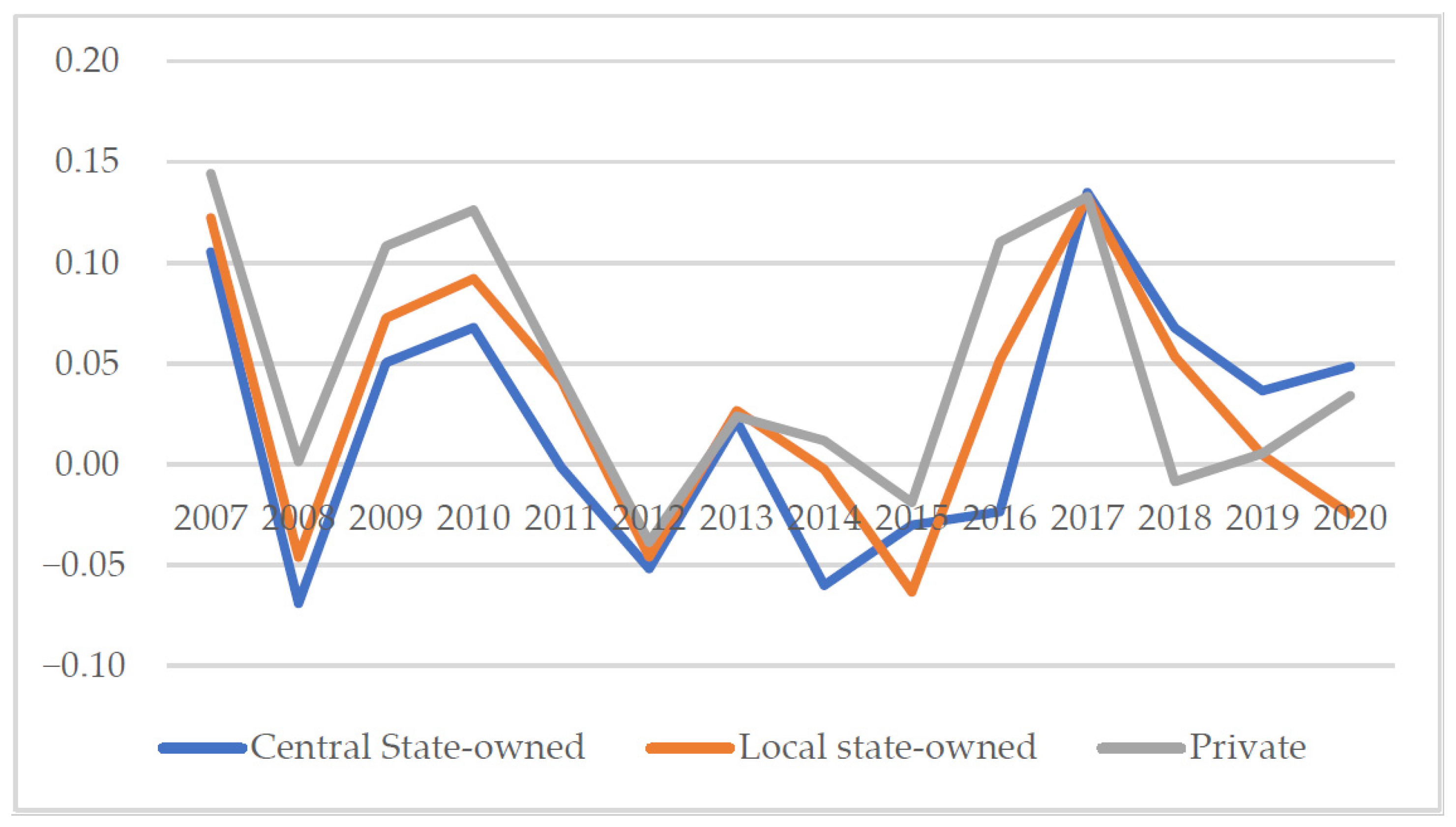
With the application of Stata 16.0, an SFA model based on the transcendental logarithmic production function was used to measure the enterprises’ TE; the average TE values for each year (from 2007 to 2020) are shown in Figure 1. Private enterprises have the overall highest mean value of TE, followed by the central and local SOEs. The overall trends of change in TE for all three enterprises during the thirteen-year period are roughly the same. In 2008, a significant plunge was followed by a climb over the following two years. TE declined significantly again in 2011 and 2012, fluctuated slightly during 2013–2015, increased in 2016–2018, then decreased. Notably, during 2017–2018, the TE of both the private enterprises and local SOEs decreased, whereas that of the central SOEs still maintained growth momentum, despite a low rate.
The following sections present comparative analyses of the preliminary TE measurements by industry and region. In terms of industry, the enterprises have been classified into labor-, capital-, and technology-intensive, according to the different percentages of their input factors. SOEs have different monopoly powers among these three industries, so we can analyze if the effects of their monopoly power on TE have really been negative. In terms of region, all the provinces, districts, and municipalities directly under the central government in mainland China have been divided into seven regions, so the comparison has analyzed if geographical factors affected TE and if the SOEs with really low TE were limited to particular regions or were distributed over the whole mainland.

5.1.1. Comparison of TE by Industry

All the listed enterprises were classified according to the three intensive industries, and their average TE values from 2007 to 2020 are shown in Table 4.
In terms of overall industry averages, capital-intensive industries have the highest TE, followed by labor- and technology-intensive. However, the TE of the private enterprises in the technology-intensive industries is higher than in the capital-intensive, because of the low TE of the central and local SOEs in the technology-intensive industries, especially that of the latter, which is only 0.49822 and pulls down the TE of the technology-intensive industries as a whole. In the labor-intensive industries, the TE of central SOEs, local SOEs and private enterprises are very close to the industry average (the gap between them and the industry average is less than 0.01). Therefore, the single factor ANOVA method is used to compare the TE differences of different ownership, because the concomitant probability of F statistic is 0.4254 > 0.1 (Table A3.). These industries have been reformed to a certain extent, to separate the government and enterprises, as the latter is the foundation of national economic life. However, 39 central SOEs and 118 local SOEs account for 78.89% of the overall number of enterprises, of which only 42 are private. This finding indicates that the monopoly power of SOEs still exists in the labor-intensive industries and puts up high barriers to entry for private enterprises. However, monopoly reduces the market competition faced by SOEs, while private enterprises can improve their competitiveness through layoffs. Therefore, the technical efficiency of state-owned enterprises and private enterprises in labor-intensive industries is almost the same.
For the capital-intensive industries, both the local SOEs and private enterprises have relatively high TE, whereas the central SOEs are relatively less technically efficient. The scale and crowding effects are two sides of the same coin, and agglomeration also leads to a transformation from the former to the latter [73]. In general, SOEs have more capital and scale resources, so they have certain advantages in terms of time and space, as well as efficiency. Therefore, when environmental interference factors are excluded, SOEs should be more efficient, as is reflected in the higher TE of the local SOEs. However, when the scale effect reaches a certain level, this can lead to an intra-industry crowding effect, with consequences such as large but single volumes of business, non-profit orientations of enterprise resources, or too many branch offices in an enterprise, all of which lead to a less than optimal allocation of production factors. The benefits of scale originally enjoyed by the central SOEs have become weaker than those of the local SOEs and private enterprises, which have been more flexible in resource allocation.
In the technology-intensive industries, the TE of the private enterprises is the highest, followed by those of the local and central SOEs, which still have certain advantages over the local SOEs. This is mainly because of the formers’ high-tech traits, strong innovation, high degree of industrial concentration, strong market competitiveness, the rapid elimination of private enterprises, and the higher requirements for product market competitiveness. When private enterprises cannot provide competitive products or services for a sustained period of time, they tend to be eliminated from the market, leaving behind those with relatively high TE and high output efficiency. Among the SOEs, the central ones undertake most of the scientific research tasks that are extremely important to the development of national science and technology. Additionally, they are supported by a high density of high-tech talents and strong government subsidies. For example, in 2020, the central SOEs in scientific research and technology services received subsidies totaling CNY 27,149,396,967.25, while local SOEs received CNY 25,932,459,902.26.

5.1.2. Comparison of TE by Region

China’s mainland is generally divided into seven geographical regions: northeastern (Heilongjiang, Jilin, and Liaoning Provinces), eastern (Shanghai City; Jiangsu, Zhejiang, Anhui, Fujian, Jiangxi, and Shandong Provinces), northern (Beijing and Tianjin Cities; Shanxi and Hebei Provinces; Inner Mongolia Autonomous Region), central (Henan, Hubei, and Hunan Provinces), southern (Guangdong and Hainan Provinces; Guangxi Zhuang Autonomous Region), southwestern (Sichuan, Guizhou, and Yunnan Provinces; Chongqing City; Tibet Autonomous Region), and northwestern (Shaanxi, Gansu, and Qinghai Provinces; Ningxia Hui and Xinjiang Uygur Autonomous Regions). Table 5 lists by descending order of average TE each type of enterprise in each region over a ten-year period.
The three regions with the highest mean TE are the northern, southern, and eastern. Beijing has made great contributions to the TE of northern China, with a mean value of 0.6739, which ranks second among all the provinces. The TE of southern China ranks second among all the regions. Here, Guangdong Province has made important contributions, with an average TE of 0.6150, which ranks fifth among all provinces. The average TE of eastern China is slightly lower than that of southern China. The main driving engine is Shanghai, with an average TE of 0.6955, which ranks first among all the provinces. However, the average TE of Anhui Province in eastern China is low, at only 0.5119, which lowers the overall level of the region’s TE, such that it ranks third among all the regions. Although the average TE of SOEs in eastern China is far lower than that in southern China, eastern China has the largest number of private listed enterprises among all the regions. During 2007 to 2020, 1185 observations accounted for 54.11% of the total number of private listed enterprises. With this huge base, the average TE of the private enterprises in eastern China remained at 0.6115, which has generally raised the TE level of all types of listed companies in the region. The average TE of the local SOEs in the top three regions is much higher than those in the remaining regions, but the differences in the TE of the private enterprises among the seven regions are not very large. In particular, the TE of central China’s central SOEs ranks fourth among the regions. However, the low level of the TE, at only 0.4526 of the local SOEs, leaves this region ranking last. Therefore, we can conclude that the level of the TE of the local SOEs largely determines the level of the whole region.
In recent years, the average value of the TE of the central SOEs in northeastern China has ranked fourth, mainly because the mean value of the TE of the central SOEs in Heilongjiang Province has only been 0.3451. Only the mean value of the TE of the central SOEs in the Ningxia Hui Autonomous Region is lower. The central SOEs in Heilongjiang Province involve only four industries, namely power, heat, gas, and water supply (the TE of one listed enterprise is 0.2959), agriculture, forestry, animal husbandry, and fishery (the TE of one listed enterprise is 0.3801), and manufacturing (the TE of two listed enterprises is 0.3840; the TE of one listed enterprise in the railway, ship, aerospace, and other transportation equipment manufacturing industry is 0.4636; and the TE of one listed enterprise in the chemical raw materials and chemical products manufacturing industry is 0.1923). The average TE of the central SOEs in the chemical raw materials and products manufacturing industry is only 0.1923, while the highest is 0.4636 in the railway, ship, aerospace, and other transportation equipment manufacturing industries. The average TE of the other two industries is within the range of 0.29–0.39.
The average TE of the central SOEs in these four industries in Heilongjiang Province is at a very low level. The province is located in the cradle of the old industrial base in northeastern China, the manufacturing industry of which used to be representative of the region’s economic competitiveness. However, in the past decade, the traditional manufacturing industry has faced the constraints and challenges of overcapacity, excessive debt burden, a weakening comparative advantage, and a declining position in the national industrial division of labor. However, the emerging manufacturing industry is small in scale and insufficient in capacity. The manufacturing industry has a structural imbalance, which hinders regional economic development. As a result, the TE of the central SOEs in the manufacturing industry of Heilongjiang Province is very low. In contrast, the TE is relatively high, mainly in Jilin Province, because the FAW Group’s subsidiary in this province is engaged in automobile manufacturing, which is one of the industries with the highest degree of automation. The average TE has reached 0.8530, which has raised the average level of the central SOEs in the manufacturing industry of Jilin Province.
Northwestern China is a vast area characterized by drought and water shortages, widespread deserts, a great deal of wind and sand, a fragile ecology, a sparse population, rich mineral resources, and underdevelopment. Therefore, this region has disadvantages in the level of the TE of all types of enterprises.

5.2. Decomposition and Comparison of TFP

A large difference exists between the total number of employees in the databases of some enterprises and the data of industrial added value after reduction in successive years. It is reasonable to suspect that abnormal values are present in the original data, which would make the calculated SC and AE values too large or too small, thereby affecting the stability of the results. Therefore, we removed 36 abnormal values with SC and AE greater than 5 or less than −5, which would account for 0.48% of the total number of 7500 records, to ensure the stability of the results, which are shown in Table 6.
Table 6 shows the TFP growth rate of all types of enterprises, from 2007 to 2020, as well as four decomposition parts, in which TEC represents the growth rate of TE. Since 2006 was used as the base year for calculating TE, SC, and AE, the information from that year was not considered.
Horizontal and vertical line graphs of the TFP growth rates from 2007 are shown in Figure 2. In the horizontal graph, the change trend of the TFP growth rate for private enterprises is the smoothest, and the mean value is the highest. In general, the TFP growth rates in 2020 are all lower than in 2007. In most years, all the enterprises were able to maintain their rates, which declined only in 2008, 2012, and 2014. The main reason is the negative TE change rates, which reduced the TFP growth rates. In 2008, the financial crisis reduced the TFP growth rates of all enterprises, but subsequent macroeconomic control by the state increased them in 2009, with the largest increase for private enterprises. The TFP growth rates of the central SOEs, local SOEs, and private enterprises reached their highest in 2017, at 0.1349, 0.1325, and 0.1327, respectively.
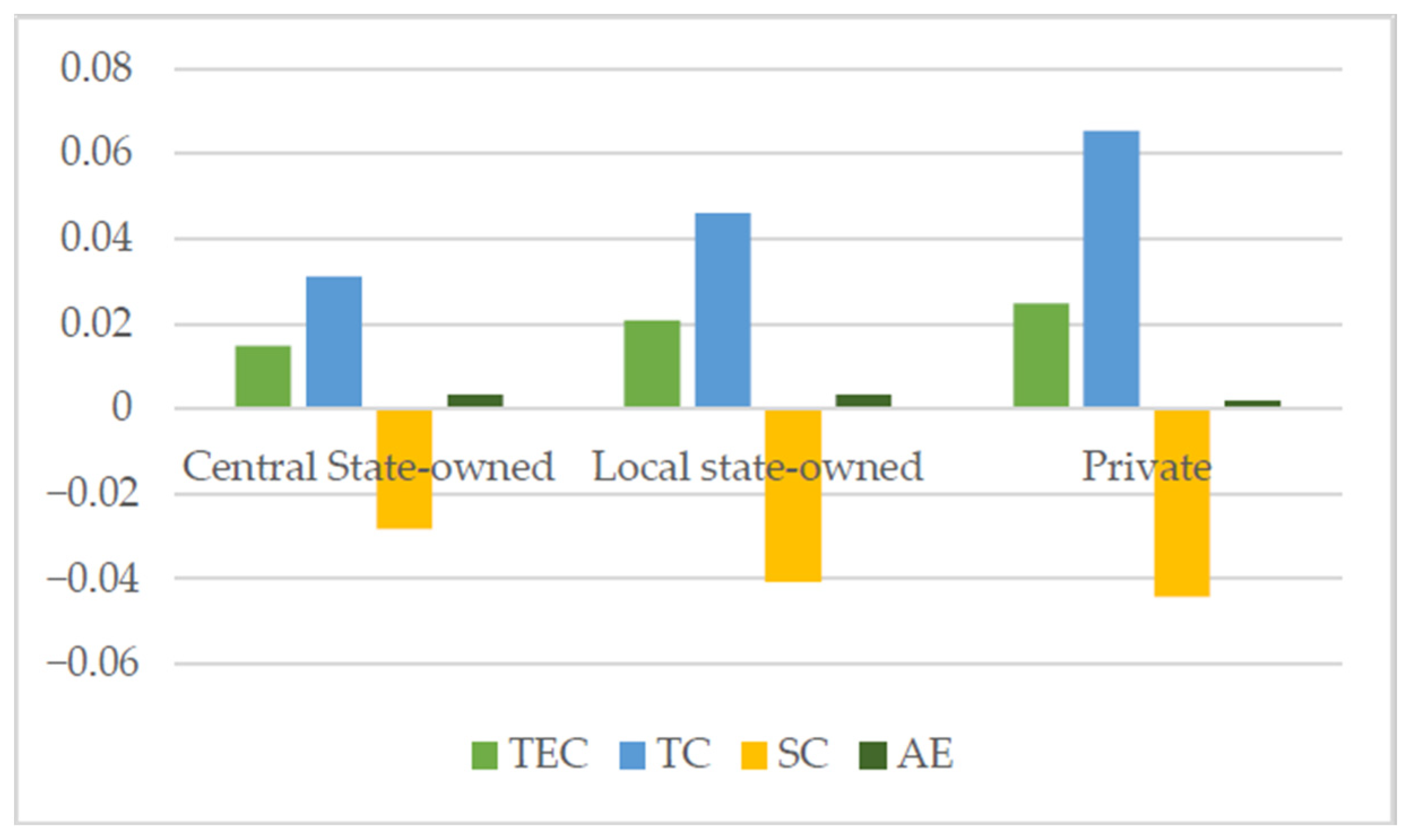
Figure 3 shows the mean values of the four decomposition parts of each type of enterprise. In terms of overall TE, all types experienced an increasing trend. In the horizontal graph, private enterprises had the highest mean rate of TE growth, followed by local and central SOEs. This situation may have been due to a series of policies, such as ‘invigorate the large enterprises while relaxing control over the small ones’ and ‘strategic adjustment’. Larger SOEs had been given more high-quality resources and were more dependent on government subsidies. In fact, these policies and the cheap credit provided to the SOEs resulted in changes in TE lower than those of the sampled private enterprises.
The changes in technological progress are positive in ascending order by the central SOEs, local SOEs, and private enterprises. This can be explained by the central SOEs being strongly directed by the central government, so they face little competition, and consequently, the motivation for technological progress is low. The local SOEs and private enterprises are motivated, due to the large enterprise base and fierce competition.
In contrast with changes in TE and technological progress, scale efficiency depresses the growth rate of TFP. Changes in scale efficiency were all negative in ascending order by private enterprises, local SOEs, and central SOEs (−0.0283). After the downsizing of the central SOEs by the State-Owned Assets Supervision and Administration Commission (SASAC), they are no longer large central enterprises that have significant control over important industries of the national economy and over people’s livelihoods; nor do they have strong driving forces in new energy, new materials, aerospace, intelligent manufacturing, and other industries. The central enterprises generally adopt overall listing and operate the whole group as a listed company. The resources between the group and its subsidiaries, as well as among departments, can be better integrated as upstream and downstream are combined. As a result, average costs and operational risks are reduced, in order to realize external economies of scale. As a whole, improvements in scale efficiency have great potential to boost TFP.
The factor allocations have improved to a relatively small extent. The factor allocation efficiency of both SOEs has improved faster than that of the private enterprises, indicating that the significant marketization process of China’s economy has also gradually improved the marketization degree of the private enterprises, so the market can reasonably and effectively allocate resources. Nonetheless, the AE of the SOEs is lower, which may be due to the fact that the SOEs have long been an important means by which China’s central and local governments have participated in the market. Consequently, the SOEs undertake social functions, such as facilitating stable employment. Their market-oriented reforms are challenging [53]. The SOEs and the private enterprises differ greatly in terms of obtaining resources and receiving factor prices. This mechanism has hindered the free flow of production factors to a certain extent and has resulted in the allocation efficiency of the SOEs not reaching the growth rate of the private enterprises.

5.2.1. Comparison of TFP Decompositions

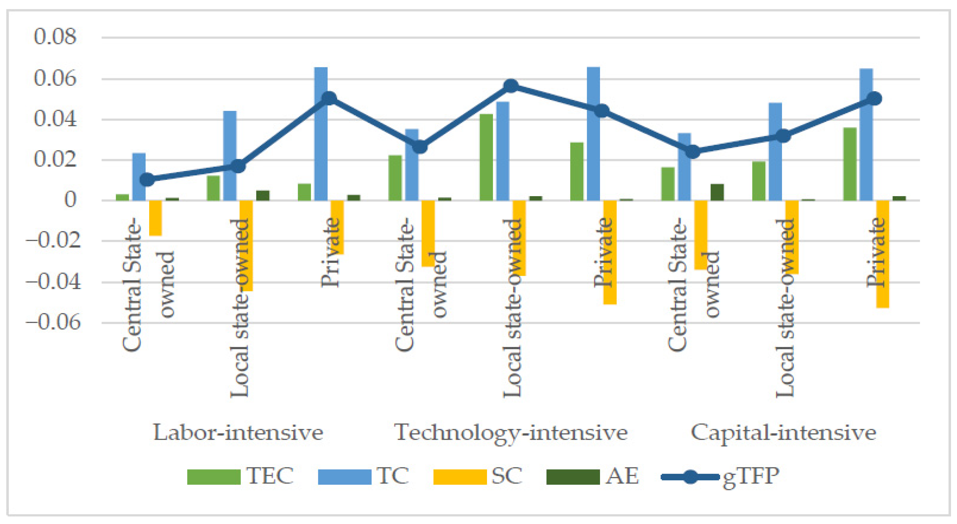
Figure 4 shows the average values of the four components.
The SC of all industries is negative, indicating that the SC has hindered the growth of TFP. For the central SOEs, the TFP growth rate is relatively low in the labor-intensive industries (0.0104) but relatively high in the technology-intensive (0.0265) and capital-intensive industries (0.0240). The decomposition indices of the TFP growth rates show that the main factors hindering the rates of the central SOEs in the labor-intensive industries are the TEC (0.0031) and TC (0.0233), which are far lower than in the other industries. Therefore, the central SOEs should attach importance to the improvement of TE and TC in the labor-intensive industries. They should also effectively increase the TFP growth rates by increasing investments in technological innovation. Similarly, the TFP growth rates of the local SOEs are the lowest in the labor-intensive industries (0.0169), highest in the technology-intensive industries (0.0563), and medium in the capital-intensive (0.0319) industries. A comparison of the decomposition indices of the TFP growth rates by industry shows that low EC and SC are the main factors that hinder the TFP growth rates of the labor-intensive industries. In the capital-intensive industries, the TFP growth rates are lower than that of the technology-intensive industries, mainly because of low TEC. For private enterprises, the TFP growth rates in all industries are relatively similar and high at about 0.05. The TEC of the labor-intensive industries is significantly lower than those of the other two. In the technology- and capital-intensive industries, SC decreases significantly, by −0.0510 and −0.0527, respectively, which seriously affects the improvement of the TFP growth rates.
The labor-intensive industries have the lowest TEC and smallest decrease in SC, suggesting that the TFP growth rates currently rely mainly on the maintenance of the scale effect, rather than the increase in TE. The scale effect of the local SOEs is the lowest, but their resource allocation efficiency is the highest. The technology-intensive industries have the highest increase in TEC (0.0425 for local SOEs), and the highest rate of TC, (0.06566 for private enterprises). These findings suggest that the high degree of openness and intensity of competition has provided incentives for innovation and TEC. The scale effect of private enterprises decreases the most, followed by local SOEs. In the capital-intensive industries, private enterprises have the largest decrease SC at −0.0527, as well as the highest TEC and TC. Since the marketization in China has been on track, the domestic economy has undergone a transformation from undersupply to oversupply. Market competition has become increasingly fierce since the economic reforms and liberalization, so enterprises must invest more in technological innovation and improve their efficiency. Private enterprises have recognized the importance of technology and have taken the path of development largely driven by technology rather than scale.

5.2.2. Decomposition and Comparison

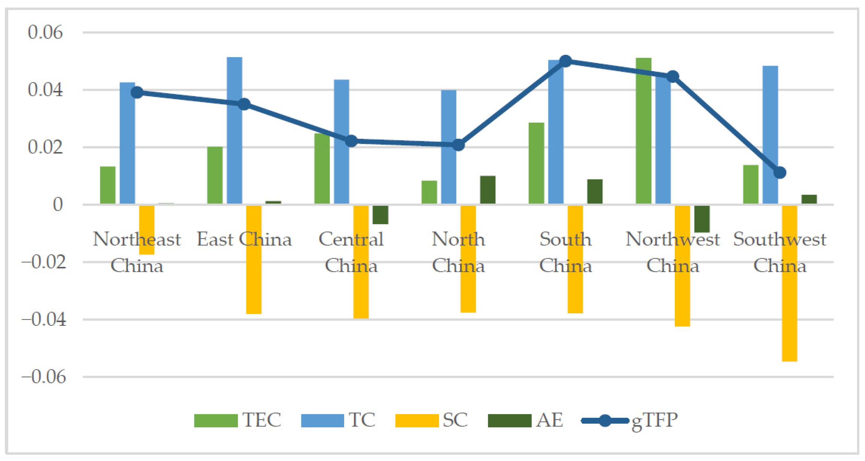
Figure 5 shows the decomposition results of the TFP growth rates in each region.
In general, the TFP growth rates in various regions have been supported by TEC and TC, which have especially been the most important contributing factors. The TEC of each region is positive, with the highest being 0.0512 in northwestern China, while those in eastern, central, and southern China are higher than 0.02. The TC of each region is higher than 0.04, with the highest being 0.0514 in eastern China. The SC is negative in all regions, indicating that improvement is required. The AE is negative in central and northwestern China, indicating that the matching ratios of the factors in these regions are unreasonable. In northern and southern China, the AE is higher, at 0.0100 and 0.0089, respectively, which indicates effective contributions to their TFP growth rates.
A comparison of the average regional TE shows that the TFP growth rate in southern China (0.0501) is the highest. Its average TE is also high, ranking second. The average growth rate of TFP in northwestern China is relatively high, also ranking second, but the average TE is relatively low, ranking third from the bottom. In contrast, the average TFP growth rate in northern China is relatively low, ranking sixth, whereas the average TE is high, ranking first.
The changes in TE and TC in northeastern and southwestern China are similar, but their TFP growth rates rank quite differently, mainly because of the large difference in their SC. The SC in southwestern China decreased by −0.0546, which has seriously affected the increase in that region’s TFP growth rate. However, the SC in northeastern China has the smallest decrease of −0.0173, which ranks the region’s TFP growth rate relatively high.

6. Conclusions

This study uses stochastic frontier analysis (SFA), a transcendental logarithmic production function, and the industrial added value and labor input data (from 2006 to 2020) of listed central state-owned enterprises (SOEs), local SOEs, and private enterprises. The data are used to calculate the enterprises’ technical efficiency (TE). In addition, we divided the growth rate of total factor productivity (TFP) into four components: TE change (TEC), technical change (TC), scale change (SC), and allocation efficiency change (AE). The conclusions are as follows:
First, the private enterprises have the highest TE, followed by the central and local SOEs. The TFP growth rate of the private enterprises is the most stable but has declined overall. The TEC and TC of the private enterprises are also the highest, followed by the local and central SOEs. However, the SC and AE of the central SOEs are better than those of the private enterprises.
Second, a cross-industry comparison of the labor-, capital-, and technology-intensive industries shows that the TFP growth rates of the central SOEs were relatively low in the labor-intensive industries, mainly because of the low TEC and TC. Therefore, increasing investment in technological innovation would be urgently required. The main reasons for the low TFP growth rates in the labor-intensive enterprises are the low TEC and SC of the local SOEs. The TFP growth rates of private enterprises in all three industries are higher than the average levels. The TFP growth rates of the labor-intensive industries mainly depend on the maintenance of SC, rather than the improvement of TE. The technology-intensive industries actively engage in TC and have high TE. In the capital-intensive industries, the decreases in the SC of the central and local SOEs are smaller, but their TEC and TC are lower than those of private enterprises.
Third, a cross-regional comparison shows that the local SOEs in a region largely determined that region’s TE level during the study period. Northern China has the highest TE, and southern China has the highest TFP growth rate. Eastern China has the highest number of private enterprises, which the region relies on to raise its level of TC.
The overall efficiency of China’s SOEs is relatively low. The results of this study provide China’s interpretation of the international experience, based on the theory of property rights and monopoly. The main point of monopoly theory is that monopoly creates economic profits, rather than competition. Therefore, enterprises that enjoy a monopoly lack the power to reduce costs and innovate technology, which leads to inefficiency. This situation is common in both Western countries and China. Peterson and Lewis believed that the existence of monopolistic enterprises was not threatened, because these enterprises could obtain monopoly-based profits, even if their costs increased [74]. The view of property right theory is that the ownership of SOEs belongs to all members of society, but the theory is not specific regarding who exercises the ownership rights on behalf of all members of society. This leads to unclear property rights, unclear responsibilities, and the absence of owners, which, in turn, causes the operators of SOEs to lack effective incentives and constraints, ultimately affecting the overall efficiency of SOEs. Dilorenzo and Robinson [75], and Atkinson and Halvorsen [76] concluded that the low efficiency of SOEs was mainly due to the capital subsidies received by those enterprises.
Our results convey some messages for policymakers. To a certain degree, the central SOEs are more efficient than the local SOEs, which should learn from the central SOEs in terms of the direction of deepening reforms. Listed companies still have much room to achieve sustainable growth through the improvement of TFP. From the perspective of property rights theory, through the supervision and incentive mechanism, the reform of SOEs can ensure that the residual claim and residual control rights of managers during their tenure partially correspond to each other. This would reduce the SOEs’ loss of efficiency. Moreover, SOEs should consider making use of their scale advantages to put more effort into technological development, and technological innovation should be promoted. From the perspective of monopoly theory, this paper recommends that the industries in which the SOEs have high degrees of monopoly should improve the degree of openness and allow the market to develop high-intensity competition to a certain extent. The acceleration of marketization, allowance of the rational and free flow of factors and resources between SOEs and non-SOEs, and improvement of the factor allocation efficiency of the SOEs are necessary. Local SOEs and private enterprises should also learn from the central SOEs, strengthen the integration of the various links and linkages between upstream and downstream, and improve the external scale effect.
This study has some limitations. We did not further compare the efficiency of SOEs in multiple economies. Moreover, we used the transcendental logarithmic production function, but did not consider the case of multiple outputs. These will be the direction of future research in this field.

Author Contributions

Conceptualization, C.L. and D.L.; Methodology, C.L. and J.L.; Software, J.L.; Investigation, C.L., D.L. and K.H.; Data Curation, J.L., M.J. and K.H.; Writing—original draft preparation, D.L. and M.J.; Writing—review and editing, C.L.; Visualization, M.J.; Supervision, C.L.; Funding acquisition, C.L. All authors have read and agreed to the published version of the manuscript.

Funding

This research was funded by the National Social Science Foundation of China: Research on Structural Optimization of Innovation Elements in the Old Industrial Base under Supply-side Structural Reform, grant number 21BGL304.

Data Availability Statement

Publicly available datasets were analyzed in this study. This data can be found here: [https://www.wind.com.cn/]. [https://www.gtarsc.com]. [http://www.stats.gov.cn/tjsj/ndsj/], accessed on 17 January 2023.

Conflicts of Interest

The authors declare no conflict of interest.

Appendix A

Table A1. Descriptive stati stics.
tlnylnklnlt2lnk2lnl2lnklnltlnktlnl
Mean8.52910.85011.5708.22189.000136.80069.21096.610100.10071.310
Median9.00010.77011.4478.24881.000131.03468.03294.00596.96669.646
Minimum2.0004.4604.6962.7084.00022.0507.33421.28011.7205.416
Maximum15.00017.34017.96013.020225.000322.700169.500233.500265.600192.900
Std. dev.4.0331.4311.6961.27470.15040.15020.95026.79052.03037.240
Skewness−0.0080.3930.201−0.1170.5200.8230.5550.7310.2490.227
Kurtosis1.7873.9233.9953.9872.0004.6004.2544.7962.1012.090
Jarque–Bera test416.8 ***416.4 ***326.3 ***291.6 ***589.7 ***1492 ***794 ***1518 ***298.9 ***292.6 ***
Observations6794679467946794679467946794679467946794
Note: *** indicate significance at the 1% and 5% levels, respectively.
Table A2. Correlation matrix.
Variableslnytlnklnlt2lnk2lnl2lnklnltlnktlnl
lny1
t0.282 ***1
lnk0.711 ***0.202 ***1
lnl0.631 ***0.232 ***0.678 ***1
t20.273 ***0.979 ***0.195 ***0.217 ***1
lnk20.732 ***0.201 ***0.992 ***0.671 ***0.194 ***1
lnl20.657 ***0.225 ***0.691 ***0.991 ***0.212 ***0.692 ***1
lnklnl0.747 ***0.234 ***0.903 ***0.916 ***0.222 ***0.907 ***0.929 ***1
tlnk0.452 ***0.951 ***0.466 ***0.398 ***0.935 ***0.465 ***0.397 ***0.468 ***1
tlnl0.437 ***0.952 ***0.379 ***0.486 ***0.935 ***0.378 ***0.482 ***0.472 ***0.970 ***1
Note: *** indicate significance at the 1% and 5% levels.
Table A3. Single factor ANOVA table for labor-intensive industries.
Source of VariationSSdfMSFp-ValueF Crit
Between groups0.106520.05320.85500.42542.9987
Within groups187.567730120.0623
Total187.67423014
Table A4. Variables definition.
VariableDescription
tTime trends.
lnyitLogarithms of the output of the listed company i (i = 1, 2, …, N; t = 1, 2, …, 10) in year t.
lnkitLogarithms of the capital of the listed company i (i = 1, 2,…,N; t = 1, 2, …, 10) in year t.
lnlitLogarithms of the labor of the listed company i (i = 1, 2, …, N; t = 1, 2, …, 10) in year t.
vitRandom error, reflecting the non-efficiency of the system.
uitTechnical loss error, reflecting technical inefficiency.
Number of dmuNumber of enterprises in each model. Each enterprise has 15 years of data, from 2006 to 2020, which is a balanced panel.
γ γ = σ u 2 σ u 2 + σ v 2 , γ is the proportion of technical invalid rate in random disturbance term; when γ approaches 1, this shows that the error of SFA estimation is mainly due to the loss of technical efficiency, and SFA fits the production function model well.

References

  1. Wang, Y.; Chen, C.; Gao, S. Estimation and Analysis of China’s Urban Total Factor Productivity: 2000–2013. Econ. Issues 2016, 1–8. [Google Scholar] [CrossRef]
  2. Douglass, C.N. Structure and Change in Economic History; Shanghai People’s Publishing House: Shanghai, China, 1994; p. 186. [Google Scholar]
  3. Sun, X.; Wang, Y. Firm nature, R & D efficiency and total factor productivity: An Empirical Test Based on micro data of Chinese industrial enterprises. J. Dalian Univ. Technol. (Soc. Sci. Ed.) 2014, 35, 35–41. [Google Scholar]
  4. Hsieh, C.T.; Klenow, J.P. Misallocation and Manufactuting TFP in China and India. Q. J. Econ. 2009, 124, 1403–1448. [Google Scholar] [CrossRef] [Green Version]
  5. Nie, H.; Jia, R. Productivity and Resource Misplacement of Chinese Manufacturing Enterprises. World Econ. 2011, 34, 27–42. [Google Scholar]
  6. The State Council of the People’s Republic of China. The 14th Five-Year Plan for the National Economic and Social Development of the People’s Republic of China and Outline of Long-Term Goals for 2035. Available online: http://www.gov.cn/xinwen/2021-03/13/content_5592681.htm (accessed on 16 June 2021).
  7. The State Council of the People’s Republic of China. Xi Jinping: Secure a Decisive Victory in Building a Moderately Prosperous Society in all Respects, Strive for the Great Success of Socialism with Chinese Characteristics for a New Era-Report at the 19th National Congress of the Communist Party of China. Available online: http://www.gov.cn/zhuanti/2017-10/27/content_5234876.htm (accessed on 16 June 2021).
  8. Djankov, S.; Murrell, P. Enterprise restructuring in transition: A quantitative survey. J. Econ. Lit. 2002, 40, 739–792. [Google Scholar] [CrossRef]
  9. Estrin, S.; Hanousek, J.; Kocenda, E.; Svejnar, J. The Effects of Privatization and Ownership in Transition Economies. J. Econ. Lit. 2009, 47, 699–728. [Google Scholar] [CrossRef] [Green Version]
  10. Brown, J.D.; Earle, J.S.; Telegdy, Á. The Productivity Effects of Privatization: Longitudinal Estimates from Hungary, Romania, Russia, and Ukraine. J. Political Econ. 2006, 114, 61–99. [Google Scholar] [CrossRef] [Green Version]
  11. Bogart, D.; Chaudhary, L. Off the rails: Is state ownership bad for productivity? J. Comp. Econ. 2015, 43, 997–1013. [Google Scholar] [CrossRef] [Green Version]
  12. Curtis, C. Economic Reforms and the Evolution of China’s total factor productivity. Rev. Econ. Dyn. 2016, 21, 225–245. [Google Scholar] [CrossRef]
  13. Coelli, T.; Rao, D.S.P.; Battese, G.E. An Introduction to Efficiency and Productivity Analysis; Kluwer Academic Publishers: Boston, MA, USA, 1998. [Google Scholar] [CrossRef]
  14. Shen, C.; Zhao, S. Research on the impact of market competition and non-interest business on the efficiency of commercial banks. J. Quant. Technol. Econ. 2017, 34, 145–161. [Google Scholar] [CrossRef]
  15. Tao, H.; Tian, J.; Hao, S. Time series analysis of operational efficiency of state-owned enterprises based on DEA method-Comparison with private enterprises. Theor. J. 2012, 48–52. [Google Scholar] [CrossRef]
  16. Wu, H.; Li, D. Total Factor Productivity Growth Comparison of Domestic and Foreign Enterprises in China’s Manufacturing Industry. Syst. Eng. 2012, 30, 92–97. [Google Scholar]
  17. Guo, C.; Chen, C. Research on the difference of total factor productivity in manufacturing industry-based on the distribution and change of manufacturing scale. Price Theory Pract. 2018, 143–146. [Google Scholar] [CrossRef]
  18. Xu, S.; Du, D.; Gui, Q.; Qin, X. Is the Technological Progress of Foreign Economy Better than that of Private Economy? Empirical Research on Total Factor Productivity in Shanghai. Res. Dev. Manag. 2019, 31, 115–125. [Google Scholar] [CrossRef]
  19. Aigner, D.; Lovell, C.A.K.; Schmidt, P. Formulation and Estimation of Stochastic Frontier Production Function Models. J. Econom. 1977, 6, 21–37. [Google Scholar] [CrossRef]
  20. Meeusen, W.; van den Broeck, J. Technical Efficiency and Dimension of the Firm: Some Results on the Use of Frontier Production Functions. Empir. Econ. 1977, 2, 109–122. [Google Scholar] [CrossRef]
  21. Kuang, Y. Technical Efficiency, Technical Progress, Factor Accumulation and China’s Agricultural Economic Growth—Empirical Analysis Based on SFA. Res. Quant. Econ. Tech. Econ. 2012, 29, 3–18. [Google Scholar] [CrossRef]
  22. Li, G.; Feng, Z.; Fan, L. Decomposition of technical efficiency of household operation and total factor productivity growth (1999–2003)—Based on stochastic frontier production function and micro evidence from farmers in Hubei Province. Res. Quant. Econ. Tech. Econ. 2007, 24, 25–34. [Google Scholar]
  23. Oh, S.-C.; Shin, J. The Assessment of Car Making Plants with an Integrated Stochastic Frontier Analysis Model. Mathematics 2021, 9, 1296. [Google Scholar] [CrossRef]
  24. Li, X.; Qin, J.; Sun, L. The dynamic changes of operating environment, governance structure and total factor productivity of commercial banks. China Ind. Econ. 2014, 57–68. [Google Scholar] [CrossRef]
  25. Zheng, S.; Yin, X. Diversification analysis of China’s commercial banks based on the perspective of X efficiency. Quant. Econ. Tech. Econ. Res. 2013, 30, 81–97. [Google Scholar] [CrossRef]
  26. Jiang, P.; Wang, Y. Research on the input-output efficiency of China’s cultural industry in full caliber-Analysis based on three-stage DEA model and super-efficiency DEA model. Quant. Econ. Tech. Econ. Res. 2011, 28, 69–81. [Google Scholar] [CrossRef]
  27. Wang, D.; Li, J. China’s tax collection efficiency and its influencing factors-Empirical research based on stochastic frontier analysis (SFA) technology. Quant. Econ. Tech. Econ. Res. 2009, 26, 152–161. [Google Scholar]
  28. Zhu, B.; Song, Z. Research on performance evaluation of open-end funds in China based on SFA efficiency value. Quant. Econ. Tech. Econ. Res. 2009, 26, 105–116. [Google Scholar]
  29. Gan, X. Empirical Analysis of the Efficiency Structure of China’s Insurance Industry. Quant. Econ. Tech. Econ. Res. 2008, 92–105. [Google Scholar]
  30. Yang, Q.; Su, Q.; Yin, L. China’s service industry productivity and its influencing factors-Empirical research based on stochastic frontier production function. Quant. Econ. Tech. Econ. Res. 2009, 26, 46–57. [Google Scholar]
  31. Gu, N. The impact and channels of producer services on industrial profitability-an empirical study based on urban panel data and SFA model. China Ind. Econ. 2010, 48–58. [Google Scholar] [CrossRef]
  32. Xing, H.; Gao, J.; Tan, H. International spatial spillover and total factor productivity of service industry-Measurement based on spatial stochastic frontier analysis method. Quant. Econ. Tech. Econ. Res. 2021, 38, 75–95. [Google Scholar] [CrossRef]
  33. Zhu, Y.; Xu, K. Empirical Study on R&D Efficiency of High-tech Industry in China. China Ind. Econ. 2006, 38–45. [Google Scholar] [CrossRef]
  34. Bai, J.; Bian, Y. Factor market distortions and efficiency loss of innovative production in China. China Ind. Econ. 2016, 39–55. [Google Scholar] [CrossRef]
  35. Sun, W.; Shen, K. Difference between Human Capital Accumulation and Technological Innovation Efficiency of Chinese Manufacturing Industry. China Ind. Econ. 2009, 81–91. [Google Scholar] [CrossRef]
  36. Han, Z.; Cheng, X. Measurement and Analysis of Provincial R&D Input and Innovation Efficiency in China. Quant. Econ. Tech. Econ. Res. 2020, 37, 98–117. [Google Scholar] [CrossRef]
  37. Shi, X.; Zhao, S.; Wu, F. China’s regional innovation efficiency and its spatial differences. Quant. Econ. Tech. Econ. Res. 2009, 26, 45–55. [Google Scholar]
  38. Dai, Y. China’s urbanization efficiency and its influencing factors-Analysis based on stochastic frontier production function. Quant. Econ. Tech. Econ. Res. 2010, 27, 103–117. [Google Scholar] [CrossRef]
  39. Zhang, G.; Xia, D. Ownership structure, environmental regulation and the efficiency of China’s power generation industry—Analysis based on 30 provincial panel data from 2003 to 2009. China Ind. Econ. 2011, 130–140. [Google Scholar] [CrossRef]
  40. Yuan, Y.; Guo, L.; Sun, J. Structure, Technology, Management and Energy Efficiency-An Analysis Based on China’s Provincial Panel Data from 2000 to 2010. China Ind. Econ. 2012, 18–30. [Google Scholar] [CrossRef]
  41. Zhang, S.; Jiang, W. Energy Efficiency Measurement Method: Evolution, Controversy and the Future. Quant. Econ. Tech. Econ. Res. 2016, 33, 3–24. [Google Scholar] [CrossRef]
  42. Lin, B.; Du, K. The impact of factor market distortions on energy efficiency. Econ. Res. 2013, 48, 125–136. [Google Scholar]
  43. Sun, C.; Lin, B. China’s industrial energy factor allocation efficiency and energy saving potential research. Quant. Econ. Tech. Econ. Res. 2014, 31, 86–99. [Google Scholar] [CrossRef]
  44. Jiang, Y.; Zhu, G. Technical inefficiency of energy use and its convergence analysis. Quant. Econ. Tech. Econ. Res. 2007, 24, 108–119. [Google Scholar]
  45. Duan, W.; Liu, D.; Yu, Y. Technical path and comparative advantage of energy saving and emission reduction in heterogeneous industries-theoretical model and empirical test. China Ind. Econ. 2013, 69–81. [Google Scholar] [CrossRef]
  46. Li, D.; Hu, X. Research on Relative Efficiency and Total Factor Productivity Growth of Chinese Manufacturing Enterprises-An Empirical Analysis Based on Industry Data from 1999 to 2005. Quant. Econ. Tech. Econ. Res. 2008, 25, 31–41. [Google Scholar]
  47. Zheng, S.; Kjetil, S.; Fabrizio, Z. Growing Like China. Am. Econ. Rev. 2011, 101, 196–233. [Google Scholar]
  48. Hao, S.; Tao, H.; Tian, J. A comparative study on the governance efficiency of state-owned enterprises with different ownership structures: A case study of Shandong Province. China Ind. Econ. 2011, 130–139. [Google Scholar]
  49. Fan, J.; Yu, X.; Zhao, L. A study on the regional efficiency differences among state-owned, private and foreign-funded industrial enterprises in China. Quant. Econ. Tech. Econ. Res. 2015, 32, 21–38. [Google Scholar]
  50. Xu, B. Analysis of efficiency loss of state-owned enterprises. Tech. Econ. Manag. 2017, 56–60. [Google Scholar]
  51. Berkowitz, D.; Ma, H.; Nishioka, S. Recasting the iron rice bowl: The reform of China’s state-owned enterprises. Rev. Econ. Stat. 2017, 99, 735–747. [Google Scholar] [CrossRef]
  52. Zhang, T.; Liu, K.; Xiong, X. A comparative study on the production efficiency of Chinese state-owned enterprises and private enterprises. Quant. Econ. Tech. Econ. Res. 2018, 35, 78–94. [Google Scholar]
  53. Li, Y.; Yang, R. Dependence of local state-owned enterprises, improvement of resource allocation efficiency and supply side Reform. Econ. Res. 2018, 53, 80–94. [Google Scholar]
  54. Wang, W.; Liu, X. Why zombie enterprises can survive for a long time. China Ind. Econ. 2018, 61–79. [Google Scholar]
  55. Yin, Z.; Liu, L.; Wang, H. Study on the ownership balance and the efficiency of mixed ownership enterprises from the perspective of heterogeneous shareholders. PLoS ONE 2018, 13, e0194433. [Google Scholar] [CrossRef] [Green Version]
  56. Liu, Z.; Spiegel, M.M.; Zhang, J. Optimal capital account liberalization in China. J. Monet. Econ. 2021, 117, 1041–1061. [Google Scholar] [CrossRef]
  57. Zhao, Q. Are state-owned enterprises really inefficient—From the perspective of regional innovation efficiency spillover effect. Sci. Sci. Manag. Sci. Technol. 2017, 38, 107–116. [Google Scholar]
  58. Zhao, T.; Fang, H. Empirical Study on OFDI and China’s innovation efficiency. Quant. Econ. Tech. Econ. Res. 2019, 36, 58–76. [Google Scholar]
  59. Tan, T.; Wu, J.; Wang, M.K.; Shen, W. Research on the efficiency of commercial banks in countries along the “21st century Maritime Silk Road”. Quant. Econ. Tech. Econ. Res. 2020, 37, 60–77. [Google Scholar]
  60. Kong, D.; Tang, Q.; Xiang, J. Labor protection and labor investment efficiency of enterprises. J. Huazhong Univ. Sci. Technol. (Soc. Sci. Ed.) 2020, 34, 36–47. [Google Scholar]
  61. Levinsohn, J.; Petrin, A. Estimating Production Functions using Inputs to Control for Unobservables. Rev. Econ. Stud. 2003, 70, 317–341. [Google Scholar] [CrossRef]
  62. Olley, G.S.; Pakes, A. The Dynamics of Productivity in the Telecommunications Equipment lndustry. Econometrica 1996, 64, 1263–1297. [Google Scholar] [CrossRef]
  63. Fu, X.; Wu, L. Applicability of frontier analysis method in China’s economic growth accounting. World Econ. 2007, 30, 56–66. [Google Scholar]
  64. Battese, G.E.; Coelli, T.J. A model for technical inefficiency effects in a stochastic frontier production function for panel data. Empir. Econ. 1995, 20, 325–332. [Google Scholar] [CrossRef] [Green Version]
  65. Kumbhakar, S.C. Estimation and Decomposition of Productivity Change When Production is not Efficient: A Panel Data Approach. Econom. Rev. 2000, 19, 425–460. [Google Scholar] [CrossRef]
  66. Tu, Z.; Xiao, G. Industrial Productivity Revolution in China—Decomposition and Analysis of Total Factor Productivity Growth of Large and Medium-sized Industrial Enterprises in China by Stochastic Frontier Production Model. Econ. Res. 2005, 40, 4–15. [Google Scholar]
  67. National Bureau of Statistics. China Statistical Yearbook. Available online: http://www.stats.gov.cn/tjsj/ndsj/ (accessed on 5 September 2021).
  68. Lu, T.; Dang, Y. Corporate governance and technological innovation: Comparison by industry. Econ. Res. 2014, 49, 115–128. [Google Scholar]
  69. Industry classification guidelines for listed companies. Available online: http://www.csrc.gov.cn/csrc/c100103/c1452025/content.shtml (accessed on 16 September 2021).
  70. Batrancea, L.; Rathnaswamy, M.K.; Batrancea, I. A Panel Data Analysis on Determinants of Economic Growth in Seven Non-BCBS Countries. J. Knowl. Econ. 2022, 13, 1651–1665. [Google Scholar] [CrossRef]
  71. Batrancea, L.M. An Econometric Approach on Performance, Assets, and Liabilities in a Sample of Banks from Europe, Israel, United States of America, and Canada. Mathematics 2021, 9, 3178. [Google Scholar] [CrossRef]
  72. Batrancea, L. The Influence of Liquidity and Solvency on Performance within the Healthcare Industry: Evidence from Publicly Listed Companies. Mathematics 2021, 9, 2231. [Google Scholar] [CrossRef]
  73. Zhou, S.; Zhu, W. Can Industrial Clustering Bring Economic Efficiency: Scale Effect and Congestion Effect. Res. Ind. Econ. 2013, 12–22. [Google Scholar] [CrossRef]
  74. Craig Petersen, H.; Cries Lewis, W. Managerial Economies, 3rd ed.; MacMillan Publishing Company: New York, NY, USA, 1994. [Google Scholar]
  75. DiLorenzo, T.J.; Robinson, R. Managerial objectives subject to political market constraints: Electric utilities in the US. Q. Rev. Bus. Econ. 1982, 22, 113–125. [Google Scholar]
  76. Atkinson, S.E.; Halvorsen, R. The relative efficiency of public and private firms in a regulated environment: The case of US electric utilities. J. Public Econ. 1986, 29, 281–294. [Google Scholar] [CrossRef]
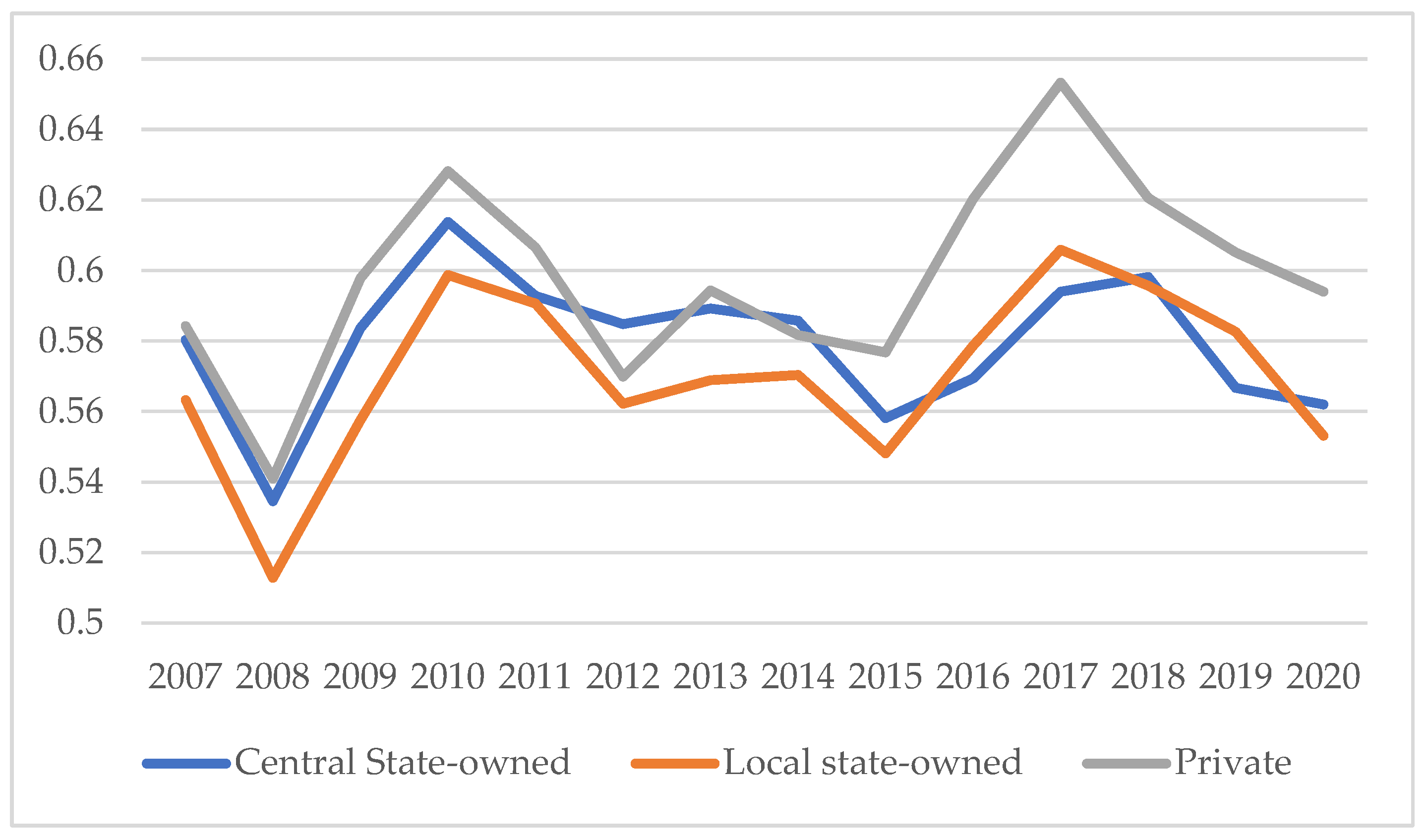
Figure 1. Trends of technical efficiency change of enterprises under all kinds of ownership in 2007–2020.
Mathematics 11 00657 g001
Figure 2. Change chart of TFP growth rates by ownership enterprises.
Mathematics 11 00657 g002
Figure 3. TFP decomposition by ownership enterprises.
Mathematics 11 00657 g003
Figure 4. Bar chart of SFA decomposition results with regard to ownership enterprises of different industries.
Mathematics 11 00657 g004
Figure 5. Decomposition diagram of TFP of listed companies by region.
Mathematics 11 00657 g005
Table 1. Descriptive statistics of relevant indicators of listed enterprises with three kinds of ownership.
Central State-OwnedLocal State-OwnedPrivate Enterprise
VariablelnYlnKlnLlnYlnKlnLlnYlnKlnL
Mean11.0511.98.42310.8711.628.08910.4111.068.057
Std. Dev.1.6542.0721.3931.3491.6111.3381.3091.3091.116
Min5.6744.6963.4666.2355.432.7084.465.0613.178
Max17.3417.9613.0215.6416.0112.2914.2914.7111.47
N192019201920339033903390219021902190
Table 2. Industry classifications by factor intensity.
Labor-IntensiveCapital-IntensiveTechnology-Intensive
A Agriculture, forestry, animal husbandry and fishery
B Mining industry
C13 Processing of food from agricultural products
C14 Manufacture of foods
C15 Wine, beverage and refined tea manufacturing
C17 Manufacture of textile
C18 Manufacture of textile wearing apparel and fashion
C19 Manufacture of leather, fur, feather and related products, manufacture of footwear
C20 Processing of timber, manufacture of wood, bamboo, rattan, palm and straw products
C21 Manufacture of furniture
D Production and supply of electric power, heat power, gas and water
E Construction industry
F Wholesale and retail trade
G Transportation, warehousing and postal services
R Culture, sports and entertainment industry
S Comprehensive
C22 Manufacture of paper and paper products
C23 Printing, reproduction of recording media
C24 Culture and education, art, sports and recreation goods manufacturing
C25 Processing of petroleum, coking, processing of nuclear fuel
C26 Manufacture of raw chemical materials and chemical products
C28 Manufacture of chemical fibers
C29 Manufacture of rubber and plastics
C30 Manufacture of non-metallic mineral products
C31 Smelting and pressing of ferrous metals
C32 Smelting and pressing of non-ferrous metals
C33 Manufacture of metal products
K Real estate industry
L Lease and business services industry
M Scientific research and technology services
N Water conservancy, environment and public facilities management
Q Health and social work
O Residential services, repairs and other services
C27 Manufacture of medicines
C34 Manufacture of general purpose machinery
C35 Manufacture of special purpose machinery
C36 Automobile manufacturing industry
C37 Manufacturing of railway, marine, aerospace and other transportation equipment
C38 Manufacture of electrical machinery and equipment
C39 Manufacture of communication equipment, computers and other electronic equipment
C41 Other manufacturing
C43 Manufacture of metal products, machinery and equipment repair industry
I Information transmission, software and information technology services
Note: According to Lu and Dang [68] and the industry classification of China Securities Regulatory Commission in 2012 [69], the manufacturing industry can be divided into 44 sub industries, which are labor intensive, capital intensive and technology intensive. Source: own elaboration.
Table 3. SFA estimation results of all ownership enterprises.
Parameter(1)(2)(3)
Central State-Owned EnterpriseLocal State-Owned EnterprisePrivate Enterprise
β08.058 ***9.041 ***12.843 ***
(18.22)(15.50)(11.92)
βt0.076 ***0.139 ***0.098 ***
(4.03)(7.24)(3.05)
βK−0.568 ***−0.193 *−0.208
(−6.34)(−1.94)(−1.33)
βL0.573 ***−0.039−1.001 ***
(4.03)(−0.35)(−4.45)
β t t 0.004 ***0.002 ***0.000
(6.09)(3.86)(0.04)
βKK0.089 ***0.046 ***0.030 ***
(13.42)(7.54)(2.60)
βLL0.075 ***0.065 ***0.081 ***
(5.95)(8.59)(6.29)
βKL−0.126 ***−0.062 ***−0.011
(−9.28)(−5.74)(−0.53)
βKt−0.006 ***−0.008 ***−0.005
(−2.82)(−4.10)(−1.33)
βLt−0.005 *−0.005 **0.002
(−1.74)(−1.97)(0.59)
γ0.8760.8890.867
Observations192033902190
Number of dmu128226146
Wald chi2 (9)3265.723120.312423.62
Prob > chi20.0000.0000.000
Log likelihood−1423.292−2809.570−2000.917
Notes: 1 *, ** and *** are significant at the level of 10%, 5% and 1%, respectively, and the z statistic is in parentheses. 2 The symbols above the variable column correspond to Equation (6), and the variable description table is shown in Table A4. 3 Prob > chi2 indicates the concomitant probability of chi square, which is less than 1%, indicating that the model as a whole passes the significance test at the significance level of 1%.
Table 4. The average value of TE of enterprises under all kinds of ownership by industry.
Industry ClassificationCentral State-Owned EnterpriseLocal State-Owned EnterprisePrivate EnterpriseIndustry Average
Labor-intensive0.58790.58160.57410.5812
Capital-intensive0.56730.49820.60630.5573
Technology-intensive0.58860.61220.61110.6040
Table 5. Average TE of ownership enterprises by region.
RegionCentral State-Owned EnterprisesLocal State-Owned EnterprisesPrivate EnterprisesMean Value
North China0.65670.66840.53630.6205
South China0.62720.60360.57140.6007
East China0.59430.58160.61150.5958
Northeast China0.50220.52020.62870.5504
Southwest China0.45790.47910.62520.5208
Northwest China0.38550.45270.69770.5119
Central China0.52250.45260.45850.4779
Table 6. SFA decomposition results of all ownership enterprises, from 2007 to 2020.
YearTETCSCAEgTFP
Central state-owned enterprises20070.1878−0.0125−0.05180.04860.1721
2008−0.0447−0.0061−0.06300.0373−0.0766
20090.21500.0004−0.03810.00360.1808
20100.11270.0063−0.06600.07330.1264
2011−0.02250.0138−0.02640.0334−0.0016
20120.08810.0201−0.04600.02220.0844
20130.10370.0267−0.0436−0.01950.0673
20140.07600.0335−0.0410−0.04140.0270
2015−0.00610.0406−0.0287−0.0471−0.0414
20160.33800.0473−0.0527−0.04010.2925
20170.14260.0546−0.0287−0.01740.1510
20180.00600.0622−0.02520.00730.0503
20190.03110.0693−0.0461−0.00560.0487
20200.01120.0769−0.0159−0.02030.0518
Mean value0.08850.0309−0.04100.00240.0809
Local state-owned enterprises20070.21870.0264−0.08000.05030.2154
20080.00550.0296−0.06040.04760.0225
20090.17300.0324−0.0611−0.01470.1295
20100.26950.0353−0.09250.01310.2254
20110.01710.0384−0.07360.05340.0352
2012−0.04580.0405−0.09630.0743−0.0273
20130.08280.0438−0.0615−0.00640.0587
20140.01890.0468−0.0472−0.01040.0081
20150.13380.0498−0.0721−0.05010.0614
20160.17870.0529−0.0731−0.01050.1480
20170.17020.0565−0.0230−0.00720.1966
20180.00390.0606−0.01200.00100.0535
2019−0.02650.0640−0.0190−0.01400.0045
20200.01520.0674−0.0587−0.01760.0064
Mean value0.08680.0460−0.05930.00780.0813
Private enterprises20070.14320.0665−0.08080.03130.1602
2008−0.06510.0666−0.07420.0496−0.0231
20090.28200.0663−0.1069−0.03000.2114
20100.13560.0664−0.07180.02570.1558
20110.01730.0661−0.03950.02750.0713
2012−0.04950.0660−0.08070.0264−0.0378
20130.20970.0656−0.0589−0.04670.1697
20140.02750.0653−0.0604−0.02060.0118
20150.04210.0648−0.0980−0.0112−0.0022
20160.22720.0645−0.0678−0.03670.1872
20170.10010.0645−0.0566−0.00360.1043
2018−0.03570.0645−0.0468−0.0020−0.0201
20190.05120.0643−0.0112−0.01520.0891
20200.16860.0642−0.0273−0.04610.1594
Mean value0.08960.0654−0.0629−0.00370.0884
Disclaimer/Publisher’s Note: The statements, opinions and data contained in all publications are solely those of the individual author(s) and contributor(s) and not of MDPI and/or the editor(s). MDPI and/or the editor(s) disclaim responsibility for any injury to people or property resulting from any ideas, methods, instructions or products referred to in the content.